Black Hole-Neutron Star Mergers: Disk Mass Predictions
Abstract
Determining the final result of black hole-neutron star mergers, and in particular the amount of matter remaining outside the black hole at late times and its properties, has been one of the main motivations behind the numerical simulation of these systems. Black hole-neutron star binaries are amongst the most likely progenitors of short gamma-ray bursts — as long as massive (probably a few percents of a solar mass), hot accretion disks are formed around the black hole. Whether this actually happens strongly depends on the physical characteristics of the system, and in particular on the mass ratio, the spin of the black hole, and the radius of the neutron star. We present here a simple two-parameter model, fitted to existing numerical results, for the determination of the mass remaining outside the black hole a few milliseconds after a black hole-neutron star merger (i.e. the combined mass of the accretion disk, the tidal tail, and the potential ejecta). This model predicts the remnant mass within a few percents of the mass of the neutron star, at least for remnant masses up to of the neutron star mass. Results across the range of parameters deemed to be the most likely astrophysically are presented here. We find that, for black holes, massive disks are only possible for large neutron stars (), or quasi-extremal black hole spins (). We also use our model to discuss how the equation of state of the neutron star affects the final remnant, and the strong influence that this can have on the rate of short gamma-ray bursts produced by black hole-neutron star mergers.
pacs
04.25.dg, 98.70.Rz, 04.40.DgI Introduction
The potential of black hole-neutron star (BHNS) mergers as progenitors of short gamma-ray bursts (SGRBs) and their importance as sources of gravitational waves detectable by ground-based interferometers such as Advanced LIGO, VIRGO, and KAGRA [1, 2, 3, 4], have driven most recent studies of these systems. Gamma-ray bursts, in particular, are a likely result if the neutron star is tidally disrupted, and the final outcome of the merger is a massive accretion disk around the black hole (see [5] and references therein). If the disruption of the neutron star causes unbound material to be ejected from the system, radioactive decay in the neutron-rich ejecta could also produce a ’kilonova’, visible as a day-long, mostly isotropic optical transient [6, 7].
Numerical simulations have taught us that BHNS mergers can be divided into two broad categories: either tidal effects are strong enough for the neutron star to be disrupted before reaching the innermost stable circular orbit (ISCO) of the black hole, or the neutron star plunges into the hole before tidal disruption occurs. In the first case, some material from the disrupted star remains outside the black hole for long periods of time () in the form of an accretion disk, a tidal tail, and/or unbound ejecta. In the second case, however, the entire neutron star is rapidly accreted onto the black hole. To first order, the most important parameters determining the outcome of a BHNS merger are the mass ratio of the binary [9, 8, 10], the spin magnitude of the black hole [9, 11, 10], its orientation [11], and the size of the neutron star [13, 12, 8]. The formation of massive accretion disks is more likely to occur for black holes of low mass (at least down to mass ratios ) and high spins, and for large neutron stars.
Studying these mergers is a complex problem, and accurate results can only be obtained through numerical simulations in a general relativistic framework: results using approximate treatments of gravity can lead to qualitative differences in the dynamics of the merger, and large errors in the mass of the final accretion disk or of any unbound material. Unfortunately, general relativistic simulations are computationally expensive, and only BHNS mergers have been studied so far (see [14, 15] for reviews of these results). Additionally, a majority of these simulations considered binaries with mass ratios , while population synthesis models indicate that mass ratios are astrophysically more likely [16, 17]. Existing general relativistic simulations are also fairly limited in the physical effects considered: only a few include magnetic fields [19, 18, 20] or nuclear theory-based equations of state [13], and none have considered neutrino emission (although neutrinos have been included in simulations of neutron star-neutron star mergers [21]). Magnetic fields and neutrino radiation are unlikely to affect the disruption of the star, or the amount of matter remaining outside the black hole after merger. Magnetic fields exceeding are necessary for the pre-merger evolution of the binary to be modified [18], while the neutron star had more than enough time to cool down during the long evolution of the binary towards merger, so that neutrino emission over the short timescale governing the disruption of the star () or even the last few orbits of evolution () is negligible (see [21] for a numerical confirmation in the case of binary neutron star mergers). On the other hand, both effects are critical to the evolution of the post-merger remnant, and to the modelling of electromagnetic and neutrino counterparts to the gravitational wave signal emitted by black hole-neutron star mergers: accretion disks resulting from these mergers are expected to be susceptible to the magneto-rotational instability, and cooled by neutrino emission over a timescale [22] comparable with the lifetime of the disk.
Given the size of the parameter space to explore and the cost of numerical simulations, obtaining accurate predictions for the final state of the system for all possible configurations is only feasible through the construction of a model which effectively interpolates between known numerical results. Such a model can also be of great help to determine which binary parameters should be used in numerical simulations in order to study a specific physical effect (e.g. massive disks) without having to run many different configurations. In the limit of extreme mass ratios (), analytical expressions can be obtained for the binary separation at which a neutron star would be disrupted by the tidal field of a Kerr black hole [23, 24], and compared with the innermost stable circular orbit (ISCO) of the hole to obtain a criteria separating binaries which disrupt outside the ISCO from binaries for which the neutron star will directly plunge into the black hole. A similar criteria for more symmetric mass ratios was derived analytically by Miller [25] using a Post-Newtonian approximation to the location of the ISCO due to Damour et al. [26], and numerically by Taniguchi et al. [27] for the case of non-spinning black holes by studying the quasi-equilibrium configurations used as starting point for the numerical evolution of BHNS binaries in general relativity. We discuss these approximations in Sec. VI.2, and how they compare to our fit to recent numerical simulations. More recently, Pannarale et al. [28] computed estimates for the mass remaining outside the black hole at late times through the use of a toy-model studying the tidal forces acting on the neutron star, represented by a tri-axial ellipsoid, and fitted to the results of numerical simulations. However, many of those simulations underestimated the remnant masses, and only covered the low mass ratio regime . The qualitative dependence of the remnant mass in the parameters of the binary is captured by their model, but the quantitative results do not match more recent simulations, particularly for larger black hole masses [10].
In this paper we show that simple models comparing the estimated separation at which tidal disruption of the neutron star occurs () and the radius of the ISCO () can accurately predict the mass remaining outside the black hole at late times. We fit four such models (with different approximations for ) to a set of 26 recent numerical simulations covering mass ratios in the range , black hole spins up to and neutron star radii km. The case of black hole spins misaligned with the orbital angular momentum is not considered here, and we limit ourselves to low eccentricity orbits (high eccentricities only occur when the binary is formed through dynamical capture, e.g. in nuclear or globular clusters). All models match the simulation results within their expected numerical errors, a few percents of the original mass of the neutron star.
As obtaining simple approximate constraints on the binary parameters for which short gamma-ray bursts might be produced is one of the potential use of this model, we will begin by summarizing in Sec. II the main channels through which BHNS mergers could generate such bursts, and discuss in this context what can be learnt from a simple model predicting solely the total amount of mass remaining outside the black hole a few milliseconds after merger. We then describe in Sec. III the models used, and their physical inspiration. Sec. IV summarizes the numerical results used to calibrate the models, while Sec. V gives the best-fit parameters, and discuss the quality of the fits. Finally, in Sec. VI, we show predictions of the simplest model across the entire parameter space. We also discuss their strong dependence in the size of the neutron star, and potential implications for the rate of short gamma-ray bursts originating from BHNS mergers.
II Short Gamma-Ray Bursts
One of the most interesting aspect of black hole-neutron star mergers is their potential as progenitors of short gamma-ray bursts (SGRBs) — a potential which is however conditional on their ability to form massive hot disks around the remnant black hole. A detailed discussion of the characteristics of SGRBs is beyond the scope of this article. But in order to better understand the implications of our model for the production of SGRBs, a few relevant characteristics and potential pathways to SGRBs should be summarized. The interested reader can find more details in, for example, the review of SGRBs progenitors by Lee & Ramirez-Ruiz [5]. SGRBs are extremely energetic events, releasing energies over a duration varying between a few milliseconds and a few seconds (where is the solid angle over which the energy is emitted). As opposed to long bursts, which are observed in star forming regions of galaxies and whose association with core-collapse supernovae is generally accepted, the origin of SGRBs remains controversial. SGRBs are observed in all types of galaxies, including in regions without significant star formation. And some of them even appear offset with respect to their most likely host. Compact mergers are thus a tantalizing option as SGRBs progenitors: they could release the required energies, they occur long after star formation, and a velocity kick given to a neutron star during an asymmetric supernova explosion could explain an offset with respect to the host galaxy.
Two main pathways have been proposed to get to a SGRB from the remnant of a BHNS (or binary neutron star) merger. The first involve the emission by a hot accretion disk of neutrinos and anti-neutrinos, which can recombine in high-energy electron-positron pairs in a baryon free region along the spin axis of the central black hole, driving an ultra-relativistic wind [29]. Determining the energy emitted is a complex problem, depending on the efficiency of the conversion of the fluid energy into neutrino radiation, the efficiency of the recombination and the creation of a region sufficiently free of matter to allow the production of an ultra-relativistic, collimated outflow. Two dimensional disk simulations indicate that, for a disk density and temperature , an energy output can be expected, with the mass of the accretion disk [30]. Another possibility is to extract the rotational energy of the black hole through electromagnetic torques (Blandford-Znajek mechanism [31]). This requires the rapid growth of a large poloidal magnetic field, to roughly equipartition levels. Whether this occur in practice remains an open question. Assuming equipartition of energy, Lee et al. [30] find that an energy is released (and scales like for magnetic energies below equipartition). Here, is the viscosity of the disk, and the poloidal field.
From this brief summary, we can see that the physics governing the generation of SGRBs is complex, and not entirely understood. Accordingly, it would be impossible to determine whether a SGRB can be produced from a BHNS merger simply from the total mass remaining outside of the black hole at late times. This mass is, however, an important indicator of what happened during merger, and of the energy available for post-merger evolution. Typically, numerical simulations show that when the remnant mass is greater than about of that mass is in a disk, and the rest in the tidal tail. The temperature and density of the disk are generally compatible with the assumptions of Lee et al. [30], except for the lower mass disks around black holes , which have fairly low densities. This seems like a promising setup. But without a better understanding of the exact conditions leading to the production of a SGRB, we cannot know for sure which of these configurations, if any, would be SGRB progenitors. For lower remnant mass, the situation is more parameter dependent: for lower black hole masses, the formation of a hot accretion disk remains possible, while for higher mass ratios, or when the black hole spin is strongly misaligned with the orbital angular momentum, nearly all of the material is sent in an elongated tidal tail. In the end, the only certainty comes for configurations in which no matter remains outside of the black hole: these cases can certainly be excluded as SGRB progenitors — and this already rules out a significant part of the BHNS parameter space.
III Tidal Disruption Models
The models used here to estimate the mass remaining outside the black hole at late times are based on a comparison between the binary separation at which tidal forces become strong enough to disrupt the star, , and the radius of the innermost stable circular orbit . Intuitively, if , the neutron star will plunge directly into the black hole and no mass will remain outside the hole after merger. On the other hand, if , the star will be disrupted. Some disrupted material will then form an accretion disk, while some will be ejected in a tidal tail and fall back on the disk over timescales long with respect to the duration of the merger (most of the neutron star material is accreted within a few milliseconds, and the disk settles to a near equilibrium profile over , while material in the tidal tail will fall back over longer timescales ). Finally, it is possible that up to a few percents of the neutron star material will be unbound.
The separation at which tidal disruption occurs can be estimated in Newtonian theory by balancing the gravitational acceleration due to the star with the tidal acceleration due to the black hole:
| (1) | |||
| (2) |
where is the radius of the neutron star, and are the masses of the compact objects, and we work in units in which . In general relativity, these quantities are not uniquely defined. In practice we will use the radius of the star in Schwarzschild coordinates and the ADM mass of the compact objects, all measured at infinite separation. 11 1 The numerical factor of ’’ is chosen to match more closely the results of Fishbone [23] used in the ’Kerr’ model (8) — but is practically of no importance here, as we only rely on the scaling of with the binary parameters in our model.
As for the radius of the ISCO, it is given by [32]
| (3) |
where is the dimensionless spin parameter of the black hole.
To construct a model for the fraction of the baryon mass of the star remaining outside the black hole at late times, we assume that this mass is entirely determined by the relative location of and , in units of the neutron star radius. A first guess for the remnant mass is then the linear model:
| (4) |
where , and are the free parameters of the model, and is the baryon mass of the neutron star. However, this simple prescription fits the numerical data rather poorly. In particular, it stronly underestimates the impact of the neutron star compactness on the result. This problem is not overly surprising: was derived in Newtonian gravity, but applied to compact objects. In particular, it predicts a finite radius for tidal disruption even if we replace the neutron star by a non-spinning black hole (for which ). To improve the model, we use instead a corrected estimate of the distance for tidal disruption, in which compact objects are more strongly bound:
| (5) |
This leads to the following model for the mass remaining outside the black hole at late times, :
| (6) |
with . We could have added a constant term as in Eq. 4, but find that this does not improve the quality of the fit. At the current level of accuracy of numerical simulations, we will show in Sec. V that this simple model is in agreement with known results. We should note that, as written here, Eq. 6 can predict negative remnant mass. These should be understood as the absence of any matter outside of the black hole after merger, i.e. .
A potential improvement on the model described by Eq. 6 is to compute the tidal effects from the Kerr metric instead of the Newtonian formula. Fishbone [23] obtained analytical results for these effects. Using his results leads to a correction to the value of the separation at which tidal disruption occurs: is then solution of the implicit equation
| (7) |
with . We can then write the corrected model
| (8) |
In practice, gives results consistent with the simpler model .
In both cases, we end up with a simple formula for the predicted fraction of the neutron star mass remaining outside of the black hole at late times as a function of only 3 dimensionless parameters: the mass ratio , the neutron star compactness and the dimensionless spin of the BH . Clearly, these are not enough to entirely determine the characteristics of the binary: the total mass of the system as well as the internal structure of the neutron star are required to do so. The structure of the star, in particular, is expected to affect the remnant mass - although not as much as its compactness. At best, these models can thus only be accurate up to variations in the remnant mass due to changes in the properties of the neutron star matter that do not modify (see Sec. V.3 for a more detailed discussion of the accuracy of the model).
Determining which characteristics of the star are probed by a study of its disruption is in fact a complex problem. In the Newtonian, extreme mass ratio limit, and for polytropic equations of state (), the tidal disruption radius is proportional to , where is the tidal Love number of the neutron star [33]. In general relativity and for more symmetric mass ratios, this expression will however be modified. Additionally, the location of the ISCO itself depends on the properties of the star. For non-spinning black holes and polytropes, this dependence was estimated by Taniguchi et al. [27]. All these physical effects are not taken into account in our model. In a way, they are what we fit for when we choose the free parameters and . This complex picture can be contrasted with the more simple interpretation of the effect of tides on the gravitational waveforms during a BHNS inspiral, which causes an accumulated phase difference in the signal proportional to [34, 35] (at the lowest order at which finite-size effects enter post-newtonian approximations to the gravitational wave signal).
Models which are theoretically as valid as (6) and fit the data as well can easily be built by including some of those corrections. For example, including the Newtonian dependence of in the dimensionless Love number gives
| (9) |
while a model using as input parameters the quantity that can most easily be measured in gravitational wave signals (which could be directly compared with the results of a gravitational wave measurement of the neutron star properties) can be written as
| (10) |
The normalization of for is arbitrary, and chosen to lie in the middle of the range of values covered by simulations (, as given in Hinderer [36] for polytropes and by Lackey et al. [37] for the equations of state used by Kyutoku et al. [37]).
The predictions of these models typically vary by a few percents of the mass of the neutron star. From current data, it is impossible to determine which one is most accurate. Differences in their predictions can however become larger outside of the fitting region, thus providing a useful estimate of our error. In the rest of this article, we will consider numerical results from model (6) — but as more simulations become available, and in particular simulations with the same compactness but different equations of state, models (9-10) might very well prove more accurate.
IV Numerical Results
To fit the parameters and of our model, we consider recent results from numerical relativity in the range , and . We neglect simulations at lower mass ratios, which are astrophysically less likely and cannot be modeled accurately by the simple formula assumed here. Larger spins and more compact stars would be interesting to consider: according to Hebeler et al. [38], neutron stars of mass could be in the range , while for the same neutron star mass, Steiner et al. [39] find that the most likely compactness is . More massive stars should have an even higher compactness. As for the black hole spin, it is currently unconstrained — and as we will see, quasi-extremal black hole spins are a very interesting region of parameter space for BHNS mergers.
We also limit the model to spins aligned with the orbital angular momentum and to low-eccentricity orbits. Misaligned spins have only been studied for one set of binary parameters [11], so that we do not have enough information about their influence on the disk mass to include them in the model.22 2 It is however worth noting that known precessing BHNS results, as well as soon-to-be published simulations for higher mass ratios () and higher black hole spin () agree with the results of our model if the radius of the innermost stable circular orbit is replaced by the radius of the innermost stable spherical orbit with the same inclination with respect to the black hole spin as the orbital plane of the binary, as proposed by Stone et al. [40]. High-eccentricity mergers have been studied by East et al. [41, 42], but again the data does not cover enough of the parameter space to be included in our fit. Additionally, eccentricity is only an issue for binaries formed in clusters: field binaries are expected to have negligible eccentricities at the time of merger. Finally, we neglect the influence of magnetic fields, as both Etienne et al. [18] and Chawla et al. [19] find their effect on the remnant mass to be small (except for large interior magnetic fields ).
A list of all simulations used to fit our model is given in Table 1. These results were obtained by three different groups: Kyoto [8] (SACRA code), UIUC [9] and the SXS collaboration [11, 10] (SpEC code). In those articles, the mass outside the black hole is measured at different times, which would introduce a bias in our fit. We choose to use the convention of Kyutoku et al. [8], where is measured after merger. For this reason, the values listed in Table 1 differ from the masses given in the tables of [9, 11, 10].
| ID | Code | Ref. | ||||
| 1 | 7 | 0.90 | 0.144 | 0.24 | SpEC | [10] |
| 2 | 7 | 0.70 | 0.144 | 0.05 | SpEC | [10] |
| 3 | 5 | 0.50 | 0.144 | 0.05 | SpEC | [10] |
| 4 | 3 | 0.90 | 0.144 | 0.35 | SpEC | [11] |
| 5 | 3 | 0.50 | 0.145 | 0.15 | SpEC/SACRA | [11, 8] |
| 6 | 3 | 0.00 | 0.144 | 0.04 | UIUC/SpEC | [9, 11] |
| 7 | 3 | 0.75 | 0.145 | 0.21 | UIUC/SACRA | [9, 8] |
| 8 | 5 | 0.75 | 0.131 | 0.25 | SACRA | [8] |
| 9 | 5 | 0.75 | 0.162 | 0.11 | SACRA | [8] |
| 10 | 5 | 0.75 | 0.172 | 0.06 | SACRA | [8] |
| 11 | 5 | 0.75 | 0.182 | 0.02 | SACRA | [8] |
| 12 | 4 | 0.75 | 0.131 | 0.25 | SACRA | [8] |
| 13 | 4 | 0.75 | 0.162 | 0.15 | SACRA | [8] |
| 14 | 4 | 0.75 | 0.172 | 0.12 | SACRA | [8] |
| 15 | 4 | 0.75 | 0.182 | 0.07 | SACRA | [8] |
| 16 | 4 | 0.50 | 0.131 | 0.19 | SACRA | [8] |
| 17 | 4 | 0.50 | 0.162 | 0.06 | SACRA | [8] |
| 18 | 4 | 0.50 | 0.172 | 0.02 | SACRA | [8] |
| 19 | 3 | 0.75 | 0.131 | 0.24 | SACRA | [8] |
| 20 | 3 | 0.75 | 0.162 | 0.16 | SACRA | [8] |
| 21 | 3 | 0.75 | 0.172 | 0.15 | SACRA | [8] |
| 22 | 3 | 0.75 | 0.182 | 0.10 | SACRA | [8] |
| 23 | 3 | 0.50 | 0.131 | 0.19 | SACRA | [8] |
| 24 | 3 | 0.50 | 0.162 | 0.11 | SACRA | [8] |
| 25 | 3 | 0.50 | 0.172 | 0.07 | SACRA | [8] |
| 26 | 3 | 0.50 | 0.182 | 0.03 | SACRA | [8] |
| 27 | 7 | 0.50 | 0.144 | 0.00 | SpEC | [10] |
| 28 | 3 | -0.50 | 0.145 | 0.01 | UIUC | [9] |
| 29 | 5 | 0.00 | 0.145 | 0.01 | UIUC | [9] |
| 30 | 4 | 0.50 | 0.182 | 0.00 | SACRA | [8] |
| 31 | 3 | -0.50 | 0.172 | 0.00 | SACRA | [8] |
Only some of the simulations listed in Table 1 were published with explicit error measurements. There is thus some uncertainty on the accuracy of these results. From published convergence tests and our own experience with such simulations, we assume that a rough estimate for the numerical errors can be obtained by combining a relative error and a absolute error in the mass measurement, i.e.
| (11) |
A few of the parameter sets from Table 1 have been studied by multiple groups (ID 5,6,7). It should be noted however that these simulations are actually different cases: the compactness of the neutron star is similar for all groups ( for SpEC, for UIUC and for SACRA), but the equations of state used are quite different (SpEC and UIUC use a polytrope, while the results from SACRA were obtained with a piecewise polytrope with different internal structure). Even so, the results are compatible with the error estimates (11) [i.e. differences ]. The values listed in Table 1 are averages of the numerical results of the different groups.
V Parameter Estimates
V.1 Best-Fit parameters
We determine the parameters and of our model (Eq.6) through a least-square fit for the results of simulations 1-26 in Table 1. Simulations 27-31, which do not lead to the formation of a disk, are not used directly — but we check that the model is consistent with their results. We find
| (12) | |||||
| (13) |
for model in which tidal forces are estimated from Newtonian physics, and
| (14) | |||||
| (15) |
for the modified model in which the tidal forces are derived from the Kerr metric.
Error estimates are easier if we rewrite the models using singular value decomposition (see e.g p65-75 and p793-796 of Press et al. [43], and references thererin), that is if we transform the basis functions of our model so that the parameters of the model have uncorrelated errors. For example, in the case of the ’Newtonian’ model we have
| (16) |
The best-fit parameters and are then
| (17) | |||||
| (18) |
where the errors on and are independent (while the errors on and were strongly correlated).
V.2 Goodness-of-fit
The ability of these models to fit the numerical results within their errors can be estimated through the reduced
| (19) |
where is the number of degrees of freedom, and the index refers to the ID of the numerical simulations (i.e. is the remnant mass for simulation 1 of Table 1, and the corresponding error estimate computed from Eq. [11]). The ’Newtonian’ model and the ’Kerr’ model are equally good fit to the data, with and respectively. By comparison, the best-fit results for model (in which we do not correct by the factor ) has a much larger . Adding a constant term to either or leads to .
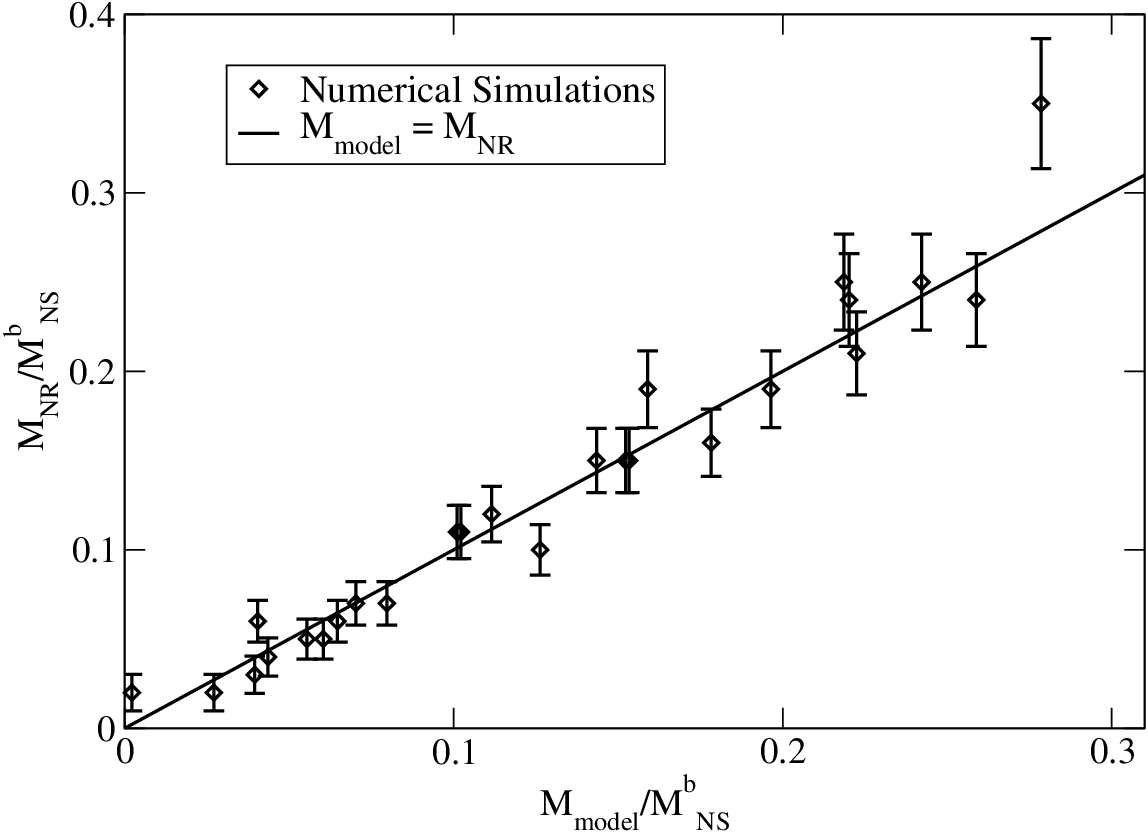
A comparison between the simple model and the numerical results is shown in Fig. 1, in which we plot as a function of for simulations 1-26. We can see that the difference between the modelled and measured masses is generally smaller than the errors expected from Eq. 11. The main exception is the large remnant mass observed in case 4. We suspect that our model, which assumes that the remnant mass scales linearly with and , breaks down for remnant masses greater than about of the neutron star mass. A non-linear relation between these distances and the remnant mass might perform better in that regime, but more numerical simulations are required to test that hypothesis.
V.3 Error Estimates
Estimating the error in the mass predictions of our model from the statistical errors in the parameters and is likely to be misleading. Differences between the numerical results and the predictions of the model come from multiple sources: the numerical error of course, but also a physical spread of the exact mass remnants around the predictions of the model. A part of that spread at least should be due to differences in the outcome of BHNS mergers for binaries with the same parameters (,,,), but different equations of state (i.e. neutron stars with the same radius but a different internal structure). This effect can also be seen in the differences between the predictions of models (6,9,10). But more generally, it is unlikely that the simple equations used here can perfectly represent the complex dynamics of a BHNS merger.
From the fact that we measured , we know that the errors are compatible with a gaussian distribution of variance . This is already indicative of the likely existence of a non-zero physical spread around the results of the model. The estimated numerical errors are indeed more of an upper-bound on the errors in the simulations than the width of an expected gaussian distribution. In the absence of a difference between the real physical outcome of a merger and the output of the model, we would thus expect to be lower than 1. How much of the measured errors comes from numerical errors and how much from actual differences between the model and the physical reality is hard to determine, especially considering that the numerical errors are not well known. A more cautious approach to estimate the uncertainty in the model is thus to consider as a conservative upper bound on the variance of a gaussian error in the model itself.

Fig. 2 shows contours of for various neutron star compactness. The general features of this plot are not surprising: the formation of massive disks is known to be favored by low mass ratios, high black hole spins and large neutron stars. But our model allows for the determination of the region of parameter space in which a certain amount of matter will remain available at late times with fairly high accuracy: at least within the spread or, if we consider a measurement of as a way to determine the radius of a neutron star, within .
Another important issue is the validity of the model outside the parameter range currently covered by numerical relativity. It is indeed possible that larger errors will be found for more compact neutron stars () or larger mass ratios (). However, given that our model fits the numerical data over a fairly wide range of parameters, and is derived from the physics of tidal disruption, it is likely to give decent results over most of the astrophysically relevant parameter space — with the notable exception of configurations leading to very large remnant masses (i.e. for nearly-extremal black hole spins and low mass ratios), and probably of the asymptotic regime where scalings valid in the range might break down. The differences between models (6,9,10) outside of the fitting region can also provide a rough estimate of these errors.
VI Discussion
VI.1 Parameter Space Study
The models described in the previous sections can be used to easily approximate the region of parameter space in which disruption occurs, or in which a certain amount of mass will remain available at late times. Such predictions are particularly important when trying to determine which BHNS mergers are likely to lead to short gamma-ray bursts (SGRBs): only BHNS mergers ending with the formation of a massive accretion disk could power SGRBs. Disruption of the neutron star is also a prerequisite for the ejection of unbound material, and thus for any electromagnetic signal due to the radioactive decay of a neutron-rich ejecta. If the neutron star does not disrupt, the only observational signatures of BHNS mergers are their gravitational wave emissions, as well as potential electromagnetic or neutrino precursors (see e.g. Tsang et al. [44]).
The minimum remnant mass required to get SGRBs is currently unknown, and is likely to vary across the parameter space: the fraction of the remnant mass which, at any given time, is in a long-lived accretion disk around the black hole (as opposed to the tidal tail or unbound ejecta) is by no means a constant, nor are the physical characteristics of that disk. We know, for example, that at high mass ratios a larger fraction of the mass is initially in an extended tidal tail than for lower mass black holes [10]. Furthermore, other characteristics of the disk (temperature, thickness, baryon loading along the rotation axis of the black hole, magnetic fields) are important for the generation of a gamma-ray burst. And what the ideal conditions are depends on the physical process powering the burst (see Sec. II for more details). Nevertheless, is already a useful prediction, providing a good estimate of the amount of material available for post-merger evolution. Additionally, any configuration for which can be immediately rejected as a potential SGRB progenitor.
Predictions for the mass of neutron star material remaining outside the black hole at late times are detailed in Figs. 3-5, in which we plot contours of the remnant mass as a function of the mass ratio and black hole spin. Each figure correspond to a different neutron star compactness, covering the range of radii expected from the theoretical results of Hebeler et al. [38]. Experimental measurements of neutron star radii are still fairly difficult, but studies of bursting X-ray binaries by Ozel et al. [45, 46, 47] tend to favor the lower range of potential radii ( km). Steiner et al. [39], after reassessing the errors in the measurement of neutron star radii from X-ray bursts, derived a parametrized equation of state which takes into account both the astrophysical measurements and results from nuclear theory. They predict that km for . We can thus consider Fig. 3 and Fig. 5 as bounding the range of potential neutron star radii, while Fig. 4 is around the most likely neutron star size (for stars — heavier stars are expected to be more compact).
The strong dependence of the remnant mass in the radius of the star is particularly noteworthy. In the most likely astrophysical range of mass ratios (), remnant masses can be achieved for moderate black hole spins if we consider neutron stars with (), as in Fig. 3. But at the other end of the range of potential neutron star radii, for (), the much more restrictive condition applies(Fig. 5). For a neutron star in the range of compactness favored by Steiner et al. [39] (, or ), keeping of the neutron star material outside the black hole requires spins , an already fairly restrictive condition (Fig. 4).


This naturally implies that the rate of SGRBs produced as a result of BHNS mergers is very sensitive to the equation of state of nuclear matter, and in particular to the size of neutron stars. Determining that rate is unfortunately impossible without knowledge of the number of BHNS mergers, and of the distributions of black hole spins and mass ratios. Additionally, a large enough is only a necessary condition for a given BHNS binary to power a SGRB. Knowledge of the exact properties of the accretion disk (and of the exact physical process leading to short gamma-ray bursts) would be required to accurately determine which BHNS systems are SGRB progenitors. Nonetheless, the importance of the equation of state can be fairly easily understood by simply computing the area of the region above a certain contour of for various values of . Let us define as the critical spin above which and
| (20) |
Then, represents the fraction of binaries with mass remnants greater than assuming that the distributions of mass ratios and spins are uniform within the and range respectively. As we decrease the size of the neutron star from to , Table 2 shows that we go from about of the parameter space in which significant disks are possible to about ! This does not necessarily mean that SGRBs are impossible for — but certainly indicate that they would occur in a non-negligible fraction of BHNS mergers only if quasi-extremal spins are the norm.
| 0.135 | 0.46 | 0.30 | 0.16 |
|---|---|---|---|
| 0.155 | 0.29 | 0.17 | 0.07 |
| 0.180 | 0.16 | 0.08 | 0.02 |
| 0.220 | 0.05 | 0.01 | 0.00 |

Current population synthesis models estimate the peak of the distribution of black hole masses in BHNS systems to be around , or [16, 17]. Fig. 6 offers clearer information on the behavior of BHNS systems in that regime. We see that no disk can form for unless . That condition becomes if we require at least outside the black hole at late times. Results for BHNS binaries with higher black hole spins () should of course be considered with caution: indeed, no mergers of BHNS binaries have been published for or , and such simulations would be required to rigorously test the accuracy of these predictions in extreme regions of the parameter space. Nonetheless, our model indicates that quasi-extremal spins are at least a necessary condition for the formation of massive disks for and .
The minimum spin requirement for massive disk formation across the parameter space of BHNS binaries is shown in Fig. 7, in which the black hole spin needed to keep of the neutron star mass outside the black hole at late times is plotted. Figs. 6 and 7 both indicate the existence of an extended region of parameter space (, ) which is likely to be astrophysically relevant but remains numerically unexplored, and in which the outcome of BHNS mergers varies significantly.

VI.2 Comparison with previous models
The tidal disruption of a BHNS binary is a complex problem, to which various approximations have been proposed. In the limit of very large black hole masses, Fishbone [23] derived the separation at which equilibrium tides would cause the disruption of an incompressible, corotating neutron star, a work that was generalized to compressible flows and irrotational binaries by Wiggins & Lai [24]. Such models have a few significant limitations, which were discussed in more details by Miller [25]. The innermost stable circular orbit of the black hole is only an approximation to the minimum separation at which stable circular orbits exist for finite mass objects. Analytical approximations to the location of the last stable circular orbit can be obtained from the Post-Newtonian expansion (see e.g. Damour et al. [26]). These show that for equal mass objects the last stable circular orbit can be well outside of the ISCO obtained in the point particle limit. An alternative to the analytical method, which avoids the complications resulting from the use of the Post-Newtonian expansion close to merger, is to consider sequences of quasi-equilibrium configurations computed numerically. This is the approach taken by Taniguchi et al. [27] to determine whether a neutron star in a BHNS binary would disrupt before reaching the last stable circular orbit (in the case of non spinning black holes). The numerical results also indicate that the innermost stable orbit is outside of the ISCO of the isolated black hole, although not by as much as the Post-Newtonian results would indicate.
Miller [25] also points out that the condition used in [26, 27] is only valid in the limit of infinitely slow inspiral. If the system looses angular momentum through the emission of gravitational waves, the plunge will actually begin outside of the last stable circular orbit, thus limiting further the ability of BHNS binaries to disrupt and form accretion disks. Additionaly, models based on equilibrium tides neglect the fact that, close to disruption, the rapid inspiral can cause the neutron star to be well out of equilibrium.
An alternative method is to simply fit a semi-analytical models to the result of numerical relativity, effectively attempting to include the complex physics that is not taken into account by the model into the free parameters of the fit. This is the approach taken by Pannarale et al. [28], in their model describing the neutron star as a tri-axial ellipsoid distorted by the tidal field of the black hole. That model was however fitted to general relativistic simulations at low mass ratio which have since been shown to have underestimated in many cases the mass of the remnant. At high mass ratio, no general relativistic simulations were available at the time, and the model was thus fitted to simulations using an approximate treatment of gravity, known to overestimate the ability of BHNS binaries to form disks. Our model takes a similar approach, fitting a rather simple physical model to more recent numerical data covering a wider range of binary parameters.
Compared to the predictions of Pannarale et al. [28], the results presented here indicate that it is a lot more difficult to create massive accretion disks at high mass ratios than what that previous model indicated, while at low mass ratios our model predicts significantly higher final masses. As opposed to [28], our model is unlikely to capture the behavior of BHNS mergers with , when finite-size effects begin to make it more difficult to form massive disks. These differences are expected considering what we now know of the limitations of the numerical data used to fit their model.
We can also revisit the condition derived by Taniguchi et al. [27] for the parameters allowing disk formation in the case of non-spinning black holes, and by Wiggins & Lai [24] for extreme mass ratios. Requiring is equivalent to imposing an upper bound on the neutron star compactness,
| (21) |
We find that our results are less favorable to tidal disruption and disk formation than in [27], as could be expected from the arguments of Miller [25] discussed at the beginning of this section. The predictions of Eq. (21) are on the other hand in agreement with the numerical simulations performed by Kyutoku et al. [12], even though the results for low mass ratio, non-spinning BHNS mergers published in [12] were not taken into account when fitting our model. In the high mass ratio limit, they also agree fairly well with the results of Wiggins & Lai [24] (within for ). This is however more of a test of the ability of our model to extrapolate to extreme mass ratios, well outside of the fitting region, than of the accuracy of the results of Wiggins & Lai, which are more reliable in that regime.
VII Conclusions
We constructed a simple model predicting the amount of matter remaining outside the black hole about after a BHNS merger, based on comparisons between the binary separation at which the neutron star is expected to be disrupted by tidal forces from the black hole and the radius of the innermost stable circular orbit around the hole. We show that the model can reproduce the results of recent general relativistic simulations of non-precessing, low-eccentricity BHNS mergers within a few percents of the total mass of the neutron star. The simplest best-fit model is
(in units in which ).
These mass predictions should be valid at the very least within the range of parameters currently covered by numerical simulations (, km, ), and are likely to remain fairly accurate within most of the astrophysically relevant parameter space. Alternative models using different approximations for the binary separation at which tidal disruption occurs are presented in Sec. III.
Using this model, it becomes easy to estimate the region of parameter space in which large amounts of matter remain outside the black hole for long periods of time. This is of particular importance when studying whether BHNS mergers can result in short gamma-ray bursts. Our results show the strong dependence of the remnant mass in the radius of the neutron star: whether the equation of state of neutron stars is at the soft or stiff end of its potential range could easily translate into an order of magnitude difference in the rate of gamma-ray bursts originating from BHNS mergers. It is also quite clear that high black hole spins are likely to be a prerequisite for the formation of massive disks. Neutron stars in the middle of the theoretically allowed range of radii () require spins for about 10% of the neutron star material to remain outside the hole, while quasi-extremal spins are necessary for the most compact stars.
The validity of our model is currently limited to black hole spins aligned with the orbital angular momentum and remnants below of the neutron star mass, due to the lack of numerical data available for precessing binaries and high mass remnants. Extending the model to cover these interesting parts of the parameter space would certainly be useful, but would require a large number of computationally intensive simulations to be performed (particularly to cover misaligned black hole spins). A few additional simulations using high mass ratios or small neutron star radii together with relatively large spins () would also be extremely helpful, allowing better estimates of the errors in the model for binary parameters which are astrophysically relevant but have never been considered by numerical relativists.
The extreme simplicity of these models should make them useful tools to obtain cheap but reliable estimates of the results of BHNS mergers across most of the astrophysically relevant parameter space, as well as to help determining which numerical simulations to perform in order to study given physical effects. This simplicity is, however, also a reason for caution: to accurately predict which BHNS systems would lead to the production of short gamma-ray bursts, modeling more physical properties will certainly be required: temperature, division of the mass between disk and tidal tail, neutrino emission, and magnetic field configuration are all important characteristics of the final remnant, as are the final properties of the black hole recently modeled by Pannarale [48]. More detailed models, however, might require a larger number of numerical simulations as the number of fitted parameters and the complexity of the problem increases. Finally, an improved understanding of the physical process leading to a burst will also be necessary before we can explicitly determine which BHNS binaries produce short gamma-ray bursts.
Acknowledgements.
The author thanks Harald Pfeiffer, Saul Teukolsky, Dong Lai, Christian Ott and Matthew Duez for useful discussions and suggestions concerning this project, and all members of the SXS collaboration for regular discussions and input. The author also wish to thank the participants of the ’Rattle and Shine’ conference at the Kavli Institute for Theoretical Physics for stimulating discussions on this topic. This research was supported in part by the National Science Foundation under Grant No.NSF PHY11-25915.References
- [1] ligo Scientific Collaboration, http://www.ligo.caltech.edu.
- [2] ego-virgo Scientific Collaboration, http://www.ego-gw.it.
- [3] J. Abadie et al., Classical and Quantum Gravity 27, 173001 (2010), eprint 1003.2480.
- [4] K. Somiya, Classical and Quantum Gravity 29, 124007 (2012), eprint 1111.7185.
- [5] W. H. Lee and E. Ramirez-Ruiz, New Journal of Physics 9, 17 (2007), eprint arXiv:astro-ph/0701874.
- [6] L. F. Roberts, D. Kasen, W. H. Lee, and E. Ramirez-Ruiz, Astroph.J.Letters 736, L21 (2011), eprint 1104.5504.
- [7] B. D. Metzger and E. Berger, Astroph.J. 746, 48 (2012), eprint 1108.6056.
- [8] K. Kyutoku, H. Okawa, M. Shibata, and K. Taniguchi, Phys. Rev. D 84, 064018 (2011).
- [9] Z. B. Etienne, Y. T. Liu, S. L. Shapiro, and T. W. Baumgarte, Phys. Rev. D79, 044024 (2009).
- [10] F. Foucart, M. D. Duez, L. E. Kidder, M. A. Scheel, B. Szilagyi, and S. A. Teukolsky, Phys. Rev. D 85, 044015 (2012), eprint 1111.1677.
- [11] F. Foucart, M. D. Duez, L. E. Kidder, and S. A. Teukolsky, Phys.Rev.D 83, 024005 (2011), eprint 1007.4203.
- [12] K. Kyutoku, M. Shibata, and K. Taniguchi, Phys.Rev.D 82, 044049 (2010), eprint 1008.1460.
- [13] M. D. Duez, F. Foucart, L. E. Kidder, C. D. Ott, and S. A. Teukolsky, Classical and Quantum Gravity 27, 114106 (2010), eprint 0912.3528.
- [14] M. D. Duez, Classical and Quantum Gravity 27, 114002 (2010), eprint 0912.3529.
- [15] M. Shibata and K. Taniguchi, Living Reviews in Relativity 14, 6 (2011).
- [16] K. Belczynski, R. E. Taam, E. Rantsiou, and M. van der Sluys, Astrophys. J. 682, 474 (2008), eprint arXiv:astro-ph/0703131.
- [17] K. Belczynski, M. Dominik, T. Bulik, R. O’Shaughnessy, C. Fryer, and D. E. Holz, Astroph.J.Letters 715, L138 (2010), eprint 1004.0386.
- [18] Z. B. Etienne, Y. T. Liu, V. Paschalidis, and S. L. Shapiro, Phys. Rev. D 85, 064029 (2012a), eprint 1112.0568.
- [19] S. Chawla, M. Anderson, M. Besselman, L. Lehner, S. L. Liebling, P. M. Motl, and D. Neilsen, Physical Review Letters 105, 111101 (2010), eprint 1006.2839.
- [20] Z. B. Etienne, V. Paschalidis, and S. L. Shapiro, ArXiv e-prints (2012b), eprint 1209.1632.
- [21] K. Kiuchi, Y. Sekiguchi, K. Kyutoku, and M. Shibata, Classical and Quantum Gravity 29, 124003 (2012), eprint 1206.0509.
- [22] W. H. Lee, E. Ramirez-Ruiz, and D. Page, Astrophys. J. 632, 421 (2005), eprint astro-ph/0506121.
- [23] L. G. Fishbone, Astrophys. J. 185, 43 (1973).
- [24] P. Wiggins and D. Lai, Astrophys. J. 532, 530 (2000), eprint arXiv:astro-ph/9907365.
- [25] M. C. Miller, Astrophys. J. Lett. 626, L41 (2005), eprint arXiv:astro-ph/0505094.
- [26] T. Damour, P. Jaranowski, and G. Schäfer, Phys. Rev. D 62, 084011 (2000), eprint arXiv:gr-qc/0005034.
- [27] K. Taniguchi, T. W. Baumgarte, J. A. Faber, and S. L. Shapiro, Phys. Rev. D 77, 044003 (2008), eprint 0710.5169.
- [28] F. Pannarale, A. Tonita, and L. Rezzolla, Astrophys. J. 727, 95 (2011), eprint 1007.4160.
- [29] R. Mochkovitch, M. Hernanz, J. Isern, and X. Martin, Nature 361, 236 (1993).
- [30] W. H. Lee, E. Ramirez-Ruiz, and J. Granot, Astrophys. J. Lett. 630, L165 (2005), eprint arXiv:astro-ph/0506104.
- [31] R. D. Blandford and R. L. Znajek, MNRAS 179, 433 (1977).
- [32] J. M. Bardeen, W. H. Press, and S. A. Teukolsky, Astrophys. J. 178, 347 (1972).
- [33] D. Lai, F. A. Rasio, and S. L. Shapiro, Astrophys. J. Suppl. 88, 205 (1993).
- [34] É. É. Flanagan and T. Hinderer, Phys. Rev. D 77, 021502 (2008), eprint 0709.1915.
- [35] T. Hinderer, B. D. Lackey, R. N. Lang, and J. S. Read, Phys. Rev. D 81, 123016 (2010), eprint 0911.3535.
- [36] T. Hinderer, Astroph.J 677, 1216 (2008), eprint 0711.2420.
- [37] B. D. Lackey, K. Kyutoku, M. Shibata, P. R. Brady, and J. L. Friedman, Phys. Rev. D 85, 044061 (2012), eprint 1109.3402.
- [38] K. Hebeler, J. M. Lattimer, C. J. Pethick, and A. Schwenk, Physical Review Letters 105, 161102 (2010), eprint 1007.1746.
- [39] A. W. Steiner, J. M. Lattimer, and E. F. Brown, Astroph.J. 722, 33 (2010), eprint 1005.0811.
- [40] N. Stone, A. Loeb, and E. Berger, ArXiv e-prints (2012), eprint 1209.4097.
- [41] B. C. Stephens, W. E. East, and F. Pretorius, Astroph. J. Letters 737, L5+ (2011), eprint 1105.3175.
- [42] W. E. East, F. Pretorius, and B. C. Stephens, Phys. Rev. D 85, 124009 (2012), eprint 1111.3055.
- [43] W. H. Press, S. A. Teukolsky, W. T. Vetterling, and B. P. Flannery, Numerical Recipes: The Art of Scientific Computing (Cambridge University Press, 2007), 3rd ed.
- [44] D. Tsang, J. S. Read, T. Hinderer, A. L. Piro, and R. Bondarescu, Physical Review Letters 108, 011102 (2012), eprint 1110.0467.
- [45] F. Özel, T. Güver, and D. Psaltis, Astrophys. J. 693, 1775 (2009), eprint 0810.1521.
- [46] T. Güver, P. Wroblewski, L. Camarota, and F. Özel, Astrophys. J. 719, 1807 (2010), eprint 1002.3825.
- [47] F. Özel, A. Gould, and T. Güver, Astrophys. J. 748, 5 (2012), eprint 1104.5027.
- [48] F. Pannarale, ArXiv e-prints (2012), eprint 1208.5869.