Searching for Stringy Topologies in the Cosmic Microwave Background

We assume the basic setup of slow-roll inflation in which the inflaton is a scalar field $\phi$. Then the orbifold identification (1) implies

where $\eta$ is conformal time. Quantum mechanically this means that

where $u(\eta,\mathbf{x})=a(\eta)\phi(\eta,\mathbf{x})$ (here $a(\eta)$ is the scale factor) and $\pi(\eta,\mathbf{x})$ is the canonically conjugate variable.

This yields the following commutation relation for the creation and annihilation operators

(and $[a_{\mathbf{k}},a_{\mathbf{k}^{\prime}}]=[a_{\mathbf{k}}^{\dagger},a_{\mathbf{k}^{\prime}}^{\dagger}]=0$). The second term is due to the orbifold point and, as expected, it breaks both homogeneity and isotropy.

Using these commutation relations we find that the theory is still Gaussian. Namely, only the two point functions do not vanish and yield

where $P_{\phi}(k)$ is the standard inflaton power spectrum, $H^{2}/2k^{3},$ evaluated at horizon crossing. Hence for the metric perturbation, $\Phi$, we get

where $P_{\Phi}(k)$ is the standard power spectrum. Note that violation of translational invariance was considered already in [15]. The approach taken in [15] is that this violation is small and the two point function can be expanded around the translational invariant term. In our case the contributions of the two terms in (6) are of equal magnitudes, and therefore we cannot use such an expansion, but rather use the exact form.

We made two hidden assumptions in deriving (6). First, we assumed that the string scale is much smaller than the Hubble scale during inflation. Otherwise, the stringy modes that are confined to the orbifold point will affect the inflaton power spectrum that is fixed at the Hubble scale. Second, we assumed that the compactifaction scale is smaller than the Hubble distance during inflation. The reason we are forced to make this assumption is that the orbifold point breaks SUSY and as such, leads to instabilities. To avoid this issue we can consider an orbifold that acts also on the compactified directions (that must exist in string theory) and that on large scales acts like (1). The simplest example is an orbifold point on $\mathbb{R}^{3}\times\text{S}^{1}$. If the radius of the $\text{S}^{1}$ is larger than the Hubble scale during inflation then (6) is a good approximation. These assumptions are often made and do not constrain the generality of (6) too much.

Equipped with eq. (6) the calculation of the harmonic coefficients of the temperature anisotropy is straightforward (though cumbersome) since the $a_{\ell m}$’s are determined by $\Phi_{\mathbf{k}}$ in the following way

Here $\Delta_{\ell}(k)\equiv\Delta_{T\ell}^{(S)}(k,\eta_{*})$ is the (scalar) response function and $\eta_{*}$ is the radius of the last scattering surface (LSS). In using the response function we are utilizing the “line-of-sight” approach [16], which takes into account the Sachs-Wolfe (SW) effect, the integrated SW effect on large scales and the Boltzmann physics of the coupled photon-baryon fluid on small scales.

We use (6) to calculate the covariance matrix of the harmonic coefficients

where

is the standard diagonal $\Lambda$CDM angular power spectrum and

is the departure of the correlation function from $\Lambda$CDM due to an orbifold located at $\mathbf{x}_{0}=r_{0}\hat{\mathbf{n}}$. In order to evaluate (10) we use the familiar expansion of an exponent in spherical harmonics

where $j_{\ell}(x)$ is the spherical Bessel function. We fix the coordinate system so that $\hat{\mathbf{n}}$ points in the $\hat{\mathbf{z}}$ direction, and get

where the matrix $A_{\ell m\ell^{\prime}m^{\prime}}$ is given by

The Gaunt integral $\mathcal{G}$ is defined by

and calculated using Wigner’s 3-$j$ symbols. It is non-zero only if $\ell_{1}+\ell_{2}+\ell_{3}$ is even, $m_{1}+m_{2}+m_{3}=0$ and $|\ell_{i}-\ell_{j}|\leq\ell_{k}\leq\ell_{i}+\ell_{j}$. Therefore, the matrix $A_{\ell m\ell^{\prime}m^{\prime}}$ is given by

The resulting correlation matrix is real, proportional to $\delta_{mm^{\prime}}$ and symmetric with respect to both $m\leftrightarrow-m$ and $\ell\leftrightarrow\ell^{\prime}$.

As a consistency check of this equation we take $r_{0}=0$. Then statistical isotropy is restored and the presence of the orbifold point implies that $C_{\ell}=0$ for all odd $\ell$’s. Indeed, since $j_{\ell^{\prime\prime}}(0)=\delta_{\ell^{\prime\prime}0}$, we get

which immediately gives the diagonal correlation matrix

as expected.

As we have seen, the sole effect of the orbifold point is the deformation of the covariance matrix of the harmonic coefficients without inducing non-Gaussianities. Schematically, we got $\mathbf{C}_{\text{orb}}=\mathbf{C}^{(0)}+\Delta\mathbf{C}$, where $\mathbf{C}^{(0)}$ is the standard $\Lambda$CDM covariance matrix. Since $\mathbf{C}^{(0)}$ is diagonal (when disregarding instrumental effects), the S/N for detecting the orbifold is [17, 18, 19]

Much of the signal is at high-$\ell$ where this calculation is extremely computationally intensive. Hence we use the expression expanded to leading order in $\Delta\mathbf{C}$,

where

The resulting expression depends only on the distance $r_{0}$ to the orbifold point.

In Fig. 2 we plot the S/N for each multipole $\ell$ and for a few values of $r_{0}$.

We see that as expected the S/N is a decreasing function of $r_{0}$. This is also apparent from Fig. 2, where the accumulated S/N up to $\ell_{\max}=200$ is shown.¹¹ 1 This scale corresponds to the $1^{\circ}$ resolution of the ILC map. We can see that the S/N drops fast as the orbifold location approaches the last scattering surface. Once outside, it can no longer be detected. On the other hand, as long as the orbifold is within the observable universe, $\text{S}/\text{N}>5$. There are two contributions to the ideal S/N, one on large scales ($\ell\lesssim 10$) and the other on intermediate scales ($\ell\sim 200$). The dominant intermediate scales contribution is due to the SMaC and its typical scale is fixed by the thickness of the LSS. In a more realistic setup, the finite beam size is expected to lower the S/N of small scales. We expect, however, that on intermediate scales the effect would be small since the beam size $\lesssim 1^{\circ}$. In addition the scanning strategy of WMAP is expected to have a direction dependent effect on the S/N, which for a general direction is also expected to be small.

Ideally, we would use the correlation matrix to search for an orbifold signature in the CMB data. In comparing the observed correlations with those of the model, we would utilize as much of the available information as possible. However, we now see that this approach is not feasible, as most of the signal lies in small scales, requiring the analysis of large matrices containing high-$\ell$ data. Since the orbifold model is not isotropic, such an analysis includes the generation of a large correlation matrix for each orbifold distance $r_{0}$ as well as its rotation to all orientations with respect to the data. We therefore have to search for an orbifold signature in a way that will not use all the available signal, but will be computationally feasible. This is done in the next subsection by focusing on the SMaC only.

As explained in the introduction, if the orbifold point is within the visible universe, we expect to find a SMaC in the CMB. The opening angle $\alpha$ of the circle satisfies

where $r_{*}$ is the radius of the LSS, as illustrated in Fig. 1. Every point on this circle is identified with another point on the circle, with a phase of $\pi$ separating the two. Therefore, the CMB temperatures of the two points match. If the CMB temperature fluctuations were comprised of the SW signal alone, we would see an exact image of the surface of last scattering and the match would be perfect. There are, however, other effects that add noise to this match. Experience from the celebrated search for matching circles [6, 7, 9, 11, 12], relevant for classical topologies, suggests that overall the S/N should be quite high if the circle is large enough. That is, the S/N for detecting the orbifold is expected to decreases with $r_{0}$. A larger $r_{0}$ means a smaller circle, and a smaller circle is harder to detect with high statistical significance.

The score for detecting a SMaC is the following. Compare each circle in the data with itself, rotated by a phase of $\pi$. We therefore consider, for each pixel $p$ and for each opening angle $\alpha$, the score

where $T_{p}(\alpha,\phi)$ is the temperature at phase $\phi$ along the circle centered at $p$ and the angle brackets denote integration over $\phi$. We follow [7, 9, 11, 12] and Fourier transform the temperature profile along the circle as $T_{p}(\alpha,\phi)=\sum_{m}T_{p,m}(\alpha)\exp(im\phi)$. We give appropriate weights to the different angular scales [9] and get

This score equals unity for a perfect match and for a random circle its expectation value vanishes.

In order to test if the CMB data contain a SMaC, we should examine all pixels $p$ and all angular radii $\alpha$. We use the HEALPix scheme [20] to search all directions using a grid with $N_{\text{side}}=256$, corresponding to a resolution of $\sim 0.25^{\circ}$. Following [7], when collecting data points along each circle, we linearly interpolate values at $2N_{\text{side}}$ points. For each $\alpha$, we record $S_{\max}(\alpha)$, the highest value of $S_{p}(\alpha)$ maximized over all pixels $p$. We search all angles in the range $20^{\circ}\leq\alpha\leq 90^{\circ}$ with a resolution of $0.25^{\circ}$.

We wish to verify that our score works as it should. To do that, we simulate CMB temperature fluctuation maps for a universe with an orbifold using the covariance matrix, calculated in §II.2. First, we get the response function $\Delta_{T\ell}^{(S)}(k,\eta_{*})$ from CMBFAST [16] using CMBEASY [21], a computation independent of the location of the orbifold. Then, we compute the covariance matrix $\mathbf{C}(r_{0})$ of an orbifold located in the $\hat{\mathbf{z}}$ direction. We perform a Cholesky decomposition of the positive-definite matrix to get the triangular matrix $\mathbf{L}$ satisfying $\mathbf{C}=\mathbf{LL}^{\dagger}$. We then draw a vector $x_{\ell m}$ of uncorrelated complex random Gaussian numbers of zero mean and unit variance, and compute the $a_{\ell m}$ coefficients as $\mathbf{a}=\mathbf{Lx}$. For an orbifold in a different direction, the coefficients can be rotated using a Wigner rotation matrix. Finally, the temperature fluctuation is given by $T(\hat{\mathbf{n}})=\sum_{\ell m}a_{\ell m}Y_{\ell m}(\hat{\mathbf{n}})$. We use $\ell_{\max}=200$ in our simulations. We plot $S_{\max}(\alpha)$ for a simulation with $r_{0}=0.5r_{*}$ in Fig. 3. We find that, as expected, there is a single spike, at the correct opening angle.

We can use simulated sky maps to determine the maximal distance to an orbifold that could still be detected with our SMaC score, namely the detection threshold. An orbifold located farther away cannot be detected with our score as its signal is obscured by the statistical noise of $\Lambda$CDM.

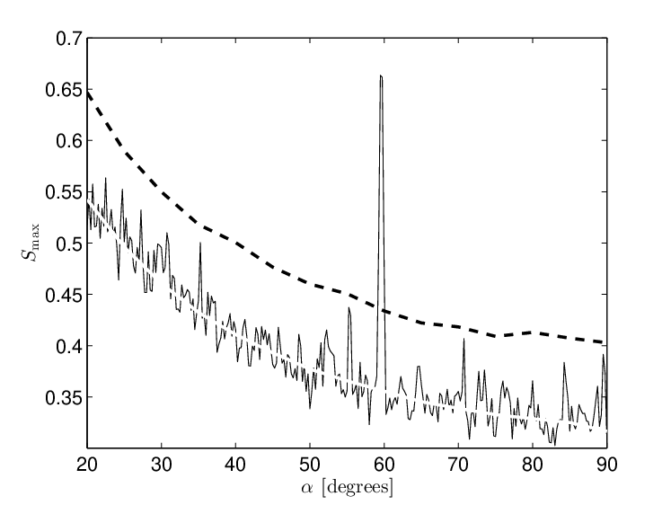
To estimate the noise, we simulate $\Lambda$CDM sky maps and calculate $S_{\max}(\alpha)$ for each of them and for each $\alpha$. We then define a false detection level (FDL) corresponding to a level of $3\sigma$ above the median of the score of the random $\Lambda$CDM sky maps.²² 2 Since $S_{\max}(\alpha)$ is not normally distributed we cannot use the mean and standard deviation of the distribution. We therefore use the median and the percentile corresponding to $3\sigma$ instead. This is the dashed line shown in Figs. 3, 4 and 5. It is important to note that the $3\sigma$ FDL we take has the meaning of local significance. By local, we mean the significance of a peak in $S_{\text{max}}(\alpha)$ with respect to that specific opening angle $\alpha$, and all directions. Of course, once a local peak is found, one needs to take into account the so called “look elsewhere” effect to estimate its true significance with respect to all radii and all directions. However, a peak with local significance lower than the FDL should not even be considered as a candidate for further analysis.

We plot $S_{\max}(\alpha)$ for a few values of $r_{0}$ in Fig. 4.

We can see that an orbifold which is located nearer to us (a SMaC with a larger radius) produces a higher spike in $S_{\max}(\alpha)$, and is therefore easier to detect. In addition, an orbifold located at a distance of $r_{0}=0.85r_{*}$ does not produce a peak in $S_{\text{max}}(\alpha)$ that is significant enough to cross the FDL, setting the detection threshold to $\sim 0.85r_{*}$.

The above analysis holds for a clean sky. A more realistic scenario, however, must take into account foreground contamination. Even when working with the ILC map, we should still be cautious about pixels that lie inside the galactic mask, as they can affect the matching circle and change the score. For instance, if an orbifold resided in the direction of the galactic north pole at a distance corresponding to, say, $\alpha\sim 80^{\circ}$, its SMaC would lie entirely inside the mask, risking undetectability even though according to Fig. 4 an orbifold at such a location should be easily detected. The mask can also affect smaller circles, with an arbitrary portion of the circle inside the mask.

Since the mask is anisotropic, the FDL is also direction dependent. This in turn means that the detection threshold is direction dependent as well. We demonstrate this by considering two directions that have recently been found to be related to CMB anomalies and examining the dependence of the score on the orientation with respect to the mask. The first is $(l_{1},b_{1})=(266^{\circ},-19^{\circ})$, normal to the reflection plane exhibiting large scale odd parity [22, 23], and the second is $(l_{2},b_{2})=(276^{\circ},-1^{\circ})$, around which [24] found giant concentric rings. In order to generate a simulation with the galactic plane contaminated, we rotate an orbifold simulation so that the orbifold point is in the relevant direction, and replace the data inside the KQ75 galactic mask with those of a random $\Lambda$CDM realization. While this procedure for contaminating the galactic plane obviously does not realistically model any residual galactic foregrounds, it is merely used here to demonstrate the orientation dependence of such effects. After contaminating the same orbifold simulation in orientations suitable for directions $\hat{\mathbf{n}}_{1}$ and $\hat{\mathbf{n}}_{2}$, we search for the SMaC with our score. The results, for $r_{0}=0.3r_{*}$ as an example, are plotted in Fig. 4, where it is clear that the orientation affects the level of contamination. Varying $r_{0}$ and repeating this analysis, we find the detection threshold for these directions. We get $0.35r_{*}$ and $0.4r_{*}$ for $\hat{\mathbf{n}}_{1}$ and $\hat{\mathbf{n}}_{2}$, respectively, a significant change from the clean-sky isotropic $0.85r_{*}$.

Unfortunately, calculating an orientation-dependent FDL is not feasible. Therefore, we are left with our isotropic FDL and the naive estimate for the detection threshold. If the data of WMAP show any peaks in $S_{\max}(\alpha)$ that cross the FDL, we should check each candidate and see whether its orientation with respect to the mask is such that it could be heavily contaminated. On the other hand, there is also a chance that a SMaC does exist in the CMB and it is too contaminated for us to detect.