Non-diagonal charged lepton mass matrix and non-zero $\theta_{13}$

From all the possible three-zero textures (shown in Eq. (III)) only the following provide (real) solutions: $M_{304}$, $M_{308}$, $M_{309}$, $M_{310}$, $M_{311}$, $M_{312}$, $M_{313}$, $M_{314}$, $M_{315}$, and $M_{316}$.

For the textures $M_{301}$, $M_{302}$, $M_{303}$, $M_{305}$, $M_{306}$, and $M_{307}$ we did not find any solution. The reason is that all these textures lead to an extra constriction because the matrix product $M_{l}M_{l}^{T}$ has a zero entry. Those entries are $(M_{301}M_{301}^{T})_{12}$, $(M_{302}M_{302}^{T})_{13}$, $(M_{303}M_{303}^{T})_{12}$, $(M_{305}M_{305}^{T})_{13}$, $(M_{306}M_{306}^{T})_{23}$, and $(M_{307}M_{307}^{T})_{23}$.

As mentioned above, once we have performed all calculations (including the normalization of the mass matrix by the VEV of the Higgs field) we find the maximum and minimum orders of magnitude of the entries for each texture of the Yukawa matrix. They are shown here (up to $O(1)$ coefficients):

As part of the analysis we performed, we searched for the solution volume of each three-zero texture, that is, the set of points given by the three mixing angles that make possible to find real solutions to the entries of the $M_{l}$ matrix.

In the case of textures $M_{308}$ – $M_{316}$ the solution volume fills the complete space given by the experimental intervals of the three mixing angles (the experimentally allowed parameter space). This happens for both $\delta=0$ and $\delta=\pi$.

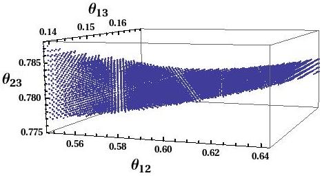
The most interesting case is the texture $M_{304}$, which has the zeros on the major diagonal (and its permutations). The relevance of this case is that the angle $\theta_{23}$ is now very restricted. Thus, we took a closer look within a smaller interval for $\theta_{23}$ using a finer grid of $40\times 40\times 40$, and analyzing a $\theta_{23}$ interval of $[0.7745,0.7950]$, we find that the solution volume of $M_{304}$, for both $\delta=0$ and $\delta=\pi$, is a thin curved surface (presented in Figure 1 for $\delta=\pi$); the only difference between these two cases is a displacement of the interval allowed for $\theta_{23}$, which is $[0.7763,0.7876]$ for $\delta=0$, and $[0.7750,0.7873]$ for $\delta=\pi$. These intervals are near but exclude the central value of $\theta_{23}$.

The Yukawa matrices in (68) can explicitly be written as

Then, the diagonal entries $(Y_{l}Y^{T}_{l})_{ii}$ are just the sum of the square of the elements of the i-th row of $Y_{l}$:

The textures obtained in Subsection IV.1 present some interesting features: first note that in all textures the largest upper bound ($10^{-2}$) always appears in the second row. Thus, from Eq. (70), $(Y_{l}Y_{l}^{T})_{22}\sim O(10^{-4})$. This is a little higher than $O(m_{\tau}^{2}/{\langle H\rangle}^{2}\sim 5\times 10^{-5}$). Note also that (except for the $Y_{304}$) the third row has always an upper bound of $10^{-3}$ and then, from Eq. (70), we can deduce that $(Y_{l}Y_{l}^{T})_{33}\sim O(10^{-6})$. This is quite close to the value of the ratio $m_{\mu}^{2}/{\langle H\rangle}^{2}\sim 10^{-7}$. More precisely and using the explicit values of the Yukawa matrix of Eq. (67) we find

We thus find that there are extra conditions on the entries of $Y_{l}$ in terms of the charged leptons masses. Because of equation (5), we can expect that these conditions may be due to an internal structure of the mixing matrix $U_{l}$ for the charged leptons. In what follows we show that there is indeed a parametrization for this matrix that leads to specific relations between the entries in the Yukawa matrices and the charged lepton masses that reproduce the above results, including the small deviations in the orders of magnitude.

Motivated by the fact that the charged leptons are analogous to the down type quarks in terms of representations of the Standard Model gauge group, we consider a CKM-like parametrization for the $U_{l}$ mixing matrix in terms of the three angles $\theta_{12}^{l}$, $\theta_{13}^{l}$ and $\theta_{23}^{l}$, taking values between $0$ and $\pi/2$, and all phases set to zero in order to use real values for the $U_{l}$ matrix, as we have done in the whole analysis. Then, we can write:

Using $U^{\prime}$ instead of $U_{PMNS}$ (to avoid agglomeration of indexes) one can easily find that:

Here the $\theta_{ij}$ are, as before, the parameters of $U_{PMNS}$; different from $\theta_{ij}^{l}$, which parametrize $U_{l}$. We evaluated equations (73)-(75) with $\theta^{l}_{ij}\in[0,\pi/2]$, and took all the points that matched the experimental intervals given by (62) and (63). The points ($\theta^{l}_{23},\theta^{l}_{13},\theta^{l}_{12}$) are presented in Figure 2.

In Figure 2 the blue region is made of those values of the angles that solve equation (73) within the experimental values, the purple points are those that solve equation (73) and (74) within the experimental ranges, and the dark yellow region is the set of points that satisfies the three equations (73), (74) and (75) within all the experimental values. We then obtain a small region given by two small angles and a large one:

Now we use the parametrization of the $U_{l}$ matrix given by equation (72) and the values of its angles to make an analysis of the entries in a general charged lepton mass matrix, of the form given by (6). Let us remember that $U_{l}$ appears in (5). Using the values given in (76), one can built a simpler form for $U_{l}$. Indeed, according to equation (72) and using the fact that $\theta^{l}_{12}$ and $\theta^{l}_{13}$ are small, we can use a first-order approximation for their respective rotation matrices. The size of the angle $\theta^{l}_{23}$ allows us to use a first order approximation too, but around $\theta^{l}_{23}=\pi/2$. Then, $\sin(\theta^{l}_{23})\approx 1$ and $\cos(\theta^{l}_{23})\approx\frac{\pi}{2}-\theta^{l}_{23}\equiv\epsilon$. Thus, we end up with:

Using (77) in (5), we obtain the matrix $M^{2}_{l}$ in terms of $\theta_{12}^{l}$, $\theta_{13}^{l}$ and $\epsilon$. Comparing the result with (7), we can see that the variables from the first row of the mass matrix must satisfy:

the variables of the second row of (6) satisfy:

and the third row of (6) must have a contribution of the form

These expressions explain the observations considered at the beginning of the present subsection, including the corrections to the order of magnitude estimates, and represent the main result of this analysis.

Taking our specific example above, dividing equations (78)-(80) by $\langle H\rangle^{2}$ as in (68), and using the values $\theta_{12}^{l}=0.09$, $\theta_{13}^{l}=0.1215$, $\theta_{23}^{l}=1.55$ as well as the central values for the charged lepton masses we have:

These are the values from (71), which are relations that exhibit the dependence of the entries of $Y_{l}$ on the masses and the mixing angles of $U_{l}$. It is easily observed that for the first row, although the leading term (zeroth order on the angles) is $m_{e}^{2}$, the other contributions play a more important role than this one, because the masses of the $\mu$ and $\tau$ leptons are much greater than that of the electron and even overcome the small size of their coefficients (which are powers of the angles). Finally, we note that these expressions are independent of the texture chosen for the Yukawa matrix and also independent of the two values of the Dirac phase used in the PMNS matrix.

All the Yukawa textures found exhibit the relations given by equations (78)-(80), so an important feature that we want to point out is that the matrices we have found show a very large mixing (nearly $\pi/2$) between the second and third generations of the charged leptons.

We have already explored the textures with three zeros and found that it is possible to have solutions in the allowed ranges for many of them. Now we are interested in checking if this is also possible for textures with four zeros. To start, we list the possible textures with four zeros and their equivalent (column) permutations, discarding those with a row or column completely filled with zeros (thus avoiding singular matrices):

We have also calculated the product $M_{l}M_{l}^{T}$ for each texture and we can observe that most of them render one or two zero entries. As in the previous case, this increases the difficulty in finding solutions to the system of equations in Eq. (5). Moreover, since we are assuming only real values in the mass matrix entries, for the four-zero textures we are left with $6$ equations and only $5$ variables to satisfy them and the system is over-constrained.

The zero entries in the product $M_{l}M_{l}^{T}$ for each texture are the following:

The only textures which give non-zero entries in $M_{l}M_{l}^{T}$ are $M_{411},M_{415},M_{416}$, and $M_{417}$. Those would be the more interesting cases to study if we allow complex parameters (this would imply also to allow the $\delta$ CP violating phase to take all its possible values). $M_{412}$, $M_{416}$ and $M_{418}$ also render non-zero entries in $M_{l}M_{l}^{{\dagger}}$ but they are singular.

We performed a scan over all the allowed experimental range for the mixing angles trying to solve the system of equations for each particular texture, in the case of real parameters, without success. The only possibility is to consider cases where one of the zero entries in the four-zero texture gets slightly turned on. This case could correspond then to one of the three-zero texture above where one of the entries is much smaller than all others. Analyzing the three-zero textures and the relative size of their entries (presented above), we observe that except for $M_{304}$, all of them contain entries in the range $(10^{-4}-10^{-3})$ – $10^{2}$ MeV, and that the smallest one is at least two orders of magnitude smaller than the next one. It is then possible, from a model building perspective, to consider a four-zero texture where one of the zeros is lifted (perhaps due to radiative corrections, or higher order operator mixings) such that at the end one ends up with one of the successful three-zero textures above. Here we show which four-zero texture could be used in such a scenario

As a final remark we comment that even though at this point we considered only real matrices for the charged lepton mass matrices, it is possible to extend some of our results to the case of complex matrices with factorizable phases, i.e. mass matrices that can be written as $M_{l}=P^{*}\hat{M}_{l}P$, where $\hat{M}_{l}$ are matrices with real entries and $P$ a diagonal phase matrix, $P=\text{diag}(e^{\imath\phi 1},e^{\imath\phi 2},e^{\imath\phi 3})$ . Then, if $\mathcal{O}_{l}$ is the orthogonal matrix which diagonalizes $\hat{M}_{l}\hat{M}_{l}^{T}$ we can write, under our assumption $U_{\nu}=U_{TBM}$, $\mathcal{O}_{l}=P^{*}U_{TBM}U_{PMNS}^{T}$. Nevertheless, from the property of orthogonality and $\det\mathcal{O}_{l}=\pm 1$ we can infer that the only possible values for the factorizable phases are integer multiples of $\pi$. We checked exactly the same three-zero textures as before, but allowing complex entries and a CP-violating phase $\delta=\pi/2$ and found solutions for the same textures as in the real case. The difference with our previous results is that in these cases solutions are found in all the allowed volume of angles, even for $Y_{304}$, and the order of magnitude of the entries are generally larger. In the four-zero texture we again find no solutions and due to the fact that the entries in the three-zero textures are larger in this case, it is not possible to easily start from a four-zero texture and lift one zero (here we are thinking of a naturally small correction to the zero entry in question).