Bulk-edge correspondence for two-dimensional topological insulators
Abstract
Topological insulators can be characterized alternatively in terms of bulk or edge properties. We prove the equivalence between the two descriptions for two-dimensional solids in the single-particle picture. We give a new formulation of the -invariant, which allows for a bulk index not relying on a (two-dimensional) Brillouin zone. When available though, that index is shown to agree with known formulations. The method also applies to integer quantum Hall systems. We discuss a further variant of the correspondence, based on scattering theory.
1 Introduction
Topological insulators are materials that behave as ordinary insulators in the bulk, in that they exhibit an excitation gap, whereas the edge has robust, gapless modes. They have been theoretically predicted as a class [16] and as a specific compound [2], in which the effect was then observed [19, 15]. In analogy with quantum Hall (QH) systems, the presence of edge states is a robust property of the system, in that it is stable under moderate changes of parameters. That calls for an explanation in terms of topological invariants.
As pointed out in [16], a key feature of topological insulators is fermionic time-reversal symmetry. It was shown that two-dimensional time-reversal symmetric insulators admit two topologically distinct phases: The phases can not be deformed into one another as long as the bulk gap and the symmetry are there. In one phase the insulator is an ordinary one; that is, it does not carry currents in the bulk nor at the edges. In the other phase edge states are present. They come in pairs with opposite velocity and spin. This phase is called the quantum spin Hall (QSH) phase and its signature is a nonzero spin current, which in contrast to the QH current is not quantized, as a rule. For integer quantum Hall systems the topological invariant is a Chern number, and can be read off from the value of the Hall conductivity; for quantum spin Hall systems the topological invariant is not expressing the value of the spin current, but the parity of the number of edge states.
In this paper we prove the bulk-edge correspondence for two-dimensional topological insulators and for independent particles. For short we introduce a bulk topological invariant (to be shown equivalent to others), and we show that it is equal to the number of pairs of edge states modulo . For sure, that duality has been discussed in the literature, see e.g. [9], but we maintain that there is room for a strict mathematical approach; just as for quantum Hall systems, where Laughlin’s argument has gained in precision and detail by the subsequent mathematical discussion. We should though mention [25, 1], whose results are further compared to ours below.
The paper is organized as follows. In Section 2.1 we consider a general class of two-dimensional single-particle lattice Hamiltonians, with and without edge. They are symmetric under fermionic time reversal and hence potentially describe topological insulators. One noteworthy feature is that periodicity is postulated only in the direction parallel to the edge. In Section 2.2 we formulate the duality in its most basic version, in a precise though still preliminary form. The purpose of Section 3 is to show how graphene and related model materials, which have been considered as candidates for topological insulators, fit into our scheme. As a side remark, we give a simple new proof of the absence of edge states for armchair boundary conditions. In Section 4 we discuss some abstract vector bundles on the 2-torus. By considering their sections and transition matrices, we classify them in terms of a -invariant, defined similarly but not identically to one found in [9]. So equipped, we define the bulk index in Section 5 and state in full the basic version of duality (Theorem 5.4). It is immediately followed by the main steps of the proof, while technical details are postponed to main part of Section 7. The part of the article so far described provides a full and self-contained account of basic bulk-edge duality. It is the most general part, and yet makes up for less than half of its length.
In Section 5.1 we formulate a bulk index for the specific and more familiar case where the lattice Hamiltonian is doubly periodic. As it is to be expected, the relevant 2-torus is now the Brillouin zone. We discuss how that index arises from the general one, leaving details to Section 8. All the results obtained up to that point have a counterpart in the case of QH systems, which we present in Section 6 for illustration, because they are simpler in that context. As a matter of fact, for such systems we include an independent, alternate version of the duality based on scattering theory and more precisely on Levinson’s theorem (Section 6.2), as well as a comparison between the two versions (Section 6.3). Related details are found in Section 9. We conjecture an analogous alternate version for QSH systems. Finally, Section 7.1 contains some results about indices, including a comparison of ours with some of those found in the literature.
Let us comment on the relation to other work. In [16] an edge and a bulk characterization of a topological insulator is given, but without proof of a mathematical link. In [25] a correspondence between bulk and edge description is given. There however the bulk is put in correspondence with twisted boundary conditions allowing tunneling between a pair of edges; they include open boundaries as a special case. Moreover, the bulk invariant used there is physically different from a -classification and may not reflect itself in open boundaries. In [1] the bulk-edge duality for topological insulators is derived in the same sense as ours, among other results. The setting, however, is not quite as general as ours, as far as the side of the bulk is concerned. As the edge is concerned, an index related to the Maslov index is defined and shown to be equivalent to that of [16]. As for the bulk, it is assumed that the Hamiltonian is the perturbation of one commuting with spin, and hence consisting to several copies of a quantum Hall system. It is assumed that the gap remains open as the perturbation is switched on. Thus spin resolved Chern numbers can be defined by homotopy [24, 29] and the duality inferred from that of the quantum Hall case [28].
Further, assorted comments are: Some of our examples are discussed in [1] in a similar vein. Related indices for topological insulators are discussed in [1, 9, 12, 16, 20, 27]. A bulk-edge duality result for general symmetry classes is found in [4], differing from the results presented here in various ways; for instance the index takes values in , with just hints at the case, at least in two dimensions. A choice of a torus and bundle similar to ours in Sect. 2.2 is found in [30]. The results of Section 5.1 depend on the analytic properties of band functions [18]. In [13] bulk-edge duality for Hall systems is pinpointed at the birth of edge states of band edges. This insight is the reason for using Levinson’s theorem, though the method is otherwise different and the result more general. Last but not least, the existence of a complementary approach to gapped systems, including interacting ones, should be mentioned. It is based on effective, topological field theories as a tool to explore the response of a system in the limit of low frequencies and long wavelengths; see [31, 5, 8, 32, 6, 7] for early examples.
2 Setting and results
We shall introduce a class of bulk, resp. edge, single-particle discrete Schrödinger operators, by which we describe insulators, topological or otherwise, which extend over a plane, resp. a half-plane. We conclude the section with a loose description of the results.
2.1 The Schrödinger operators
Consider, at first and in less than final generality, a tight binding Hamiltonian with nearest neighbor hopping on the lattice , resp. . The Hamiltonian is assumed to be periodic in the direction along the edge, but not necessarily across it. The period may be taken to be equal to one without loss: In fact sites within a period may be regarded as labels of internal degrees of freedom, among others like e.g. spin. We may thus perform a Bloch decomposition with respect to the longitudinal quasi-momentum , which remains a good quantum number even in presence of the boundary.
We so end up with a family of Hamiltonians defined on the one-dimensional lattice , resp. , and acting on wave-functions , where is the number of internal degrees of freedom.
More generally, these objects are stated as follows.
Definition 2.1.
[Bulk Hamiltonian] The Hamiltonian, acting on and parametrized by , is
| (1) |
The potential and the hopping matrices are matrices having a -dependence on , uniformly in . We assume , where ∗ denotes the matrix-adjoint, and that . (Recall that consists of invertible matrices of order .)
We then consider the restriction of the Hamiltonian to (we find it convenient to omit zero), while allowing for changes within a finite distance from the edge.
Definition 2.2.
[Edge Hamiltonian] The Hamiltonian, acting on , is
| (2) |
where satisfies the above properties of , as well as
| (3) |
Moreover we assume the Dirichlet boundary condition, meaning that for Eq. (2) is to be read with .
Remark 2.3.
The Dirichlet condition is by no means special. Since
any boundary condition , () defines a self-adjoint Hamiltonian if . That amounts to the Dirichlet condition after adding to .
Contrary to what the above motivation might suggest, the Hamiltonians (1, 2) are prompted by more than just the square lattice. In the next section we will show that several models based on the honeycomb lattice, which have been considered [16] in relation with the quantum spin Hall effect, fit the scheme. Moreover, one-dimensional spin pumps [9] also match the description, with playing the role of time.
The topological classification applies to insulators that are invariant under odd (or fermionic) time-reversal symmetry. In the sequel we specify these notions.
Definition 2.4.
[Time-reversal symmetry] The symmetry is a map with the following properties.
- i)
is antilinear and ;
- ii)
;
- iii)
For all ,
(4) where also denotes the map induced on . Likewise for .
As a result, is even. In the models described in the next section, properties (i, ii) arise from the time-reversal of a spin- particle, and (iii) from the symmetry of the Hamiltonian.
The Bulk Hamiltonian of an insulator is supposed to have a spectral gap at Fermi energy and for all :
| (5) |
Typically does not satisfy the gap condition. In fact, while for the essential spectra we have , the edge Hamiltonian may have discrete eigenvalues crossing for some values of .
2.2 The main result in brief
We can informally introduce two indices, , defined in terms of and , respectively. On the circle the involution has two fixed points, . The edge index is the parity of the number of those at which an eigenvalue of equals , at least if the eigenvalue crossings are simple. The index requires more explanation. By definition does not have eigenvalues ; yet we may regard the Schrödinger equation
as a second-order difference equation in . As such, it has linearly independent solutions, but we focus attention on those which decay as . They form a linear space, , of dimension . By (i, iii) we have
and thus . We choose a reflection symmetric complex contour, , encircling the part of the spectrum of lying below , and we set . We so have: (a) an involution on the torus ; (b) a vector bundle with base and fibers ; which (c) are compatible with in the stated sense. To any vector bundle with these features, including (i), but irrespective of the concrete definition of its fibers, an index will be associated in Sect. 4. The bulk index is that index for the particular bundle arising from as described. The main result of this work is that .
It should be noted that the result relies on just one translational symmetry.
3 Examples
We show how to obtain Hamiltonians (1, 2) from the Schrödinger operator on the honeycomb lattice, which models graphene in the single-particle approximation. We will consider two types of boundary conditions: zigzag and armchair. It is known that the spectrum of the Schrödinger operator depends on which boundary condition is chosen, [21, 14]. In particular, a zigzag boundary implies the presence of zero-energy edge states, while they are absent for the armchair boundary. In Example 3.1 we give a new proof of the last statement.
3.1 Graphene
Let be the (infinite) honeycomb lattice and its bipartite decomposition into two triangular lattices , . Upon fixing an origin, they are
Any site in has three nearest neighbors in , shifted by or by another equivalent vector. See Fig. 2. The model for graphene is simply the Schrödinger operator for a particle hopping between nearest neighbors (with hopping parameter ).
The (Bravais) lattice of translations of is . We reduce to by dimerizing neighbors shifted by . We retain the position of the -site as that of the dimer, and the values of the wave function at the two sites as pseudospin components:
| (6) |
With these notations, the Schrödinger operator takes the form
| (7) |
The expression for could of course have ended up differently. Let us name the choices underlying its construction: a sublattice shift vector (above: ), defining the dimer, and two primitive lattice vectors ( and ), defining adjacency between dimers. For instance for , , and hence , , Eq. (7) becomes
after dropping primes. See Fig. 3.
The Bloch decomposition w.r.t.
| (8) |
fibers the Hamiltonian, . In fact we obtain from Eq. (7)
where we set , and
| (9) |
Likewise for :
| (10) |
where now
It should be noted that only the second Hamiltonian satisfies the condition in Eq. (1). The two equivalent bulk Hamiltonians no longer are once they are turned into edge Hamiltonians by means of the Dirichlet boundary condition. Indeed, they correspond to (a) zigzag and (b) armchair boundary conditions, respectively. See again Fig. 3.
Proposition 3.1.
(i) The Hamiltonian has as an eigenvalue. Actually, has it for . (ii) The Hamiltonian does not have any eigenvalue, i.e. its spectrum is purely continuous.
Proof. i) Related to being singular, reduces to the first order equations
The boundary condition implies , but is ineffective for , for which there is a non-trivial solution in , as long as , i.e. for in the stated range.
ii) Every second dimer of the armchair boundary is exposed (see Fig. 3 right) and the axis containing them is . Let us consider, on the whole lattice , the reflection of lattice sites about the axis in Fig. 3, as well as parity, . Clearly, . Any odd eigenfunction of satisfies the Dirichlet boundary condition on the line , whence its restriction to defines one for . What matters more is that the converse is true as well: The odd extension of satisfies the Schrödinger equation on , and hence at all . The conclusion is by noting that has no eigenvalues; actually it has purely absolutely continuous spectrum. This is known and by the way has a short proof: It suffices to establish the property for the fiber Hamiltonian . Since the latter has real analytic Bloch eigenvalues , absolute continuity holds unless is constant in . That, finally, is ruled out by in Eq. (10) and the remark below.
Remark 3.2.
([1], Prop. 7) Suppose the Hamiltonian on
(note: independent of ) has a Bloch eigenvalue independent of the quasi-momentum . Then is singular.
Proof. Let be that eigenvalue. Then for , () and, by analyticity, for . Letting gives . .
3.2 The Kane-Mele model
In the next example we discuss a model with odd time-reversal symmetry. Wave functions are now of the form , where labels dimers, see Fig. 2, and . The spin of the particle is represented by the Pauli matrices , , acting on the second factor . The time-reversal operator is , where denotes complex conjugation, which is the usual expression for a spin- particle.
Let be the Schrödinger operator on the honeycomb lattice defined in Eq. (7). We consider the operator
where the last term implements a spin-orbit coupling. There describes hopping between next-to-nearest neighbors; it thus acts diagonally on the pseudospin components of Eq. (6), and specifically as
| (11) |
with
The grouping of terms reflects that, starting from a given -site, its next-to-nearest neighbors are reached by turning right or left at a -site. The turns go along with phases modeling a magnetic flux through any (positively oriented) triangle ; yet the total flux through the hexagonal cell vanishes, since no phases are associated with the bonds forming its boundary, see Eq. (7). Likewise for and interchanged, resulting in the sign in (11). Indeed, for a given dimer, the next-to-nearest neighbors form again dimers, but the turns linking , resp. -sites are opposite.
The model is the special case of the Kane-Mele model, [16], where two further terms (a Rashba term and a staggered chemical potential) have been set to zero. Even so, it exhibits a non-trivial topological phase, i.e. , for small and . In fact, it is the direct sum of (a special case of) the Haldane model [11], , and of its time-reversed copy . In such a situation we have , where is the integer associated with the quantum Hall effect of . In the stated regime, a band gap of order opens, and , [11].
4 Time-reversal invariant bundles
The purpose of this section is to define the index of bundles of the kind mentioned in Sect. 2.2, see Def. 4.8 below, as well as some auxiliary indices; and to formulate some of their properties. We refer the reader to Sect. 7 for the proofs of the lemmas stated here.
4.1 The index of endpoint degenerate families
We shall define an index for certain families of points on the unit circle. We will give the most general definition, in order to make evident the stability of the index under homotopy. At the end of this section we give a procedure to compute it in a more restrictive setting, which is suitable for our application.
Following ([17], Sect. II.5.2) we consider unordered -tuples of complex numbers . A distance is defined by
where the minimum is taken over all possible relabellings of or . Let us recall ([17], Thm. II.5.2): Given a family , , which is continuous w.r.t. , there exists a (non-unique) continuous labeling .
In the following we will consider -tuples with . Any continuous labeling induces continuous arguments , i.e. . Two simple observations are in order: (i) is independent of the choice of arguments, as well as of labeling. In fact is independent of the latter. (ii) Any family with has a winding number given as
| (12) |
We next consider endpoint degenerate families : for each occurs with even multiplicity. We may concatenate such a family with one, , , such that and , while keeping even degenerate. Clearly, is not unique, but by (12)
By the same reason, is an integer; by it is determined by .
Definition 4.1.
[Index] We set
| (13) |
as the index of endpoint degenerate families.
Consider now the special situation where there is such that occurs only at finitely many , which moreover are simple crossings: for a single , and . Then
| (14) |
where is the number of crossings of . Indeed, one can choose without crossings of . Then is the number of signed crossings of by but that qualification is irrelevant for parity.
4.2 The index of Kramers families of matrices
Let be the matrix of even order given by the block diagonal matrix with blocks
the complex conjugation, and the standard time-reversal on . Suppose satisfies
| (15) |
Then the eigenvalues of come in pairs , with equal algebraic multiplicity, which is moreover even if . In particular their phases are even degenerate regardless. Indeed, , as seen inductively for ; for the corresponding pairs of eigenvectors remain linearly independent by .
Definition 4.2.
[Kramers property] We call Eq. (15) the Kramers property. We say a family , which is continuous in , has that property if the endpoints and have it.
The repeated eigenvalues of form a continuous family in the sense of the previous section ([17], Thm. II.5.1), and so do the . Moreover, is an endpoint degenerate family.
Definition 4.3.
All it in fact takes for the definition is the endpoint degeneracy of and not the stronger Kramers property of . However we shall not need such an extension.
Lemma 4.4.
Suppose
with continuous (), as well as
| (17) |
Then has the Kramers property, and has it iff does. If so,
| (18) |
The claims are of immediate verification, except for Eq. (18). However in the special case that the equality
| (19) |
is also immediate, because , then have the same eigenvalues. That case suffices for the basic result on bulk-edge duality.
4.3 The index of time-reversal invariant bundles
Let be the circle and the torus with involution . It has four fixed points: . Let be a complex vector bundle with base and fibers of dimension . We say that is time-reversal invariant if there is a map with and antilinear.
We also consider the associated frame bundle with the following operations induced on frames :
- •
right multiplication by :
(20) with . Any two frames are so related by a unique .
- •
, , with . Note that
(21)
In order to classify time-reversal invariant bundles we consider the torus cut along the circle , or more precisely . Note that only remain among the fixed points of , and that any bundle on naturally defines one on .
Lemma 4.5.
[Existence of time-reversal invariant sections] On the cut torus , there are (smooth) sections of the frame bundle (whence ) satisfying
| (22) |
As a result, they are compatible with right multiplication by iff
| (23) |
We remark that the condition (22) was shown [9] to be obstructed on the (uncut) torus by the -invariant.
Let be the boundary values of along the two sides of the cut, and the transition matrix,
| (24) |
Lemma 4.6.
[Time-reversal symmetry of the transition functions]
In particular, has the Kramers property on the interval , which hints at a the possibility of assigning an index to the bundle.
Lemma 4.7.
[Independence of the index from the section] Let , () be time-reversal invariant sections on the cut torus , and let the corresponding transitions matrices across the cut. Then
We may thus proceed to the following definition.
Definition 4.8.
Such bundles can hence be distinguished in two topologically distinct classes, according to the value of the index.
We also retain the following remark, which appears as a byproduct of Lemma 4.5.
Remark 4.9.
Let satisfy the time-reversal symmetry condition (i) of Def. 2.4. Then there is a basis of such that . If condition (ii) applies too, the basis can be chosen orthonormal. Letting map to the standard basis of , a restatement is with unitary.
5 The bulk-edge correspondence
It pays to look at first at wave-functions as just sequences, i.e. . It can be shown that for any in the resolvent set, the Schrödinger equation has linearly independent solutions which are square-integrable at . Let the linear space they form. As explained in Sect. 2.2 we obtain a vector bundle
| (26) |
over the torus , which enjoys the property of being time-reversal invariant. The following definition is thus natural.
Definition 5.1.
The edge index has been loosely introduced in Sect. 2.2. In preparation for precise definition let us take a closed interval containing the Fermi energy in its interior and such that for . The spectrum of is discrete and finite in (uniformly in ), and the eigenvalues are locally given by branches which are in ([17], Thm. II.6.8). By possibly adjusting we can arrange that if for some then . We note that the number of crossings at or is even by (4).
Definition 5.2.
Let be the number of crossings , with those at endpoints counted half. Set
as the edge index.
The next remark about the edge index is inessential for the following main result.
Remark 5.3.
The index could be also defined in terms of a Kramers family. To this end let be a continuous real function with , () and , (), where is the aforementioned interval. Then, in view of , the operator has the Kramers property, albeit w.r.t. , which is however irrelevant. The definition would be legitimate, since that of in Sect. 4.1 extends to countable families of points , as long as only finitely many (uniformly in ) are . It would agree with Def. 5.2 by Eq. (14).
Theorem 5.4.
We can give the main steps of the proof right away. For given we consider, besides of , also the linear space of solutions decaying at of the Schrödinger equation , without imposing boundary conditions at . Eq. (3) establishes a bijection
| (28) |
determined by for .
Frames consists of -tuples of linearly independent solutions . Note that the index does not denote the lattice site . Since , we may equivalently say: with belongs to iff is a solution of decaying at , which is moreover fundamental in the sense that for any
| (29) |
The bijection (28) induces one between frame bundles, , . It is manifestly compatible with the right action (23) of . The next lemma rests on the bijection.
Lemma 5.5.
- i)
A point has for some (and hence all) iff . If so, then . For a dense set of Hamiltonians near the given one, the points are isolated in and for each of them there is a simple eigenvalue branch with , ; moreover,
(30) Density is meant with respect to the topology of the class of Hamiltonians specified at the beginning of Sect. 2.1.
- ii)
Let be a section defined in a neighborhood in of any of the crossing points . The family of matrices
has the reflection property . Its eigenvalues are thus real for real . There generically is a single eigenvalue branch of vanishing to first order at : There the derivatives and are real and non-zero.
- iii)
At any of the points we have
(31) - iv)
As increases past the eigenvalue crosses as an increasing function if
and as a decreasing one in the opposite case.
The lemma, which is proven in Sect. 7, allows to complete the proof of the main result. As a matter of fact, only items (i, ii) matter to that end. For later use we mention that no use of time-reversal symmetry has been made in the lemma, in the sense that the statement about density of the Hamiltonians in (i) holds in either class, with and without that specification.
Proof of Thm. 5.4. As a preliminary we recall Remark 4.9: At the price of conjugating the Hamiltonians by in the internal space , which preserves the assumptions, we may assume
| (32) |
By density it will suffice to prove the theorem for Hamiltonians as specified in part (i) of the lemma. By the first sentence there, we can define a section away from crossing points by requiring
| (33) |
Clearly, the requirement can not be imposed at such points. In a small reflection symmetric disk containing the generic crossing point , Eq. (30) allows us to make an alternate choice by requiring
| (34) |
Based on the latter section we shall extend the former to the cut torus , where the cut is the Fermi line . On the boundary both sections are defined, and we have
| (35) |
for and some matrices , see Eq. (20), which are parametrized by in the interval resulting from the intersection of the Fermi line with . The same matrices relate and . We may then obtain the announced extension by (re)defining through Eq. (35) for . We observe that the section on so constructed satisfies Eq. (22); in fact its ingredients (33, 34) do by (32) and .
The transition matrix across the cut differs from the identity only within the intervals . Along such an interval the boundary values of the section are , resulting in the transition matrix
| (36) |
We can compute the bulk index using Eq. (14). The theorem then reduces to the claim that, for each crossing point, the eigenvalues of change with from 1 to 1 without winding, except for a single one with winding number .
It is with the proof of this claim that our choice of sections comes to fruition. In fact, by Eq. (33) and the sentence after Eq. (35) we have
We apply part (ii) of the lemma to the section , which is as required there. Then by Eq. (34) and hence
with for . Clearly, can be dropped, as it does not affect the eigenvalues under investigation. We have
where is the rank projection on the eigenspace corresponding to the eigenvalue , and is regular as a map on the range of the complementary projection. Clearly, as , but by (ii) above we also have on . We use the notation and for the value of a function and its gradient at the critical point. Then
In view of for we compute
| (37) | |||
In the second line we used , as seen from expanding . Using from , we find that is strictly block triangular. For small and the eigenvalues of (37) wind as if the error is omitted, provided those of the explicit part do not vanish. Those in turn remain the same when is omitted, and are in fact equal to with multiplicity , and to with multiplicity , where , (). The winding number of along equals that of along . Since the vanishing at the crossing point is of first order, , that number is
as claimed. Though the sign is irrelevant (so far), we observe that by (iv, v) it is if the eigenvalue crossing is decreasing in .
5.1 The bulk index as an index of Bloch bundles
A feature of definition of the Bulk index is that it applies to Hamiltonians which are periodic just along the edge, see Eqs. (1, 27). If the Hamiltonian is periodic in both directions and hence the Brillouin zone two-dimensional, the Bulk index allows for an alternate formulation in terms of the bundle of Bloch solutions, as we are about to explain.
We temporarily suppress the longitudinal quasi-momentum in Eq. (1) and consider Hamiltonians of of the form
| (38) |
where and is periodic in , i.e. . By once again considering sites within a period as labels of internal degrees of freedom, we may assume that the period is . This amounts to the replacement of , , by
| (39) |
In particular is singular, unlike . A Bloch solution of quasi-periodicity ,
| (40) |
and of energy is then represented as a solution of
| (41) |
For and , the matrix is hermitian, since now . It thus has eigenvalues (real and increasingly ordered) and eigenvectors , . The ranges of the energy curves are known as energy bands. Let
| (42) |
be the gap between successive bands of , where we temporarily reinstated the dependence on , implicit in (38). The gap is open if . Let then . In topological insulators the bands are degenerate for , in fact at . A band thus can not be separated from the rest of the spectrum, but a pair of them can. We will assume so for the pairs , , i.e.
| (43) |
where (even) is the uppermost band below the Fermi energy . For that band we actually retain the stronger assumption (5) of a spectral gap. (It amounts to a positive gap in Eq. (42) for even when extremizing jointly in , .)
Definition 5.6.
The Bloch bundle of the -th pair of bands has the Brillouin zone as base and the span as fibers.
It should be noted that while the eigenvectors are not smooth in , , their span is ([17], Sect. II.1.4), since degeneracies occur within the pair.
The result of this section is that the Bulk index can be expressed by means of the indices of the Bloch bundles of the filled pairs of bands.
Theorem 5.7.
Note the bundles seen on the two sides of Eq. (44) have different base spaces and fibers; in fact the dimensions of the latter are and , respectively.
The proof we will give makes the simplifying assumption that the energy curves do not have more critical points than required by the time-reversal symmetry of the Hamiltonian.
At first, we reduce the theorem to a lemma. The base space of the bundle in Eq. (26) can be extended from to all of . In this notation, . The torus may then be deformed and split into tori , each surrounding a pair of bands . Unlike , the do not need to be a Cartesian product form, since (43) does not imply a spectral gap uniformly in . We then consider the bundles . By homotopy and by the multiplicative property under splitting (Lemma 7.5), we have:
and Eq. (44) reduces to the following.
Lemma 5.8.
| (45) |
The proof of this main lemma is deferred to Sect. 8.
6 Quantum Hall systems
Much of what has been said in the previous sections has a counterpart for Hall systems. In that case the results are not completely new; nevertheless they generalize the bulk-edge correspondence of [13].
The setting is the same as given by the Hamiltonians (1, 2) with gap condition (5), but without postulating a time-reversal symmetry. For the sake of brevity, definitions and statements given in the sequel rely on notations and contexts used for topological insulators.
Definition 6.1.
Let be the vector bundle with base and fibers of dimension . On the frame bundle , the right multiplication by is defined as in (20).
The classification of such bundles may again proceed by considering the cut torus . In fact on there are smooth sections ; this is in analogy to Lemma 4.5, but with simpler proof, as observed in Remark 7.1.
Definition 6.2.
The index is just the Chern number of , but that will not be needed.
Definition 6.3.
Theorem 6.4.
Let bulk and edge index be defined as above. Then
Proof. The proof is contained in that of Thm. 5.4. Now its last sentence matters.
6.1 The bulk index as an index of Bloch bundles
We consider the case of doubly periodic Hamiltonians in close analogy to Sect. 5.1. As in Thm. 5.7 we will express the bulk index in terms of the Bloch bundles of the filled bands.
In the context of quantum Hall systems it is legitimate to assume that, for fixed longitudinal momentum , the bands do not overlap:
| (49) |
where is again the uppermost band below the Fermi surface, cf. (44).
Definition 6.5.
The Bloch bundle of the -th band has the Brillouin zone as base and the lines as fibers.
Theorem 6.6.
Proof. Consider the simplifying assumption that the energy curves do not have more critical points than necessary in absence of time-reversal symmetry, as explained after Eq. (50) below. The proof then parallels that of Thm. 5.7, but is much simpler. In fact the complex loop is of the type seen in the first case of Fig. 7, but run through just once.
6.2 Bulk-edge correspondence through scattering theory
We propose a further perspective on the bulk-edge correspondence in the doubly periodic case. It does not rely on decaying bulk solutions, as Thm. 6.4 did. In contrast to that result, where edge states are intercepted at Fermi energy, here they are right at inception, i.e. as they are born at band edges. That will be done by means of a result from scattering theory known as Levinson’s theorem. In its usual form ([26], Thm. XI.59) it computes the phase of the scattering matrix at thresholds. The version below computes the phase difference when a parameter is changed.
We focus on a single band which is separated from its neighbors,
| (50) |
and on its Bloch bundle , cf. Def. 6.5. We also assume that, for fixed , the energy curve has as a function of just two critical points, both non-degenerate, namely a maximum and a minimum (That assumption would not be consistent with topological insulators, cf. Fig. 7.) The curves cut the Brillouin zone into two open domains (resp. ) where is increasing (resp. decreasing) in w.r.t. the orientation of .
Lemma 6.7.
- i)
There is a map defined by and the property that is has the two extrema as its only fixed points. It interchanges and is real analytic in .
- ii)
There is a domain and on there a section of the Bloch bundle which is smooth in and analytic in .
We will occasionally omit from the notation in the sequel. In order to ensure that edge states are indeed “born at band edges”, we make the assumption that there are none embedded in the band,
| (51) |
The assumption is generically satisfied, but counterexamples can be constructed by taking the direct sum of two Hamiltonians, such that the pure point edge spectrum of one overlaps the band of the other.
Lemma 6.8.
At energies , the edge Hamiltonian has a bounded eigensolution which is unique up to multiples. It satisfies
| (52) |
where the Bloch solution is uniquely determined by . (We recall the relation (39) between and .) Hence is a section of on .
The bounded solution ought to be interpreted as a scattering solution for the reflection at the boundary . In fact, since on , represents an incoming wave, and an outgoing one.
Since and overlap near we may introduce scattering amplitudes for near and , resp. :
| (53) |
The scattering amplitudes , which by the lemma do not vanish, play the role of transition matrices (24) for the line bundle . Therefore, by (47),
where is defined in (46).
Definition 6.9.
We say that has a semi-bound state at the upper band edge if it admits a bounded solution of .
Lemma 6.10.
Suppose that a branch of discrete eigenvalues of touches the -th band from above at , i.e.
| (54) |
Then has a semi-bound state.
Theorem 6.11.
[Relative Levinson Theorem] Let , not correspond to semi-bound states of . Then
| (55) |
where denotes a continuous argument and is the signed number of discrete eigenvalue branches of emerging or disappearing at the upper band edge, as runs from to in the orientation of . Likewise for the lower band edge and , except for a reversed count of signs in .
In particular the theorem may be applied to , i.e. to a full circle . Then it states , . If is the uppermost band below the Fermi energy, then . If the same assumptions hold true for all bands below it, then the bulk-edge correspondence
is recovered in view of .
The proofs of the results of this section are found in Sect. 9.
6.3 Comparison between two approaches
In this section we compare the independent approaches to bulk-edge correspondence underlying Thms. 6.4 and 6.11.
Let have a semi-bound state at the isolated point . Suppose that a branch of discrete eigenvalues disappears there into the -th band from above, cf. Eq. (54) with , whereas none emerges; see Fig. 6. By a suitable, -dependent energy shift we may assume that the upper band edge is constant, and pick the Fermi energy arbitrarily close to it. The branch is then decreasing and crosses the (dashed) Fermi line. For , near with we have
for close enough to , where is the transition matrix (36) across the Fermi line, as used in the proof of Thms. 5.4 and 6.4. In fact, the first equation is the specialization of Eq. (55) and the second one follows from the claim made after Eq. (36). In case of an emerging branch the r.h.s. of both equations would change sign.
Both expressions on the l.h.s. arose as winding numbers. The point we wish to make here is that their equality can also be seen by homotopy, rather than by separate evaluation. We thus emphasize:
Proposition 6.12.
Under the above assumptions we have
| (56) |
The proof is given in Sect. 9.
We close this section with a remark. The duality of Sect. 6.2 relied on the assumption that, for fixed , the energy curve had a single local maximum and minimum in . That naturally assigns a unique outgoing wave to a given incoming one, with transversal momenta . Should the assumption fail, multiple reflected waves could arise, preventing that essential assignment; at least without further ado, like dealing with scattering matrices instead of amplitudes. That failure is in fact unavoidable for time-reversal symmetric Hamiltonians (see Fig. 7 left). However, Prop. 6.12 still indicates that the index of the Bloch bundle (associated to the pair of bands ) can be determined by the glitches of along the lines of global maxima (or minima). In fact points where edge state emerge or disappear generically occur only on those lines, see Eq. (51), whence at nearby energies scattering remains described by a single amplitude .
7 Basic bulk-edge correspondence: Proofs
The present section contains the proofs of our basic results for topological insulators (Thm. 5.4) and for integer quantum Hall systems (Thm. 6.4). We begin by supplying those relating to Sect. 4 (except for Lemma 4.4) and concerning the index of an abstract time-reversal invariant bundle.
Proof of Lemma 4.5. The main claim (22) states that there are linearly independent vectors such that
, i.e.
| (57) |
We first consider either fixed point . We will prove by induction in that there are linearly independent vectors , such that (57) holds true for . Indeed, pick such that are linearly independent and set . Then Eqs. (57) also hold for by . Moreover are still linearly independent: implies, by , the same with ; or for short for instead of . Since the rank of those vectors is at least we have
with , . Applying yields and together by .
The frames at the two fixed points may be interpolated over the line . In fact, there the bundle is trivial ([22], Cor. 9.5), since is contractible to a point; and is connected. Eq. (22) is then used as a definition to extend to a section over the circle .
The section may then be extended further to the half torus by homotopy. (We still denote by the bundle restricted to it.) More precisely, two maps are clearly homotopic, namely the identity map and . Hence and are equivalent bundles ([22], Thm. 9.4). Since the latter has fibers , the above section over the circle extends trivially to ; by equivalence the same holds true for . Finally, Eq. (22) extends the section to all of . An inspection of the procedure shows that the necessary smoothness of the section can be ensured. Eq. (23) then follows in the equivalent form using (21).
Remark 7.1.
In absence of time-reversal symmetry, see Sect. 6, the existence of a global section on is quite obvious. In view of the above we may just note that it exists on the circle . In fact we may pick any frame and interpolate along .
Proof of Lemma 4.6. Note that Eq. (22) states for the boundary values. We thus have
Since and the right action is transitive, the claim follows.
Proof of Lemma 4.7. The two sections obey the relation for some matrix continuous on . Let be its boundary values. The two transition matrices are then related by
| (58) |
More generally, we consider
as a homotopy in of families in . Eq. (23) implies that, at fixed , the matrices satisfy (17). Hence the family has the Kramers property. Clearly the index of is constant in by continuity. Note that one end of the homotopy is
which by (19) has the same index as , while the other is (58). We conclude .
We next come to the the proof of the main technical lemma in relation with the bulk-edge correspondence.
Consider the finite difference equation with and without imposing the boundary condition . Solutions are square-summable at iff for some . Hence is eigenvalue of iff is an eigenvalue of the operator , which now includes the boundary condition. In particular is then real, because is self-adjoint. For as in Fig. 1 we have .
We may arrange for the absence of “flat” crossings, , , by adding to and in Eqs. (1, 2) an arbitrarily small constant. In particular, the points are isolated, as claimed. Moreover, they are generically simple. To show this, we perturb , by and determine the splitting , of a degenerate eigenvalue of . On general grounds is found by diagonalizing after orthogonally projecting it onto the unperturbed eigenspace of . Here, that eigenspace is the image of under . Hence the eigenvalue problem reads
| (59) |
where is the orthogonal projection onto . By Eq. (29) the matrix in brackets on the r.h.s. is positive definite on , while that on the l.h.s. may take arbitrary Hermitian values, along with . As a result, the eigenvalues are generically distinct and, since , the points split into non-degenerate ones. Similarly, points with correspond to being a Dirichlet eigenvalue for . Its perturbative splitting is determined by (59) with the replacement of by . By (29), , so that the operator on the l.h.s. can be chosen with independent projections under and . Any coincidence between eigenvalues of the two Dirichlet problems is thus generically lifted.
The above argument did not pay attention to the time-reversal symmetry of the Hamiltonian and hence of . We do so now: A crossing at may be displaced by perturbing by an arbitrarily small constant; one at by letting satisfying Eq. (4). It still remains arbitrary at .
In preparation for the proof of part (ii) let us introduce the Casoratian, which is to finite difference equations what the Wronskian is to ordinary differential equations (both linear and of second order). Let be as in Eq. (38). Given , with viewed as column, resp. row vectors, let
| (60) |
Suppose that satisfy the Schrödinger equation in the form
| (61) |
where . Then
- C1)
is independent of and denoted .
- C2)
Let solve the first Eq. (61). Then solves the second. In particular is well-defined.
- C3)
Items (C1–2) apply if are replaced by .
Property (C1) follows from the identity
| (62) |
and Eq. (61); the others are straightforward. The Casoratian may be extended literally to matrix solutions of Eqs. (61), in which case is itself a matrix. Its entries are the Casoratians of the rows and columns of , resp. . Properties (C1–3) hold correspondingly.
Proof of Lemma 5.5, continued. ii) We drop and notice that
By (C2) the l.h.s. equals ; whence the reflection property. The statement about the eigenvalue branch follows from part (i) and the definition of .
iii) We drop . Let be the normalized eigenvector of with eigenvalue , whence by (30). Thus,
Next we observe that
because of (62) and of . Since , , we conclude . Actually, equality is excluded, because is positive definite, as remarked earlier.
iv) Let the eigenvalue branch crossing at , whence near . The claim follows from
together with (31).
7.1 Supplementary results
This section contains a few details related to Sect. 4, some of independent interest and some needed in connection with Thm. 5.7, but none with the proof of the basic results, which is by now complete. Also addressed is the relation with other indices found in the literature.
Polar decomposition. Given a matrix , let be its (unique, left) polar decomposition, i.e. , .
Lemma 7.2.
Let satisfy Eq. (15). Then so does and the following deformations of retaining that property are possible: (i) to , while keeping the polar part fixed; (ii) to , while preserving unitarity; (iii) and hence to .
Proof. The right polar decomposition is with . Eq. (15) states and is hence equivalent to
| (63) |
In particular the preliminary claim holds true.
i) Denoting by , () the spectral decomposition of , the second Eq. (63) is equivalent to the existence of an involution such that and . By interpolating the eigenvalues but not the eigenprojections, it becomes clear that can be deformed as stated.
ii) Denoting now by , () the spectral decomposition of , the first Eq. (63) is equivalent to . By again interpolating eigenvalues only we arrange for going to .
Let us also mention the following consequence:
Remark 7.3.
Let be the polar decomposition of . If the family has the Kramers property, then so does . Even though the are generally not the eigenvalues of , it holds true that .
Proof. By (i) of the previous lemma, can be continuously extended to the right on an interval in such a way that there Eq. (15) holds throughout, , and . Likewise on an interval . By continuity neither index, or , changes in the process. At this point they are manifestly equal. In fact is a convex set; hence any continuous map with is homotopic to .
Proof of Lemma 4.4. As mentioned, only Eq. (18) requires proof. Consider the families
They enjoy the Kramers property along with ; they can be concatenated, since ; and is homotopic to , as seen by postponing the change of till after that of . Hence
where by deforming to while preserving (17); and by Lemma 7.2 (iii).
Alternate definition. There is an alternative way to Def. 4.8 of computing the index of a time-reversal invariant bundle . Let be a section satisfying (22) on the twice cut torus , where exchanges the left and right halves of . The section gives rise to four boundary values and two transition matrices parametrized by :
| (64) |
Lemma 7.4.
In this situation, the families enjoy the Kramers property and
| (65) |
Def. 4.8 corresponds to the special case of a single cut at , whence ; a single cut at could have been used there instead.
Proof. The two families are Kramers because Lemma 4.6 still applies. Let be a time-reversal invariant section as in Lemma 4.5 and let , () be the change of frame . It satisfies (23). Since is continuous along and satisfies (24) along we have
where , . By Eq. (18),
As remarked in the proof of Lemma 4.7, the family is Kramers for fixed . It is continuous in in that interval, and its index constant. Hence the claim.
Splitting the torus. We consider a time-reversal invariant bundle on the torus , as described in Sect. 4.3. We suppose moreover that is a distinguished pair of lines in the sense that
| (66) |
(In applications, that identification of fibers may occur because the bundle is effectively the pull-back of another one under a map with .) Let us define the torus with identified edges , whence it still has four time-reversal invariant points. By (66) is a well-defined time-reversal invariant bundle. Similarly for and .
Lemma 7.5.
[Splitting lemma] In the situation set by Eq. (66) we have
| (67) |
Proof. By Lemma 4.5 there exists a section of satisfying (22) on , the torus cut along ; likewise, on with cut . Let , be the corresponding transition matrices (24). By (66) we may also introduce transition matrices , () by
| (68) |
Multiplying by , from the left, resp. right we obtain
and thus
| (69) |
Moreover, the l.h.s. of (68) is independent of , whence
| (70) |
On we define the section
It is continuous by (68) and satisfies (22): by hypothesis for , but also for by (69). Its transition matrix is read off as
Indices in the literature. The -index has been introduced in various other forms before [16, 9], but to our knowledge not in the form (25). We shall first recall a formulation [9] (there connected to [16]), which rests on an additional, metric structure, and later establish equivalence with ours when there is overlap. Like our index, it first deals with continuous families of matrices , () which, in lieu of the Kramers property, enjoy antisymmetry at endpoints . There,
where is the Pfaffian of ; in between, consider continuous branches . One of them will connect to , where defines the index of the family, cf. ([9], Eq. (3.24)). In the special case that , and hence , the index reduces to
| (71) |
where is the winding number of , ().
Let us move on to time-reversal invariant bundles . They are assumed equipped with a compatible hermitian metric, i.e. with an inner product on any fiber such that . Use is made of the fact that is trivial if is disregarded. There thus is a section of on the torus . We stress: not just on the cut torus , but at the price of forgoing time-reversal symmetry. It can be taken to consist of orthonormal frames . Let
see [12] and ([9], Eq. (3.16) with switched). Then and . By this last property, one may define the index as
where , , ; see ([12], Eq. (10)). The relation to the indices of the present work is as follows.
Proposition 7.6.
[Relation between indices]
- i)
Suppose , has the Kramers property and is antisymmetric at endpoints. Then
(72) - ii)
For a time-reversal invariant vector bundle as above we have
Proof. We begin with a preliminary remark. Consider the three properties of a matrix :
called Kramers, unitarity and antisymmetry, the first one being indeed a restatement of Eq. (15). In terms of they respectively read
Clearly any two of them imply the third.
i) The assumptions imply that are unitary. By Lemma 7.2 (ii) we may deform the family at its endpoints in such a way that , while retaining the Kramers property and unitarity, and hence antisymmetry. In the process both indices (72) remain defined and constant. At this point, see Eqs. (13, 16), , where is the winding number of . The claim follows by (71) and .
8 The bulk index as an index of Bloch bundles: Proofs
As a preliminary to the proof of Lemma 5.8, we consider Eq. (41) not just for , but for , together with its characteristic polynomial
| (73) |
Its basic properties, to be proven later, are as follows.
Lemma 8.1.
is a polynomial of degree in and a Laurent polynomial in of degrees and . Moreover
| (74) |
and, in the time-reversal invariant case , also
| (75) |
(As a function of that case holds true for .)
We then consider the Riemann surface (Bloch variety) defined by
| (76) |
where . We make some assumptions, which are typically true: is non-singular as a Riemann surface, meaning that at all points ; and, if either partial derivative vanishes, the corresponding second derivative does not. As a result, near a point where we can solve as with analytic; and if at a critical point , then , but . Similarly for interchanged roles of variables and at branch points. We conclude that eigenvalue branches have only non-degenerate critical points, and only branch points of order 2.
For we will have to exceptionally allow singular points where both derivatives of vanish. However they shall be ordinary double points, i.e. the Hessian of is non-degenerate.
Of importance is also the real Bloch variety
| (77) |
In fact, for any let be the number of with and , i.e. of points . Then implies , since now and becomes the characteristic polynomial of a hermitian matrix. Moreover is the multiplicity of as a point of the spectrum . By (74) the remaining points with come in pairs , . In particular is even.
For each we consider the (geometric) eigenspace of the eigenvalue of the matrix seen in Eq. (73).
Lemma 8.2.
For
is a line bundle with base and fibers .
In order to properly state the relation between this bundle and we make the following definition.
Definition 8.3.
A generalized Bloch solution of energy and quasi-periodicity satisfies and
| (78) |
where is a Bloch solution for the same .
Eq. (78) characterizes a generalized eigenvector (of order 2) of the translation operator. In terms of Eq. (39) a generalized Bloch solution corresponds to with
Lemma 8.4.
Let the eigenvalue branch have a critical point at and let be a local section of at . Then corresponds to a generalized Bloch solution for .
Finally, we consider
equipped with the projection
| (80) |
The preimage of a point consists of points iff . In that case we have
where the l.h.s. is to be understood as a direct image: The fiber at is with sum over ; the equation itself on rests on the relation (39) between and . Some care applies at points where , i.e. to a multiple (in fact, double) preimage of , because this seemingly results in a missing solution on the l.h.s.. It should however be read so as to include the there existing generalized Bloch solution. Equivalently, for near the fiber is of dimension and has a limit (of the same dimension) as . With this reading both sides are continuous in .
Likewise, the preimage of a loop is a cycle in , possibly consisting of several loops, and we have
| (81) |
Besides of we consider the projection
and the bundle . Its fibers are of dimension , even at branch points by continuous interpretation.
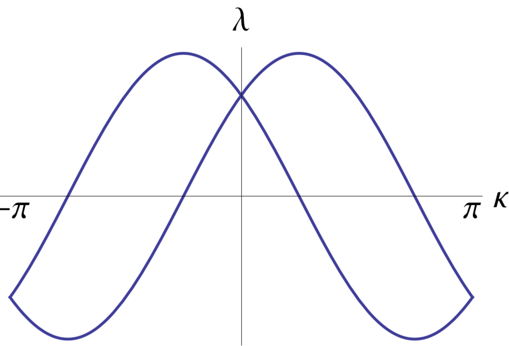
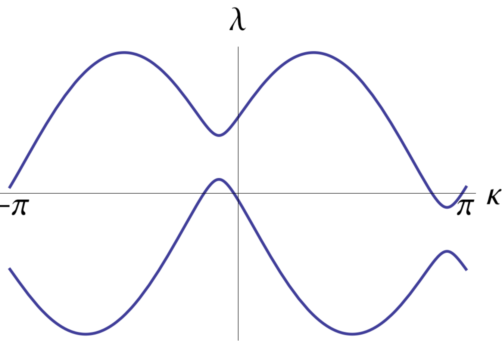
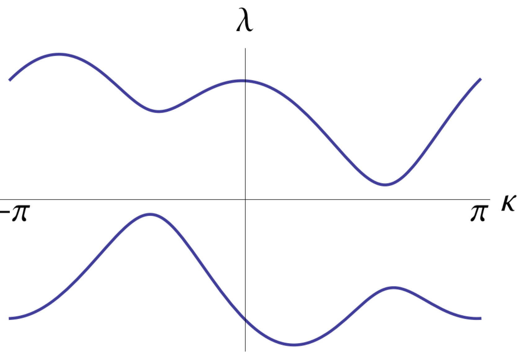

(a) 
(b) 
(c) 

Proof of Lemma 5.8. We discuss a typical case only. Let us first recall the base spaces of the two bundles, and , seen in Eq. (45): On the l.h.s. it is and on the r.h.s. . In a nutshell, we shall show that each side of the equation is associated with a cycle in or actually with a family of cycles parametrized by ; and, more precisely, with the bundle on of Lemma 8.2 restricted to that family. The proof then proceeds by an interpolation deforming one family into the other, up to contractible cycles. Most of the discussion occurs at fixed , which is hence once more omitted.
For on the l.h.s. of Eq. (45) the association is by (81) with . For on the r.h.s. a longer discussion is needed. The Bloch bundle (see Def. 5.6) can be analytically continued from real to the path , as long as is small enough. By there correspond two paths , in the sense that is a subcycle lying in the sheets of . Then
| (82) |
For the sake of illustration Fig. 7 shows the real energy curves , for various values of (left) next to the complex loops , with close to (right). The loops are understood on the observation that a portion of the energy curve increasing in is flanked by a nearby branch running in the upper half-plane. The loops can be mutually and self-intersecting, and intersect the spectrum. However the outer boundary of both loops does not. In the last case of Fig. 7 consists of two disconnected loops, each surrounding one of the bands , the second one being shown in Fig. 8, right.
The contour underlying may be picked as , at least in the cases where the latter is connected.
We claim:
Lemma 8.5.
The bundle contains a subbundle which is homotopic to the Bloch bundle . Moreover
| (83) |
where is a subcycle of the cycle . It covers twice.
As a result, is a cycle too, and
provides a complementary subbundle,
Lemma 8.6.
is contractible within .
As a result , and hence , are trivial.
This is the core of the proof of Lemma 5.8. In summary,
where is by homotopy or by dropping trivial subbundles. Some further comments in relation with Lemma 8.5 are appropriate.
First, one ought to worry about whether these equivalences persist once the dependence on is included into the picture. This will be understood by inspection of the proofs of the two lemmas. Indeed, the construction of , and hence that of , , will not involve any choices, except among homotopically equivalent constructions. In particular, as runs from to , the cycles match at the endpoints, whence the family glues up to tori; likewise for deformed cycles used in the interpolation.
Second, no deformation is needed at , see Fig. 7 (first case), where
| (84) |
Third, a cycle (parametrized by ) may give rise to a (i) torus (still called ) and to a (ii) bundle , which are both time-reversal invariant. For (i) it suffices that the map on leaves invariant. For (ii) the bundle, being of dimension , does not qualify as such. An additional structure is needed, namely an involution on preserving , which moreover commutes with . Then descends to the quotient , which consists of pairs of points related by the involution as well as by fixed points. Now shall actually stand for , whose fibers are, by continuous interpretation, of dimension even at fixed points. Both bundles and induce such involutions, on , resp. on : Points and are related by if ; and by if . We remark that are consistent with Eqs. (83, 82), respectively. At , where the cycles agree by (84), the involutions nevertheless differ. We will prove the homotopy in Lemma 8.5 by constructing cycles , interpolating between and . The bundle goes with the ride because of the following fact.
Lemma 8.7.
Let be as above. Then there is an interpolating involution on , commuting with .
8.1 Further details
Proof of Lemma 8.1. We expand the determinant (73) along the first row of blocks. Then, by the Laplace rule,
where contains only powers of of degree or higher. When looking for the leading term in we may replace by , which leaves an upper block triangular matrix. That term thus is . Similarly, the leading term in is . Eq. (74) follows from . In the time-reversal invariant case we use , where in the notation of Eq. (39). Hence the last claim.
Proof of Lemma 8.2. To be shown is that, for each , the eigenvalue of , cf. Eq. (41), is geometrically simple.
If the eigenvalue is even algebraically simple. In that case the eigenspace depends analytically on . If at , meaning a branch point, then we have by our general assumptions,
in particular is an eigenvalue of of algebraic multiplicity and , . It follows that nearby eigenvalues of are given as
| (85) |
In order to show that the geometric multiplicity of is nevertheless , we denote by the projection onto the group (85) of eigenvalues (it is analytic in ; [17], Sect. II.1.4), as well as by and by
the eigenprojection and eigennilpotent of . The claim amounts to , and we prove it by contradiction: implies that
has a removable singularity at . Hence , in violation of (85).
The proofs of Lemmas 8.5 and 8.6 will mostly deal with a single at a time and will be given them in two parts. The first part is, so to speak, a test run which avoids the complications due to the overlapping bands. It is thus restricted to the last case of Fig. 7 and pretends that even there. The limitations will be overcome in a second part.
Proof of Lemma 8.5, first part. We consider a homotopy of curves , which lie between and . In particular, we keep the endpoints of fixed, as indicated by the dashed line in Fig. 8 (right). Among the many curves in let us track the curve, , arising from at by continuity, i.e. . The curve has to stay outside of . Indeed, it can cross neither , as would end up inside , nor , as would approach from the outside. As does not penetrate into , it does not approach the real axis (i.e. ) on the branch of . Moreover it does not either on any other branch of , since those map to other, disjoint bands. That ensures that is a cycle in and that the bundle is defined and continuous in . Finally, the homotopy of bundles , does the job: For we have
by construction; for , and
Let us recall the count of preimages done in relation with Eq. (80). We find it convenient to pretend that all points , i.e. including , have precisely preimages under . This is enforced by including the preimages on , but by counting them with weight , as explained in the sequel of Eq. (77). The preimages of a loop intersecting the spectrum then is a pseudo-cycle, where it is tolerated that curves break up at pairs of points in with same (see the joined dashed and dashed-dotted curves in Fig. 8, left).
Proof of Lemma 8.6. We first observe from the previous proof that any point inside has preimages outside of and away from . We next extend from to so that it contracts to a point inside of it. We then consider the deformation , of pseudo-cycles covering twice and starting with . By continuity in , moves inside of , while preimages of remain outside. As a result stays away from and is a cycle in .
Proof of Lemma 8.5, second part. We extend the proof to general values of . They are illustrated by the three cases seen in Fig. 7 with the middle one having three variants (a–c). The argument will rely on two sheets () of , as opposed to just one before (see Fig. 8 left). Each comes with an annulus in bounded above by . The sheets share two branch points: In the first case ( or ) they rather are, to be precise, two double points at and . In the variant (a) each of them gives way to two branch points, out of which one is in , and actually in the annuli; in (b) the branch points have reached the paths (this might occur at different for the two points), and in (c) they have left the annuli. This is seen in Fig. 7 (right) as a rearrangement of loops through an intersection point at (b). It should be noted that the Bloch bundle with fibers remains continuous as the branch point reaches the paths , at least if properly interpreted: That point is then common to the two paths, resulting in a just 1-dimensional fiber, cf. Lemma 8.2; however the 2-dimensional fiber has a limit at the branch point, as remarked after Eq. (85), and unlike the two spanning vectors individually. That limit provides the appropriate fiber at the branch point.
In the first case of Fig. 7, where the curves do not intersect the spectrum, the conclusion is reached as before, but without need for deformations. We next turn to the three variants (a–c) of the middle case. Let us specify the deformations of the curves in and describe their lifts in .
(a-b) We deform the inner parts of the curve till they reach the outermost parts , while keeping the intersection points fixed. By the same arguments as before the preimage selected by continuity remains outside the annuli of both sheets.
(c) Let us expand the inner loops. Quite soon the situation will look as in the undeformed variant (b) with the inner loops touching essentially the same curves as they did there. By continuity from (b) the touching also takes places between their respective lifts in . From there on the deformation proceeds as in variant (b). As a whole it includes and reverts the rearrangement of loops which occurred between (a) and (c).
In the last case we first perform the deformation described in the first part of this proof. The two components of , which at this point are run through twice, still require a deformation to a countour encircling both bands at once. When the two components of first touch, so do the two lifts of each, as inherited from (c) by continuity.
Likewise the proof of Lemma 8.6 extends to the other cases, too. In the first case () the loops () are to be chosen so that .
Proof of Lemma 8.7. We begin with some preliminary observations about circle homeomorphisms , . Their degree is and any two of them are homotopic iff they have the same degree (); if so, the homotopies , between them fall into connected components which, relatively to one another, are labeled by . Indeed, for and fixed the map has a winding number (independent of ).
Continuous maps are called involutions if . They are homeomorphisms. Involutions have either all or no points as fixed points, or else just two [23]. The two cases correspond to , respectively. The above statements about homotopy remain true within the class of involutions.
We remark that the properties to be proven,
| (86) |
are relations within or between the fibers at and , respectively.
We first consider the cases . There the cycle is independent of and consists of two loops with the involution , (see (75, 76)) interchanging them. Maps are expressible in terms of and properties (86) are (jointly) equivalent to , ; actually the latter property just determines in terms of . It is clear from the definitions of that they satisfy (86). Moreover it is impossible that for some , since that would imply , in contradiction with . Hence has no fixed points. But that map equals , whence and . Therefore there is an interpolation , with satisfying (86). In addition, there are more of them, differing from it by any given winding .
We now turn to . The second property (86) will simply determine at in terms of its value at . Hence only the first one matters in the following construction of , . To begin, for (i) near the cycle can still be identified with ; further on it may (ii) collapse into a ”figure 8” (for this occurs when a single branch point intersects ; but does not for ), and thereafter (iii) become a single loop. Eventually, the cycle reverts to two separate loops before reaches . In range (i) ought to interchange the two loops and (86) just determines in terms of . That half of can simply be chosen by continuity from . At (ii) continuity requires that the intersection point be a fixed point of , which can be arranged for on the side of (i). In the range (iii) is an involution on a single loop with just two fixed points. At the end of that range, the two fixed points are again to coalesce into an intersection point, but that does not obstruct the construction of (see the observations at the beginning of the proof).
The whole construction could have begun from instead. We have to ensure that the two interpolations constructed from the two ends match at some . This can be arranged, because their relative winding can be chosen to vanish.
9 Bulk-edge correspondence through scattering theory: Proofs
Proof of Lemma 6.7. i) The map is well-defined by the required properties, and it remains to show that it is real analytic in . Away from critical points, , let , so that . Since for , the claimed analyticity follows by the implicit function theorem. Near a critical point, say , the argument must be modified. Let there
Note that still has the solution , but no longer , except for . Since
equals at the solution is analytic also near .
ii) We recall the Def. 6.5 of the Bloch bundle . As shown in Fig. 5, does not contain any non-contractible loop winding around . Thus there is no obstruction for a smooth section of on , or even on small complex neighborhood in thereof. To be shown is that there is one, , which at fixed is analytic in for in that neighborhood. As a preliminary, let be the Riesz projection onto the fiber ,
where is defined in Eq. (41), the variable is suppressed, and the integration contour surrounds once the eigenvalue of , and no further ones. We observe that is analytic in .
We construct first by setting for, say, ; then by extending it in (at fixed ) through parallel transport:
| (87) |
This is feasible. In fact, the ansatz
reduces both equations to
Here for some function , since the fibers are lines. The equation thus reads , which can be integrated starting from . It remains to verify the Cauchy-Riemann condition . By the Eqs. (87) and we indeed have .
In preparation for the proof of Lemma 6.8, or actually of an extension thereof, let us list two further properties of the Casoratian, Eq. (60). This time, the energy in Eq. (61) is real.
- C4)
Let be a Bloch solution of quasi-periodicity , and energy . Then
(88) - C5)
Let be a Bloch solution as in (C4) for near . Then is a generalized Bloch solution by Lemma 8.4 and
(89)
The derivation is as follows. We recall that in Eq. (39) satisfies Eq. (41) with . Eq. (79) thus yields the Feynman–Hellmann equation
by , the inner product being the standard one on . The l.h.s. equals
as claimed in (C4).
Differentiation of (88) yields (89) because of and .
Let us consider a complex neighborhood of the band under consideration:
The following lemma manifestly implies Lemma 6.8, which therefore will not require a separate proof.
Lemma 9.1.
[Solutions of at most small exponential growth] For small enough there is such that we have: For there is (up to multiples) a unique solution of
with , . It is of the form
| (90) |
where
| (91) |
and
- i)
for : , are Bloch solutions for with , resp. ;
- ii)
for : , are Bloch, resp. generalized Bloch solutions with .
Moreover, if , ), then and in case (i); and in case (ii).
Proof. At first, let belong to the band under consideration, i.e. , ). As explained in connection with the Bloch variety Eq. (76), we have for values of with (counting multiplicities) and for values with and small enough . By possibly making it smaller the same remains true for and small , provided is replaced by . Any eigensolution of , which remains , is thus of the form
| (92) |
where is a (generalized) Bloch solution corresponding to the above ’s, in the stated order. Disregarding the boundary condition, the same applies to eigensolutions of for , by means of the map (28).
We claim that up to multiples there is precisely one such solution , once the boundary condition is imposed. Without any conditions the space of solutions has dimension . The subspaces determined by , resp. , have dimensions , . Their intersection thus has dimension at least . We make two claims: , cf. (90), which implies Eq. (91) and ; and the stronger: , and hence , which is the statement of uniqueness of . Properties are stable, because the nullity of a pair of subspaces is an upper semi-continuous function of them ([17], Thm. IV.4.24); hence it suffices to prove them for with real.
We begin with : The opposite would amount to an embedded eigenvalue, which is ruled out by (51). To prove , together with the remaining claims, we consider first the case , where are different. Suppose, indirectly, . Then, by taking a suitable linear combination of solutions we could arrange for , (or viceversa). This would imply the contradiction
by and the preliminary remark (C4). Finally we are left with (or ). This time would imply that there exist two solutions : one with , in Eq. (92) and the other with , . The resulting contradiction is
by (C5) and .
Moreover, the bounds and follow from Eqs. (40, 78) with .
Proof of Lemma 6.10. Let again be fixed till further notice. We consider in a complex neighborhood of the upper band edge . There the expanded part of the solution (90) may alternatively be written as a linear combination of
where is the section of Bloch solutions of Lemma 6.7 (ii), rather than as linear combination of Bloch solutions , . The advantage of the basis is that it does not degenerate as . The solution (90) is unique up to a multiple, which we shall fix by means of a prescription independent of . For instance, since , there is a linear functional on such that for near . We impose the normalization . We then have
| (93) |
with analytic near . Moreover, are even under since , , are. A semi-bound state is tantamount to . For we may also write
where
| (94) |
is analytic in a punctured neighborhood of . Comparison with Eqs. (52, 53) yields for later use
| (95) |
For the Bloch solution is exponentially diverging for due to . Based on , edge state energies close to occur iff for some close to with . For that to happen has to be correspondingly small:
| (96) |
Let us now reintroduce the parameter of the lemma and of its assumption Eq. (54). Then follows by continuity. This concludes the proof.
Proof of Theorem 6.11. Let us first deal with the simple case that the interval does not contain any where has a semi-bound state. Then vanishes by Lemma 6.10 and so does the l.h.s. of Eq. (55). In fact, by (94, 95) we have
uniformly in , since . We consider next the case where such points are present. Though they are generically isolated, we will treat the general case, where they form intervals . Those are closed, countably many and possibly consisting of single points. By the first case and by compactness it suffices to consider such an interval and sufficiently close to its endpoints.
Let first . Then , since ; see Eq. (93). We claim there is a punctured disk of fixed radius centered at , which remains free of zeros of . Indeed, if that radius is small, Eq. (96) can not hold true there, because its r.h.s. is linearly large in , while the l.h.s. is quadratically small, as is even. The claim extends by continuity to , provided the punctured disk is replaced by an annulus of fixed radii.
We recall that by (51) real do not occur as zeros either. Let be the number of zeros inside the annulus and having . Thus
Eq. (55) then follows from the claim that
| (97) |
In proving it we drop from the notation, e.g. . We note that by assumption , whence there is a disk centered at which is free of zeros of . In particular, for small , and for suitable ; likewise for the images under , see Fig. 9.
We consider the contour , where , joins to , and joins to . Let us denote by that contour with opposite (positive) orientation. By the argument principle we have
The contour may also be split into two parts, and their contributions computed otherwise. First, by (95)
(Note that the first equality is consistent with being a continuous argument in ; so is the second, because the path remains free of zeros as changes, unlike ). Second, by Eq. (94)
Together, this proves (97) and hence the theorem for the upper band edge. The case of the lower band edge is similar, except that incoming states are found at . This explains the reversed count of signs in .
Proof of Proposition 6.12. We write only when necessary. Since is a non-degenerate maximum, the energy curve bijectively maps a neighborhood of in the half-plane to one of the band edge , however slit by the band itself. It will be understood that and are so related. We first consider the case of a disappearing branch and reformulate the statement using the notation from the proofs of Thms. 6.11 and 5.4. Since no eigenvalue branch is present at , the two sides of Eq. (56) are, after dividing by , those of
| (98) |
where
- •
is the contour in the -plane described in Fig. 9;
- •
is the contour encircling the crossing point with the Fermi line and described in Fig. 4;
- •
has an eigenvalue iff (with both zeros being of first order), since both conditions are equivalent to . Hence Eq. (98) holds provided the contours are homotopic under .
To show this, let us visualize in the setting of Fig. 1. That contour can be rotated without intersecting the discrete eigenvalue branch, and so as to lie in a -plane at fixed . The contour remains positively oriented w.r.t. the orientation of that plane and, after substitution , it is homotopic to at .
In the case of an emerging eigenvalue branch, the l.h.s. of (98) is evaluated at and acquires a minus sign, cf. (56). However, when is rotated as just prescribed it ends up negatively oriented in the -plane at . Hence the modified Eq. (98) still holds.
Acknowledgments. We thank Y. Avron, C. Cedzich, M. Fraas, J. Fröhlich, H. Schulz-Baldes, and D. Würsch for discussions. The work of M.P. is supported by the Swiss National Science Foundation.
References
- [1] Avila, J.C., Schulz-Baldes, H. and Villegas-Blas, C.: Topological invariants of edge states for periodic two-dimensional models. arXiv:1202.0537
- [2] Bernevig, B.A., Hughes, T.L. and Zhang, S.-C.: Quantum spin Hall effect and topological phase transition in HgTe quantum wells. Science 314, 1757-1761 (2006).
- [3] Bräunlich, G., Graf, G.M. and Ortelli, G.: Equivalence of topological and scattering approaches to quantum pumping. Commun. Math. Phys. 295, 243-259 (2010).
- [4] Essin, A.M., Gurarie, V.: Bulk-boundary correspondence of topological insulators from their Green’s functions. Phys. Rev. B 84, 125132 (2011).
- [5] Fröhlich, J. and Kerler, T.: Universality in quantum Hall systems. Nucl. Phys. B 354, 369-417 (1991).
- [6] Fröhlich, J. and Studer U.M.: Gauge invariance and current algebra in nonrelativistic many-body theory, Rev. Mod. Phys 65, 733 (1993).
- [7] Fröhlich, J., Studer U.M. and Thiran, E.: Quantum theory of large systems of non-relativistic matter, Les Houches Lectures 1994, Elsevier (1995); arXiv:cond-mat/9508062.
- [8] Fröhlich, J. and Zee A.: Large scale physics of the quantum Hall fluid. Nucl. Phys. B 364, 517-540 (1991).
- [9] Fu, L. and Kane, C.L.: Time reversal polarization and a adiabatic spin pump. Phys. Rev. B 74, 195312 (2006).
- [10] Fujita M., Wakabayashi K., Nakada K. and Kusakabe K.: Peculiar localized state at zigzag graphite edge. J. Phys. Soc. Jpn. 65, 1920-1923 (1996).
- [11] Haldane, F.D.M: Model for a quantum Hall effect without Landau levels: Condensed-matter realization of the “parity anomaly”. Phys. Rev. Lett. 61, 2015-2018 (1988).
- [12] Hasan, M.Z. and Kane C.L.: Topological insulators. Rev. Mod. Phys. 82, 3045-3067 (2010).
- [13] Hatsugai, Y.: Chern number and edge states in the integer quantum Hall effect. Phys. Rev. Lett. 71, 3697 (1993).
- [14] Hatsugai, Y. and Ryu, S.: Topological origin of zero-energy edge states in particle-hole symmetric systems. Phys. Rev. Lett. 89, 077002 (2002).
- [15] Hsieh, D., Qian, D., Wray, L., Xia, Y., Hor, Y.S., Cava, R.J. and Hasan, M.Z.: A topological Dirac insulator in a quantum spin Hall phase. Nature 452, 970 (2008).
- [16] Kane, C.L. and Mele, E.J: Topological order and the quantum spin Hall effect. Phys. Rev. Lett. 95, 146802 (2005).
- [17] Kato, T.: Perturbation Theory for Linear Operators. Springer-Verlag (1980).
- [18] Kohn, W.: Analytic properties of Bloch waves and Wannier functions. Phys. Rev. 115, 809-821 (1959).
- [19] König, M., Wiedmann, S., Brüne, C., Roth, A., Buhmann, H., Molenkamp, L.W., Qi, X.-L. and Zhang, S.-C.: Quantum spin Hall insulator state in HgTe quantum wells. Science 318, 766 (2007).
- [20] Moore, J.E. and Balents, L.: Topological invariants of time-reversal-invariant band structures. Phys. Rev. B 75, 121306(R) (2007).
- [21] Nakada, K., Fujita, M., Dresselhaus, G. and Dresselhaus, M.S.: Edge state in graphene ribbons: Nanometer size effect and edge shape dependence. Phys. Rev. B. 54, 17954 (1996).
- [22] Nakahara, M.: Geometry, Topology and Physics. Graduate Student Series in Physics, Institute of Physics Publishing (1990).
- [23] Pfeffer, W.F.: More on involutions of a circle. Amer. Math. Monthly 81, 613 (1974).
- [24] Prodan, E.: Robustness of the spin-Chern number. Phys. Rev. B 80 , 125327 (2009).
- [25] Qi, X.-L., Wu, Y.-S. and Zhang, S.-C.: Topological quantization of the spin Hall effect in two-dimensional paramagnetic semiconductors. Phys. Rev. B 74, 085308 (2006).
- [26] Reed, M. and Simon, B.: Methods of Modern Mathematical Physics, III. Scattering Theory. Academic Press (1979).
- [27] Roy, R.: classification of quantum spin Hall systems: An approach using time-reversal invariance. Phys. Rev. B 79, 195321 (2009).
- [28] Schulz-Baldes, H., Kellendonk, J. and Richter, T.: Simultaneous quantization of edge and bulk Hall conductivity. J. Phys. A: Math. Gen. 33 L27 (2000).
- [29] Sheng, D.N., Weng, Z.Y., Sheng, L. and Haldane, F.D.M.: Quantum spin-Hall effect and topologically invariant Chern numbers. Phys. Rev. Lett. 97, 036808 (2006).
- [30] Thouless, D.J.: Quantisation of particle transport. Phys. Rev. B 27, 6083-6087 (1983).
- [31] Wen, X. G.: Chiral Luttinger liquid and the edge excitations in the fractional quantum Hall states. Phys. Rev. B 41, 12838–12844 (1990).
- [32] Zhang, S.-C.: The Chern-Simons-Landau-Ginzburg theory of the fractional quantum Hall effect. Int. J. Mod. Phys. B 6, 25-58 (1992).