From billiards to thermodynamics
Abstract
We explore some beginning steps in stochastic thermodynamics of billiard-like mechanical systems by introducing extremely simple and explicit random mechanical processes capable of exhibiting steady-state irreversible thermodynamical behavior. In particular, we describe a Markov chain model of a minimalistic heat engine and numerically study its operation and efficiency.
1 Introduction
The main purpose of this paper is to introduce a class of simple random mechanical model systems that may help in shedding light on the mechanisms whereby steady state, out of equilibrium thermodynamical behavior can emerge in random dynamics. In the spirit of classical statistical mechanics, our random systems arise as a certain form of course-graining of Hamiltonian mechanical models; among these models we look to the simplest ones, in which all the interactions are through elastic collisions, namely billiard systems.
We shall interpret the term “emerging thermodynamical behavior” rather concretely by considering the problem of obtaining a random mechanical system that can perform at steady-state (stationary) mode as a heat engine, defined in an explicit fashion using few degrees of freedom.
The main motivation lies in the belief that a rich collection of model systems that are amenable to detailed numerical and analytical exploration is essential to guiding the development of a stochastic theory of non-equilibrium thermodynamics. See [5] for the mathematical outlines of such a theory. For a more applied perspective see, e.g., [13, 14] and related literature on stochastic thermodynamics. Our main contribution here is to describe purely mechanical, billiard-like stochastic (Markov chain) processes, obtained by a specific form of coarse-graining from deterministic billiards, built from a rather small number of parts and fully explicit in a sense to be clarified later in the paper, which can exhibit (in the mean) textbook thermodynamical behavior. In particular, we describe a minimalistic billiard-Markov heat engine capable of producing mechanical work in a steady-state regime of operation.
Related studies in the stochastic thermodynamics literature, or in numerical studies of molecular motors and models of Feynman’s ratchet and pawl system (such as in [16]), typically start from a Langevin equation and the a priori existence of a heat bath at a given temperature. A distinguishing feature of the present work is that we have an explicit Markov model of the heat bath-thermostat, which is very closely related to the deterministic system from which it is derived. Our systems are examples of random billiards, a term that will be expanded upon later in the paper. (See also [4, 7, 8].)
The paper is organized as follows. In Section 2, the most basic facts about (deterministic) billiard dynamical systems are recalled for later use. These are mechanical systems in which the interaction between moving parts is limited to elastic collisions; in particular, there are no potentials or dissipative forces. The section lingers a bit on a description of the natural flow invariant measure in the phase space of the billiard system, emphasizing the so-called cosine law for billiard reflections. As a prelude to introducing our billiard thermostat later in Section 3.2, we also show in Section 2 how the Maxwell-Boltzmann distribution of velocities is obtained from the cosine law and a simple (well-known) geometric argument concerning the phenomenon of concentration of volumes in high dimensions.
Section 3 introduces the idea of random billiard systems. These are Markov chain systems with general (i.e., not necessarily countable) state spaces obtained from deterministic billiards (see Section 2) by the following general method. We select one or more dynamical variables of a given deterministic mechanical system and turn them into random variables with fixed in time probability distributions. It is natural to choose for the latter the asymptotic probability distribution that those variables attain in the original deterministic system. The resulting random dynamical system is often not far removed, in certain ways, from the deterministic system that gave rise to it. For example, for the main class of random billiards described in Section 3, the velocity factor of the flow-invariant measure in phase space becomes a stationary measure for the associated random process, suggesting that the random and deterministic systems have closely related ergodic theories.
Also in Section 3 we introduce and explore a random billiard system that will serve as our all-purpose heat bath-thermostat. It is indicated there (and proved in [4]) that a sequence of collisions of a point mass with the random billiard thermostat yields a Markov chain process (in the state space of post-collision velocities) whose stationary distribution is Maxwell-Boltzmann’s. Thus, in our systems, thermostatic action is not imposed by fiat but modeled explicitly. As already noted, this is a distinguishing feature of our models.
All pieces will then be in place to study heat flow between two billiard thermostats at different temperatures. This is done in Section 4. The basic mechanism of operation of a heat engine already becomes apparent at this point. In Subsection 4.2 we propose a particular design for such an engine which is as simple as we could conceive. The associated random billiard is -dimensional, that is, it contains moving parts (point masses): one “gas molecule,” one “Brownian particle,” an additional particle that acts as an “escape valve” to the gas molecule, and two masses for the two thermostats at different temperatures. The whole contraption is essentially one-dimensional in physical space. We briefly explore the engine’s operation by numerical simulation and compute the mean velocities of rotation and the engine’s (rather modest, but positive) efficiency for different values of a force load.
2 Deterministic billiards
A brief overview is given here of the most basic properties of deterministic billiards needed for our discussion of random billiards in the next section. Most importantly, is a description of the billiard flow-invariant volume in phase space and the so-called cosine law for billiard reflection.
2.1 Basic facts
Billiard systems, broadly conceived, are Hamiltonian systems on manifolds with boundary, the boundary points representing collision configurations. Most commonly, the configuration manifold is a region in the Euclidean plane having piecewise smooth boundary, although higher dimensional systems are widely studied and will be encountered throughout this paper. Higher dimensional billiards typically describe mechanical systems consisting of several rigid constituent masses interacting only through collisions. The configuration manifold is endowed with the Riemannian metric defined by the kinetic energy bilinear form. In particular, the (linear) collision map at boundary points of the configuration manifold is a linear isometry under the assumption of energy conservation. The collision map is often taken to be the standard Euclidean reflection, that is, a map that fixes all the vectors tangent to the boundary while sending a vector perpendicular to the boundary to its negative. In this paper the Riemannian metric on configuration space will always have constant coefficients (associated to masses of the constituent rigid parts of the system) and so will be an Euclidean metric.

Figure 1 shows two famous examples of the basic kind of billiard system. In each case, the billiard table is a planar region whose boundary consists of piecewise smooth curves; the billiard particle undergoes uniform rectilinear motion in the interior of the region, bouncing off specularly after hitting the boundary.
In general, let denote the billiard’s configuration manifold. This is the planar regions in the -dimensional examples of Figure 1. The phase space is the bundle of tangent vectors on which one defines the flow map . The flow map assigns to each time and tangent vector the state (i.e., the position and velocity) of the billiard trajectory at time having initial conditions at time .
It will be assumed here that the billiard particle is not subject to a potential function or any form of interaction other than elastic collision. For a more general perspective see [4]. Thus the speed of billiard trajectories (given in terms of the mechanically determined Riemannian metric) is a constant of motion, usually arbitrarily set to , and the flow map is often restricted to the submanifold of unit vectors in . The precise definition of the billiard flow contains some important fine print, dealing with the issue of singular trajectories; for example, those trajectories that end at corners or graze the boundary of . For the omitted details (in dimension ) see [3].
A fact of special significance is that the billiard flow map leaves invariant a canonical volume form on phase space. There is also an associated invariant volume form on the space of unit vectors on the boundary of . The existence of these invariant volumes is fundamental for the ergodic theory of billiard systems and for the probability theory we wish to employ later, so we take a moment to describe them in detail.

Let be the dimension of and the subset of consisting of unit vectors at boundary points of pointing towards the interior of . Then is the disjoint union of hemispheres defined at each . The unit normal vector is contained in ; we denote by the angle between a given and and by the -dimensional volume element at over . Also let denote the volume element at on the boundary of (associated to the induced Riemannian metric). The billiard flow induces a map on as follows: for each write , where is the moment of next collision with the boundary; then , where indicates the reflection of back into . We refer to as the billiard map. The transformation is said to preserve, or leave invariant a measure on if (writing )
for every integrable function . The next proposition is well-known.
Proposition 1.
leaves invariant on the measure element
| (2.1) |
For a proof (of a more general expression) under much more general conditions that allow for potentials and non-flat Riemannian metrics see [4].
The existence of this invariant measure on is the starting point of the ergodic theory of billiard systems. We always assume that the measure is finite and typically rescale it so that ; in this case it is natural to interpret as a probability measure. A billiard system is said to be ergodic if cannot be decomposed as a disjoint union of two measurable subsets, both invariant under and having positive measure relative to . Ergodicity can also be expressed in terms of the equality of time and space means:
| (2.2) |
where is any integrable function on . (See [11] for a general reference for ergodic theory as a chapter in the mathematical theory of dynamical systems.) The existence of the limit, and the equality in 2.2 under the ergodicity assumption, is the content of the celebrated ergodic theorem of Birkhoff. Below, we refer to the identity itself as the ergodic theorem.

Proving that a billiard system is ergodic is generally a technically difficult task. In fact, a significant part of the general theory of dynamical systems, particularly hyperbolic (strongly chaotic) systems, has been developed in pursuit of establishing ergodicity for such statistical mechanical systems as hard spheres models of a gas. (See, e.g., [1] or [2], chapter 8.)
An immediate consequence of the ergodic theorem is that the long term distribution of post collision angles of an ergodic billiard in any dimension satisfies the cosine law, whereas the distribution of collision points on the boundary of is uniform relative to the measure . More precisely, let be the velocities immediately after collisions registered at each moment that a billiard trajectory returns to a segment of the boundary of having positive measure. Then for almost all initial conditions the set of angles is distributed according to , where is a normalizing constant and the angle brackets denote inner product and , where is the angle between and .
2.2 Illustrating the cosine law with a variant of Sinai’s billiard
The billiard table of Figure 4 represents a container divided in two chambers by a porous solid screen composed of small circular scatterers. The scatterers are separated by small gaps. A billiard particle represents a spherical gas molecule. One is interested, for example, in how a “gas” consisting of a large number of billiard particles injected at time into, say, the left chamber, will expand to fill up the entire container.
This billiard table can be regarded as an “unfolding” of Sinai’s billiard shown on the left of Figure 1, and from this observation it can be shown that the associated billiard flow is ergodic. Figure 4 shows one long segment of trajectory, indicating the initial velocity vector and the image of that vector under the billiard flow at time . This is an example of a (semi-) dispersing billiard, which are well-studied models of chaotic dynamics (see [3]). Trajectories are highly unstable in their dependence on initial conditions due to the presence of the circular scatterers.

Consider Figure 5, where we focus on one fundamental cell of the solid screen. We define the reduced phase space of this system as the set
A state of the form gives the initial condition of a trajectory that enters into the scattering region from the left () or the right () chamber at a position in the interval , with velocity , where and are the standard basis vectors of . The reduced billiard map then gives the end state of a trajectory that begins and is stopped at . The billiard motion on the full table is an appropriate composition of with a similar return map on a rectangular table.

Given a long trajectory of a billiard particle, we register the values in , which is the sequence of sides of the container the particle occupies at each moment it enters the scattering region; in , the sequence of positions along the flat boundary segments of the fundamental cell at which the particle enters the region; and in , the sequence of angles the particle’s velocity makes with the normal vector to those boundary segments. A remark about the first sequence will be observed shortly; first note that the long term distribution of the is uniform along the unit interval. This follows from the above observation on the form of the invariant measure and the ergodic theorem, and is observed in the numerical experiment of Figure 6.

The distribution of the angles is given, as expected, by the cosine law. This is shown in Figure 7. For ergodic polygonal billiards these long term distributions of positions and angles hold, but convergence is much slower.
Figure 8 shows the result of releasing a large number of independent (i.e., that do not collide with each other) billiard particles at into the left chamber of the container. The solid line graph gives the fraction of particles in the right chamber as a function of time. (Time is expressed in arbitrary units of length divided by . Recall that the speed is set equal to .) The other graphs are explained later. (Section 3.)

The salient point this graph dramatizes is the issue of time reversibility versus irreversibility. In the long run the fraction of particles in each chamber appears to stabilize to , as our physical intuition would suggest. This behavior of the system of many particles introduces a sense of direction of passage of time that is not present in the time reversible nature of the billiard dynamic. The issue of explaining irreversible behavior in the collective motion of a large number of particles whose fundamental evolution is time reversible is a central problem in non-equilibrium statistical physics. This so-called arrow of time problem, of deriving macroscopic irreversibility from microscopic reversibility, has bedeviled the study of statistical mechanics since its beginnings in Boltzmann’s fundamental work in the early 1870s. In fact, one early objection to Boltzmann’s work is the so-called Zermelo’s paradox [15], which is based on a fundamental observation of H. Poincaré known as Poincaré’s recurrence (see [11] for its abstract, measure theoretic form) implying that, with probability on the initial conditions, there will be an infinite sequence of times when those particles all come together back into the initial chamber on the left. We refer the reader to the vast literature on the Boltzmann equation and the -theorem for more information on this topic.

The cosine distribution of angles has great significance in kinetic theory of gases and gas diffusion, particularly in the so-called Knudsen regime of rarified gases, when transport properties are more strongly affected by collisions between gas molecules and the walls of the container than by collisions between the molecules themselves. The appearance of the cosine term in the scattering distribution of gas molecules was studied experimentally by M. Knudsen in the early years of kinetic theory. His experiments are described in [12]. In many texts, particularly in engineering, the cosine distribution is often referred to as Knudsen’s cosine law. See [6] for further information.
2.3 A geometric remark about many particles systems
The single particle billiard system is a geometric representation of a mechanical system that may consist of many constituent rigid particles interacting with each other through elastic collisions. This simple remark is immediately understood by considering the two-particle, one-dimensional billiard system shown at the top of Figure 9.
To be fully specified, the billiard table must be given a Riemannian metric relative to which reflections are specular. The triangular region of Figure 9 with the standard Euclidean inner product does not in general define a billiard system since if , the single particle in the triangle, whose and coordinates give the positions of the two masses along the interval , will not reflect specularly when colliding with the diagonal side of the triangle. A simple way to make the collision specular is to absorb the mass values into the position coordinates. Thus we define coordinates where , and note that the kinetic energy of the system, expressed in the new coordinates, is a constant multiple of the ordinary Euclidean norm. Therefore, a linear transformation that conserves energy becomes an orthogonal map. Conservation of linear momentum means that the component of the pre-collision velocity vector in the direction of the slanted side of the triangle in the new metric equals the same component for the post-collision velocity. Therefore, the normal component of the pre- and post-collision velocities can only be either equal or the negative of each other. Obviously, the latter must the case as there would be no collision otherwise.

These new, mass-rescaled coordinates yield a bona fide billiard system on the plane. We call the single particle system in the triangular region with the new metric the billiard representation of the one-dimensional two-particle system. The idea is obviously very general and works in any dimension, for any number of masses. In higher dimensions, say, for the collision of two solid bodies in -dimensional space, the basic conservation laws of energy, linear and angular momentum, as well as the imposition of time-reversibility and linearity, do not fully specify the collision map. Further assumptions about the nature of contact, such as being slippery or rubbery, are needed.
2.4 Knudsen implies Maxwell-Boltzmann
One has not entered thermodynamics until temperature is somehow brought into the picture, and for our needs this may be done via the Maxwell-Boltzmann distribution of velocities. In the present section we illustrate with a simple example the geometric explanation of how this fundamental distribution arises in the context of billiard dynamics. This discussion serves to motivate our model of random billiard thermostat that will be introduced in Section 3.2 and is not strictly necessary for defining the billiard heat engine of Section 4.2. The reader who wishes to skip this section on first reading may do so without great loss of continuity.

The example is shown in Figure 10. It consists of point masses that can slide without friction on a line. Masses are restricted to lie in the interval and they move independently of each other. Their position coordinates are indicated by ; can move in the bigger interval , with position coordinate . At the endpoints of the bounce off elastically. Mass moves freely past (dashed line in Figure 10), and it collides elastically with the and with the wall at . We imagine the as tethered to the left wall by inelastic and massless, but fully flexible strings of length ; when the strings are stretched to the limit of their length, the masses bounce back as if hitting a solid wall at .
To make the system more symmetric without changing it in any essential way, we regard the wall on the left as a mirror and we keep track of both and its image ; thus can be negative. (The thickness of the masses is considered negligible in this model.) In this symmetric form, the billiard representation of the system is as shown in Figure 11.
Let . Changing coordinates to
the kinetic energy form becomes
We may equivalently assume that defines a point on the hypercube with coordinates in , where , having in mind the above comment about mirror image. Mass is then constrained to move on the interval where

Thus the configuration manifold is
and collision is represented (due to energy and momentum conservation and time-reversibility), by specular reflection at the boundary of . We now wish to follow the motion of mass ; geometrically, this amounts to following the image of billiard orbits under the orthogonal projection , as indicated in Figure 12. In particular, what can be said about the distribution of values of the projection of the velocity of typical billiard trajectories over long time spans? The following elementary proposition points to an answer.
Proposition 2.
Let denote the hemisphere of dimension and radius , consisting of vectors such that and . Let be the Knudsen cosine probability measure on ; thus , where is the Euclidean volume measure on and is a normalizing constant. Let be the image of under the projection map . Thus the -measure of an interval is, by definition, . Then, as goes to infinity, the sequence of converges (in the vague topology of probability measures) to on such that
| (2.3) |
We refer to as the post-collision Maxwell-Boltzmann probability measure in dimension , with parameter . Similarly, let be the probability distribution of , , given that is distributed according to . Then in the limit as approaches infinity converges to the Gaussian
| (2.4) |
Proof.
For convenience set and let be the unit -sphere in centered at the origin. Let be the polar coordinates map on the hemisphere, which is defined by
Let denote the volume form on the -dimensional hemisphere of radius and the volume form on the unit sphere of dimension . A geometric exercise yields the expression of in the just defined coordinates as
Given now any bounded function on the interval , we obtain by a change of variables in integration that
Integrating over the unit -sphere in the last integral gives, for a new constant ,
Reverting back to and using that converges to as tends to infinity, finally gives (for yet another constant independent of )
As is arbitrary we conclude that
The constant is easily found to be by normalization. The claim for the other components of is similarly demonstrated. ∎
Proposition 2 is a manifestation of the well-known connection between probability theory (and statistical physics) and geometry in high dimensions. An especially intriguing exposition of this connection under the heading of concentration of measures may be found in [9], chapter .

The appearance of the Maxwell-Boltzmann (MB) distribution in our billiard model can now be explained as follows. Observing the velocity of the mass amounts to taking the projection of the velocity of the billiard trajectory as in Figure 12; if the billiard system is ergodic (this depends on the ratios of masses, although as far as we know there is no general criterion of ergodicity for polyhedral billiard tables, even in dimension ), then as indicated earlier the long term distribution of velocities at the moments when the billiard particle emerges from the interaction zone on the left-hand side of the polyhedral table follows a cosine distribution. The proposition now implies that the projections should then follow the approximate MB distribution for finite . The approximation becomes better as the number of masses near the wall of the system of Figure 10 increases and the total energy increases proportionally.
Reverting to the initial velocity variables (i.e., before we absorbed the masses to form the above ) and indicating by the velocity of , the post-collision MB distribution can be written as
| (2.5) |
where is a parameter with units of energy. Later on, after we introduce our random billiard model for a thermostat, we will remark on how equality of for two parts of a system is a necessary condition for stationarity, so we recover the idea of thermal equilibrium. In statistical physics ones writes , where is the so-called Boltzmann constant and is absolute temperature.
Notice the difference between what we have called above the “post-collision” MB distribution and the MB distribution for the particle’s velocity sampled at random times, in which case the velocity can be both positive and negative. If is the post-collision density shown in 2.5, then at a random time each velocity should be weighted by the time the particle, having this velocity, takes to go from one end of the interval to the other, which is proportional to . This term cancels out the factor in , yielding the standard one-dimensional MB-distribution 2.4.
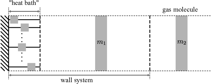
We point out for later use the model of Figure 13 of thermal interaction between gas molecule and wall. The masses on the far left have a very short range of motion, limited by the first dashed line, compared to , which is limited by the second dashed line on the right. The gas molecule, , can move across those lines. As discussed above, when the number of masses constituting the finite “heat bath” grows, the asymptotic distribution of positions of (under the assumption of ergodicity) becomes uniform and the distribution of velocities of becomes Gaussian. The random billiard thermostat to be introduced in the next section will be abstracted from this deterministic model by eliminating the masses on the left (the “heat bath”) and setting the statistical state of equal to the asymptotic distribution (of position and velocity) this mass would have in the deterministic system in the limit of very large .
3 Random billiard models and the billiard thermostat
Our thermodynamical systems will be defined as stochastic processes derived from billiard systems. The central concept is of a random billiard, explained below. After general definitions and motivations, we introduce a model thermostat, which is the key component in the construction of our heat engine in the next section.
3.1 Random billiards
A very current and active program in the ergodic theory of hyperbolic (chaotic) systems, in particular chaotic billiard systems, is dedicated to obtaining probabilistic limit theorems such as the central limit theorem for the deterministic system. This is a technical area of investigation, which we do not attempt to survey here. Our goal is to abstract from the billiard systems plausible random models that we can more easily study and of which more explicit results can be derived. Thus we now turn to the topic of random billiards.
The basic idea is as follows. Starting with a deterministic billiard system, we take some of its dynamical variables and assume that they are random variables with a given distribution. As will be seen in the specific examples, the resulting system is typically expressed as a Markov chain with non-discrete state space. The selection of variables and the choice of probability law assumed for them can vary, but we observe the following procedure: the probability law for a given random variable is taken to be the asymptotic distribution that that variable assumes in the deterministic system from which the random system is derived.
To illustrate this idea we return to the divided chamber example of Section 2.2. There are many possibilities for turning the original system into a random system; we first indicate an extremely coarse model and then show a much more refined one. The coarse model, which only serves a didactical purpose and is not going to be of further use, consists of a two-state Markov chain with state space , where stands for the left side chamber and for the right side one. We set a time unit equal to the mean time a billiard trajectory takes to return to the zone of scatterers and calculate (numerically) the transition probabilities of moving from one to the other chamber at each return. The resulting Markov chain is shown in diagram form in Figure 14.

The dot-dashed graph of Figure 8 shows the result of the experiment of releasing a large number of particles in one chamber and observing how long it takes for the distribution of particles to even out. The solid line gives the same distribution for the original deterministic system.
We now turn to the more refined model (Figure 15) which, as will be seen, preserves many of the geometric features of the original system. The screen of circular scatterers is replaced with a vertical line. Upon colliding with this line, the billiard particle changes both direction and chamber as prescribed by transition probabilities with state space where the first factor indicates as before the side of the divided container ( for left and for right) and the second factor gives the angle along which the particle impinges on or scatters off the dividing screen. Recall the deterministic map defined on the reduced phase space of the fundamental cell shown in Figure 5. The velocity and chamber of the billiard particle immediately after collision with the scattering line are then defined to be random variables obtained from and the pre-collision side and angle variables by letting the position be random, uniformly distributed over the unit interval.
To obtain the transition probabilities operator, we refer back to the notation set in Figure 5. We wish to describe the transition probabilities kernel on as a family of probability measures indexed by the elements of . If is any bounded measurable function on , then by definition the conditional expectation of evaluated on the post-collision state, given the pre-collision state is
where is the return time to the entry of the fundamental cell (the dashed lines of Figure 5), is the position coordinate along either of the entry line segments, and is the billiard flow given in terms of the unit velocity angle rather than the velocity vector.

Thus, in this model of random billiard we have replaced the screen of scatterers by a line segment separating the two chambers and a scattering (Markov) operator that updates the direction of the velocity at every collision with that line segment. It turns out that the operator has many nice properties. First, the measure which assigns probability to and the cosine distribution to turns out to be the unique stationary distribution for . Second, can be defined on the Hilbert space of square-integrable functions on with the measure , where it is a self-adjoint operator of norm . We refer to [4, 7, 8] for more information about similar operators and their spectral theory.

A possible point of concern is that we have illustrated the use of the Markov operator, and claimed that the cosine law is stationary for it, for a dispersing (Sinai-type) billiard, whereas most of the billiard models in this paper are going to be polygonal or polyhedral, for which ergodicity is hard to ascertain. With this in mind, we conclude this section with a much simpler but similar example of a random billiard on a parallelogram. The details are in Figure 16.
The velocity of the billiard particle as it emerges from the lower triangle of Figure 16 through the dashed line is a function of the velocity as it comes into the triangle and the position . By making a random variable, the outgoing velocity becomes a random function of the velocity coming in. We can again describe this velocity response by an operator very similar to the one of the previous example (except that the variable is not present here). As before, the cosine distribution of exit angles is stationary for the process , where is the unit velocity at the th exit from the lower triangle. See Figure 17.

3.2 A billiard thermostat
We now introduce a random billiard model that will serve as our all-purpose thermostat at a fixed temperature. The details are explained in Figure 18 and the random billiard representation of the system is described in Figure 19.
This one-dimensional random billiard thermostat is a random reduction of the deterministic system of Figure 13; the main idea is to eliminate the many masses that are tethered to the left wall, keeping , and assuming that the position and velocity of just prior to interacting with the gas molecule are distributed according to its asymptotic distribution of position and velocity as part of the deterministic system of Figure 10.
In [4] we have studied Markov chains associated to this system in great detail, including some aspects of the spectral properties of the associated Markov operator . The state space is now the half-line of possible values of the velocity of as it emerges from the interaction zone after each iteration of the collision process. To write explicitly first define and write to keep in mind the dependence of the process on this key parameter. Recall that depends on the choice of a Gaussian distribution with mean zero and a , representing the distribution of velocities of . (See Proposition 2.)

Then acts on, say, bounded continuous functions on the interval or, dually, on probability measures on that interval according to
where the following notation is being used: is the return time to the entry (dashed-line) side of the triangle of Figure 19 given that the (deterministic) billiard trajectory begins at , where , , is the billiard flow stopped at time , and is the initial velocity of the billiard particle in dimension . Notice that we are here using the mass-rescaled coordinates as explained in Section 2.3.

This amounts to giving the post-collision velocity of by the following procedure. (See Figure 19.) When crosses the line into the zone of free motion of , the horizontal component of the billiard particle is chosen according to a Gaussian distribution with mean and a given variance , and the position along the upper side of the triangle indicated by a dashed line is chosen to be random uniform. The trajectory afterwards is ordinary, deterministic billiard motion. The outgoing velocity of is then the vertical component of the velocity of the billiard particle as it emerges out of the triangle.

The basic properties of the billiard-thermostat just defined are listed in the next theorem, taken from [4]. See the cited paper for a proof. The theorem characterizes the stationary distribution of velocities of the billiard-thermostat Markov chain and gives some indication of how an arbitrary initial distribution convergences to the unique stationary one. (An estimate of the rate of convergence in terms of the mass ratio can also be found in [4].)
Theorem 1 ([4]).
The following assertions hold for :
- 1.
has a unique stationary distribution . Its probability density is
- 2.
is a self-adjoint operator of norm defined on the Hilbert space of square integrable functions on with the measure . It is a Hilbert-Schmidt operator and has, therefore, a discrete spectrum of eigenvalues.
- 3.
For an arbitrary initial probability distribution , we have
exponentially fast in the total variation norm.
Figure 20 illustrates the convergence of a sequence of velocity distributions under the billiard-thermostat Markov chain process.
Reverting to the original variables (prior to mass-scaling), stationarity for the process of a sequence of successive collisions between and the wall system (containing the mass ) implies: (1) the particle follows a MB distribution and (2) holds, where and are the variances, respectively, of the velocity distribution of (fixed) and of ; the latter evolves from some initial statistical state toward this equilibrium. In what follows, any reference to a value of temperature of a wall should be understood as a fixed value .
The equilibrium state described in Theorem 1 is arrived at by iterating a random map on with transition probabilities operator . We show this map explicitly here since it is used for the actual simulation of the process. Let , where is the angle indicated on Figure 19. Define
Define the functions
and introduce the partition of into intervals , , where
To simplify the description of the map, let (equivalent to ). Choose at random with probability and define the affine maps
Finally, let be the piecewise affine random map defined on each interval of the partition as follows. Case I: If , then . Case II: If , then
These are obtained by a tedious but straightforward work. A “collision between point mass and a wall with temperature ” will later be interpreted mathematically as an iteration of where the variance of is .
4 Heat flow and the billiard-Markov heat engine
Now that temperature has been introduced into our billiard-Markov models, the plan is to explore basic ideas in thermodynamics aimed to build our minimalistic random billiard model of a heat engine. References made to a “wall at temperature ” should be understood in terms of the billiard thermostat model of Section 3.2 and the random map given there.
4.1 Heat flow
We first discuss heat transport mediated by collisions.

Consider the experiment described in Figure 21. As the wall-bound mass will be fixed, we may identify the wall temperature with the variance parameter of the velocity distribution of . The middle particle, of mass , will be referred to as the gas molecule.

We first wish to understand what happens to the stationary velocity distribution of the gas molecule. Figure 22 shows the main effect. The key observation is that the mean velocity going away from the warmer wall is greater than the mean velocity moving toward it. This means that energy is being transferred from the warmer wall to the colder one through the back and forth motion of the free mass. The statistical states of the walls being constant, this creates a stationary heat flow between the walls mediated by the free particle.
Let and , for , be the change in energy of the gas molecule before and after each collision, alternately with the hot (say, left) and cold (right) walls, indexed by the collision number . Unsurprisingly, it is observed numerically that the expected value of the over a large number of collisions is the negative of the expected value of the . Furthermore, this expected value, denoted , depends linearly on the difference of temperautres:
where is a constant which, experimentally, appears to depend only on the main parameter of the wall-gas molecule system. Figure 23 gives some evidence for this linear relation. Each line shows the mean energy transferred from the hot wall to the gas molecule for a given value of . We have set in each case whereas varied from to . The graphs where virtually the same after shifting both temperatures by an equal value.
The stage is now set to try to extract work from this heat flow. The natural idea is to take some of the difference in momentum between the forward and backward motion of the gas molecule and impart it on another mass, which we shall refer to as the Brownian particle, to produce coherent motion.

4.2 Description of the billiard-Markov heat engine
Among the many possible designs of a heat engine built from the billiard-Markov thermostat, we describe here (Figure 24) the simplest we could devise. It consists of two parallel rail tracks, one a short distance above the other. The upper track contains a sliding mass (the gas molecule) and a wall, one side of which is kept at temperature and the other at temperature . These walls can only exchange energy indirectly through collisions with the sliding mass.

The gas molecule moves freely at uniform speeds when it is away from the wall; when a collision with the wall occurs we use our model thermostat to obtain the the post-collision velocity. The lower rail, of mass , will be called the Brownian particle. (When running the engine later on, we typically assume the Brownian mass to be several times bigger than .) It can rotate freely, and attached to it is a protruding pin that can move up and down in billiard fashion; that is, it moves freely within a short vertical interval, bouncing off elastically against the limits of the interval.
The maximum height of the pin does not exceed the lowest point of the wall, so it never collides with the wall, but it may collide with the gas molecule depending on how far extended it is. Therefore, the Brownian particle can at any time be at two possible states: either “open” to the passage of the gas molecule or “closed” to it. The times during which it is closed or open, respectively, alternate periodically as the vertical motion of the pin is assumed not to be affected by the horizontal motion of the system. These times only depend on the speed of vertical motion and the lengths and (Figure 24.)
We shall refer to this whole apparatus as the Brownian engine, or occasionally the billiard-Markov engine. The reader will notice some similarities with the well known Feynman’s ratchet wheel, although the present design is much simpler. Alternatively, the obstacle with a moving tip can be regarded as a piston with an escape valve as in an internal combustion engine. The contraption may also suggest a distant relation to the Crookes radiometer. The billiard representation of the Brownian engine is shown in Figure 25.

The whole system contains moving parts: the gas molecule, the Brownian particle, the moving tip of the obstacle, and one particle bound to each side of the wall. Thus dimensions are required for a full description of the random billiard system, but by not showing the billiard structure of the thermostats we can present it in dimension . The variable of special interest is the long axis labeled as “lower rail” giving the rotation of the Brownian particle. When later testing the engine we will want to add a constant force tangential to the rail so as to investigate the engine’s ability to do work (i.e., rotate) agains this force.
Figure 26 shows a short segment of trajectory. It is apparent that collisions with the top and bottom sides are not specular and may not preserve the particle’s speed. Collisions with the diagonal sides, when they occur, are specular.

4.3 The engine’s operation; first law and efficiency
The typical behavior of the engine, first with load, is shown in Figure 27.


These graphs suggest that the mass undergoes a noisy rotation, with speed of rotation that depends on the difference in temperature between the walls. When the temperatures are switched, the direction of rotation is reversed.
When the two temperatures are equal, the Brownian particle appears to move according to mathematical Brownian motion. See the right hand side of Figure 27, which shows another sample path obtained under the same conditions as the middle graph on the left hand side of the same figure. Viewed at this scale, the Brownian character of the motion is more apparent.
The effect of adding a constant force is shown in Figure 28, giving the mean velocity of rotation for a constant load while the temperature of one of the walls is changed. For relatively small temperature differences, the Brownian particle rotates with constant mean velocity in the same direction of the force, so the work is done on the system. When the temperature difference is sufficiently large the engine rotates against the force, so that work is done by the system.
The efficiency of a heat engine is traditionally defined, since Sadi Carnot’s pioneering work, as the (negative of the) ratio of the amount of mechanical work done by the system over the heat taken from the heat source. The analysis of efficiency is based on a simple energy accounting. At any given time , let be the total amount of heat transferred to the system (gas-molecule plus Brownian particle) since time due to collisions between the gas molecule and the hot wall. Let be the heat similarly transferred to the system from the cold wall. These heats are obtained by adding up the changes in kinetic energy of the gas molecule before and after each collision.

The (internal) energy of the system at time is , where is the kinetic energy of the gas molecule and is the kinetic energy of the Brownian particle. The work done by a force as in Figure 24 on the system up to time is denoted by . When is negative, we say that work is done by the system. Recall that the for a constant , where is the position of the Brownian particle at time . Over a time interval without collisions, the change in equals the change in kinetic energy of the Brownian particle. Then the following identity holds:
| (4.1) |
Now formally define the (mean, at time ) efficiency over one sample history of the engine, when work is negative hence done by the system, as
| (4.2) |
which measures the fraction of heat transferred to the system from the hot wall that is converted to mechanical work over the course of one history of the engine and is, therefore, a random variable.
Experimentally, we observe by running our Brownian engine that the quotient goes to zero relatively quickly when the two temperatures are different. This is illustrated in Figure 29.


The efficiency measured at a steady operation regime may be expected to equal (almost surely for large ) the alternative expression
| (4.3) |
where the two heats have opposite signs.

Compared to the classical upper limit of efficiency derived from the second law of thermodynamics (for non-stochastic systems), our engine has very low efficiency. (See Figure 30.) The engine can operate in the reverse direction: for a range of values of the force and the temperatures and , work is positive (done to the system), with the effect of transferring heat from the cold to the hot wall. In this regime, the engine operates as a heat pump.
We offer these informal numerical observations simply as evidence that the engine functions as expected. A model of how a detailed analysis of its operation may be done centered on the idea of entropy production is the stochastic thermodynamic framework of [13]. The stochastic dynamic of our engine is given by a Markov chain, so the first step in the analysis should be to describe the process in terms of Langevin equations by an appropriate scaling limit, or pursue more directly the type of analysis of [5]. These are tasks to be carried out in a future paper.
References
- [1] P. Bálint, N. Chernov, D. Szász, I. P. Tóth, Geometry of multidimensional dispersing billiards. Astérisque, 286 (2003), 119-150.
- [2] L.A. Bunimovich et al., Dynamical Systems, Ergodic Theory and Applications. Encyclopaedia of Mathematical Sciences, Vol. 100, Springer, 2000.
- [3] N. Chernov and R. Markarian, Chaotic Billiards. Mathematical Surveys and Monographs, Volume 127. Americal Mathematical Society, 2006.
- [4] S. Cook and R. Feres, Random billiards with wall temperature and associated Markov chains. to appear in Nonlinearity, arXiv:1202.2387, 2012.
- [5] Da-Quan Jiang, Min Qian, Min-Ping Qian, Mathematical Theory of Nonequilibrium Steady States. Lecture Notes in Mathematics, 1833, Springer, 2004.
- [6] R. Feres and G. Yablonsky, Knudsen’s cosine law and random billiards. Chemical Engineering Science 59 (2004) 1541-1556.
- [7] R. Feres and H. Zhang, The spectrum of the billiard Laplacian of a family of random billiards, Journal of Statistical Physics, V. 141, N. 6 (2010) 1030-1054.
- [8] R. Feres and H. Zhang, Spectral gap for a class of random billiards. Commun. Math. Phys. 313, 479-515 (2012).
- [9] M. Gromov, Metric structures for Riemannian and non-Riemannian spaces. Birkhäuser, 2001.
- [10] E. Gutkin, Billiard dynamics: a survey with the emphasis on open problems. Regular and Chaotic Dynamics 8 (1), 2003.
- [11] A. Katok and B. Hasselblatt, Introduction to the modern theory of dynamical systems. Encyclopedia of Mathematics and its Applications 54, Cambridge University Press, 1995.
- [12] M. Knudsen, Kinetic theory of gases—some modern aspects. Methuen’s Monographs on Physical Subjects, London, 1952.
- [13] U. Seifert, Stochastic thermodynamics. In Lecture Notes:‘Soft Matter, From Synthetic to Biological Materials.’ 39th IFF Spring School, Institute of Solid State Research, Research Centre Jülich, 2008.
- [14] U. Seifert, Stochastic thermodynamics: principles and perspectives. arXiv:0710.1187, 2007.
- [15] V.S. Steckline, Zermelo Boltzmann, and the recurrence paradox. Am. J. Phys. 51 (10), October 1983.
- [16] J. Zheng, Z. Zheng, C. Yam, G. Chen, Computer simulation of Feynman’s ratchet and pawl system. Physical Review E81, 061104, 2010.