Binary black hole circular orbits computed with cocal
Abstract
In this work we present our first results of binary black hole circular orbits using cocal, the Compact Object CALculator. Using the 3+1 decomposition five equations are being solved under the assumptions of conformal flatness and maximal slicing. Excision is used and the appropriate apparent horizon boundary conditions are applied. The orbital velocity is determined by imposing a Schwarzschild behaviour at infinity. A sequence of equal mass black holes is obtained and its main physical characteristics are calculated.
keywords
Black holes - Initial data - Computational methodsguessConjecture {opening}
1 Introduction
One of the most important tests of Einstein’s theory of general relativity is the search for gravitational waves. A great effort both in the experimental and theoretical problems has been made and detection can happen almost any time. A highly probable scenario will be that the gravitational wave is coming from a binary system of two black holes or two neutron stars or a black hole/neutron star system. Therefore the extraction of a waveform that represents such configurations is an important step towards detection.
From the mathematical point of view assuming spacetime is foliated by three dimensional hypersurfaces , Einstein’s equations can be written as an initial value problem for the first and the second fundamental form of . Then we get two sets of equations; one set that provides initial data and another that evolves them to acquire the full spacetime. In [4] we provided a method to solve the former set of equations and here we elaborate on these solutions and identify those that represent circular orbits. Also we present some preliminary results regarding the physical characteristics of these solutions.
The spacetime metric on is written in 3+1 form as
| (1) |
We assume the spatial three metric on the slice to be conformally flat . Then the system to be solved, which are Hamiltonian and momentum constraints and the spatial trace of the Einstein’s equation, becomes
| (2a) | ||||
| (2b) | ||||
| (2c) | ||||
where is a flat Laplacian. The field variables , and are the conformal factor, lapse, and shift vector, respectively. We also assume maximal slicing to , so that the trace of the extrinsic curvature vanishes. The conformally rescaled quantity becomes
| (3) |
where the derivative is associated with the flat metric , and conformally rescaled quantities with tilde are defined by and , whose indexes are lowered (raised) by ().
2 Overview of the algorithm
In our previous paper [4], we presented the new code for computing equilibriums of astrophysical compact objects – cocal, Compact Object CALculator. In the cocal code we cover the initial hypersurface with spherical grids like the one that appears in Fig.1. Characteristic features are the inner spherical surface of the patch with radius (small circle at the center of Fig.1), the outer spherical surface with radius , and and excised sphere with radius . The role of is to exclude the region near the black hole singularity. Boundary conditions must be provided there. The role of is to reach the asymptotic region. Boundary conditions are also imposed at . Finaly is introduced to improve the angular resolution and reduce the number of multipoles for resolving the companion object. The boundary value at is copied from the sphere of the same radius as indicated in Fig.1, so that the equal mass binary black holes can be calculated.
The method that we use to solve the partial differential equations is the Komatsu-Eriguchi-Hachisu (KEH) method [2] which essentially uses the representation theorem with a suitable chosen kernel iteratively until a fixed point is obtained. In [3] the KEH method was adapted to handle multiple coordinate patches with appropriate boundary conditions. In cocal the construction of the kernel is intimately related to the geometry of Fig.1 and the boundary conditions it satisfies. Denoting by the ball or radius , the ball of radius , and the ball of radius , it is , , . Our computational domain is and we have .

A typical boundary value problem (BVP) that we encounter is
| (4) |
where can be any of the metric potentials and a first order linear operator. Following [1, chap 3] we write the solution as
| (5) |
where
| (6) |
and is the corresponding homegeneous solution of the BVP
| (7) |
In Eq. (6) is the flat Green’s function that satisfies . Expanding in multipoles on a spherical coordinate system we have
| (8) | |||||
where the radial Green’s function is defined by
| (9) |
with and the coefficients are equal to , and for .
2.1 Implementation for Robin-Dirichlet boundary conditions
When one computes inversion-symmetric initial data or when enforces the inner surface to be an apparent horizon a Robin type boundary condition for the conformal factor is obtained. The BVP that has to be solved is
where are known functions. The corresponding BVP for the homogeneous solution is
| (10a) | ||||
| (10b) | ||||
| (10c) | ||||
Since are the solutions of the radial part of the Laplacian, we write
| (11) |
where , , , and are constants. From boundary conditions Eq. (10b), (10c) and using the orthogonality relations
we get
and
When we solve the above system of equations with respect to , , , and substitute back to Eq. (11) we get
| (12) |
where
The final solution will be obtained from the iteration of
where is given by Eq. (6).
3 Binary black hole circular orbits
To solve for BBH, Eq. (2a),(2b),(2c) are supplemented with boundary conditions at infinity as
| (13) |
so as flat space time is acquired, and at the black hole excision surface [7, 9] with
| (14a) | ||||
| (14b) | ||||
| (14c) | ||||
Instead of the infinity, we impose the boundary condition (13) at the sphere with the radius in the asymptotic region. The boundary condition Eq. (14c) encodes the freedom to choose the initial slice. For BBH in quasiequilibrium the choice for the lapse is largely irrelevant. We are taking on . In Eq. (14a) is the unit normal to the sphere . This equation enforces the sphere to be an apparent horizon. Finally Eq. (14b) ensures that the spheres are in equilibrium and also informs about the state of rotation of the BH. is the constant translational vector defined by , where is the coordinate distance between the center of mass of the binary system and the center of the black hole excision surface. is the rotational vector with respect to the black hole. Parameter corresponds to the orbital velocity of the system, and parameter to the local rotation rate of the BH that relates to the spin of the BH. For any values of a solution is obtained and we have to choose those that correspond to circular orbits. In this preliminary work, parameter is set to zero, which approximately corresponds to irrotational (non spinning) BBH solution. As it is discussed in [8] the value of that leads to non spinning binaries can be found by solving Eq. (2a),(2b),(2c) iteratively until the quasi-local spin
| (15) |
vanishes. We will present the result with such adjustment of the spin in our forthcoming paper.
Following [5] the value of the orbital velocity for a circular orbit is obtained by requiring equality of the ADM mass and the Komar mass. In the conformally flat spacetime these are calculated from
| (16) | |||||
| (17) |
In our code the surface integrals are performed over the sphere . Alternatively we can convert the surface integrals at infinity to volume integrals and surface integrals on the BH thus providing a consistency check to the accuracy of our solution. Using Eq. (2a) we get for the ADM mass also
| (18) |
The ADM mass given by Eq. (18) will be used to test the accuracy of solving the Hamiltonian constraint.
The total angular momentum in a hypersurface is defined as
| (19) |
Again this integral in our code is taken over the sphere . is the rotational vector with respect to the center of mass. Similarly we convert the integral at infinity to an integral at the throat plus a volume integral. The latter vanishes due to the momentum constraint Eq. (2b) and the fact that is a Killing vector for the flat metric. Finally we have
| (20) |
Comparing Eq. (20) with Eq. (19) we get an estimate for the violation of the momentum constraint. As a final check of the overall computation we consider the Smarr formula
| (21) |
that relates the ADM mass, the angular momentum, and the computed orbital velocity. Typically by inserting from Eq. (16) and the calculated orbital velocity we can get a third value for the angular momentum of the system that can be compared against Eq. (20), and Eq. (19).
Another important quantity is the irreducible mass and the binding energy of the system. It is with and
| (22) |
The binding energy is then .
Using the H3 resolution in Table 1, a sequence of equal mass black holes is obtained whose main characteristics (separation parameter, angular velocity, ADM mass, binding energy, and angular momentum) are shown in Table 2. The renormalization was done using the irreducible mass. For the BH coordinate separation we used .
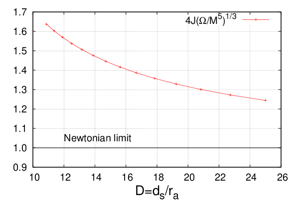
For two point particles of individual mass moving in circular orbit of radius , Kepler’s third law gives , and since the total angular momentum of the system is , we have that in Newtonian mechanics the total mass of the system , the total angular momentum , and the angular velocity satisfy
| (23) |
The deviation from the Newtonian value of the quantity on the left side of Eq. (23) can be seen in Fig. 2. The closer the black holes are, the larger the difference between the Newtonian and general relativistic prediction.
Plots of the ADM mass and the angular momentum versus the angular velocity can be seen in Fig. 3. As the black holes come together the mass and the angular momentum exhibits a minimum that signifies the innermost stable circular orbit (ISCO). As we observe from the top panel of Fig. 3 the minimum of the ADM mass is different from the minimum of the angular momentum (middle panel). The reason for this discrepancy is that the magnitude of the spin as computed by Eq. (15) is not exactly zero and therefore the sequence is not strictly speaking irrotational. This is the reason that the characteristic cusp in the mass versus angular momentum plot is absent (bottom panel). As we discussed above this issue is resolved when we iterate over so as to make the spin, Eq. (15), to be zero.


| Type | |||||||||
|---|---|---|---|---|---|---|---|---|---|
| H3 | 0.1-0.23 | 1.125 | 1.25 | 2.5 | 384 | 96 | 96 | 12 |
| 25.00 | 0.04516 | 0.98367 | -0.01633 | 0.84973 | ||||||
| 22.73 | 0.05175 | 0.98274 | -0.01726 | 0.82913 | ||||||
| 20.83 | 0.05856 | 0.98190 | -0.01810 | 0.81218 | ||||||
| 19.23 | 0.06558 | 0.98116 | -0.01884 | 0.79820 | ||||||
| 17.86 | 0.07281 | 0.98054 | -0.01946 | 0.78667 | ||||||
| 16.67 | 0.08023 | 0.98004 | -0.01996 | 0.77721 | ||||||
| 15.63 | 0.08783 | 0.97968 | -0.02032 | 0.76953 | ||||||
| 14.71 | 0.09563 | 0.97948 | -0.02052 | 0.76343 | ||||||
| 13.89 | 0.10360 | 0.97945 | -0.02055 | 0.75874 | ||||||
| 13.16 | 0.11178 | 0.97963 | -0.02037 | 0.75538 | ||||||
| 12.50 | 0.12015 | 0.98005 | -0.01995 | 0.75327 | ||||||
| 11.90 | 0.12874 | 0.98074 | -0.01926 | 0.75240 | ||||||
| 11.36 | 0.13757 | 0.98176 | -0.01824 | 0.75281 | ||||||
| 10.87 | 0.14669 | 0.98320 | -0.01680 | 0.75460 |
4 Discussion
We have successfully computed a sequence of conformally flat initial data for non-spinning equal mass BBH solutions in circular orbits. Several authors have calculated sequences of this kind as models of BBH inspiral due to the graviational wave radiation [6, 8, 9]. They used spectral methods in their computations, and produced numerical solutions in higher precision compared to ours. In the cocal code, we use standard, mostly second order, finite difference scheme. Our method is much simpler than the spectral method, and hence it is easier to extend our code to include magnetic fields or neutron stars. Also we have demonstrated that the solutions are accurate enough to reproduce the results of [6, 8, 9]. Further details of the cocal code will be discussed elsewhere.
Acknowledgements.
The authors wish to thank members of the Observatory of Meudon (LUTH) for their warm hospitality and valuable discussions. This paper is dedicated to Peter Leach on the occasion of his seventieth birthday.References
- Jackson (1975) J. D. Jackson. Classical Electrodynamics. Second Ed., John Wiley & Sons, 1975.
- Komatsu, Eriguchi, and Hachisu (1989) Hidemi Komatsu, Yoshiharu Eriguchi, and Izumi Hachisu. Rapidly rotating general relativistic stars - I. Numerical method and its application to uniformly rotating polytropes Mon. Not. R. Astron. Soc. 237, 355 (1989).
- Tsokaros and Uryū (2007) Antonios Tsokaros and Kōji Uryū. Numerical method for binary black hole/neutron star initial data Code test Phys. Rev. D 75, 044026 (2007).
- Uryū and Tsokaros (2012) Kōji Uryū and Antonios Tsokaros. New code for equilibriums and quasiequilibrium initial data of compact objects Phys. Rev. D 85, 064014 (2012).
- Gourgoulhon, Grandclément, and Bonazzola I (2002) Eric Gourgoulhon, Philippe Grandclément, and Silvano Bonazzola. Binary black holes in circular orbits. I. A global spacetime approach Phys. Rev. D 65, 044020 (2002).
- GGB II (2002) Philippe Grandclément, Eric Gourgoulhon, and Silvano Bonazzola. Binary black holes in circular orbits. II. Numerical methods and first results Phys. Rev. D 65, 044021 (2002).
- Cook and Pfeiffer (2004) Gregory B. Cook, Harald P. Pfeiffer. Excision boundary conditions for black-hole initial data. Phys. Rev. D 70, 104106 (2004).
- Caudill, Cook, Grigsby, and Pfeiffer (2004) Matthew Caudill, Gregory B. Cook, Jason D. Grigsby, and Harald P. Pfeiffer Circular orbits and spin in black-hole initial data. Phys. Rev. D 74, 064011 (2006).
- Grandclément (2010) Philippe Grandclément KADATH: A spectral solver for theoretical physics. Journal of Computational Physics 229, 9 (2010).