Optimized explicit Runge-Kutta schemes for the spectral difference method applied to wave propagation problems
Abstract
Explicit Runge–Kutta schemes with large stable step sizes are developed for integration of high order spectral difference spatial discretizations on quadrilateral grids. The new schemes permit an effective time step that is substantially larger than the maximum admissible time step of standard explicit Runge–Kutta schemes available in literature. Furthermore, they have a small principal error norm and admit a low-storage implementation. The advantages of the new schemes are demonstrated through application to the Euler equations and the linearized Euler equations.
1 Introduction
Throughout the past two decades, the development of high-order accurate spatial discretization has been one of the major fields of research in numerical analysis, computational fluid dynamics (CFD), computational aeroacoustics (CAA), computational electromagnetism (CEM) and in general computational physics characterized by linear and nonlinear wave propagation phenomena. High-order discretizations have the potential to improve the computational efficiency required to achieve a desired error level by allowing the use of coarser grids. Indeed, in modern wave propagation problems characterized by complicated geometries, complex physics and a wide disparity of length scales (e.g., large eddy simulation, turbulent combustion, flow around flapping wings, rotor-blade interaction), the need for high-accuracy solutions leads to a prohibitive computational cost when low-order (i.e., first- and second-order accurate) discretizations are used. High-order schemes have much better wave propagation properties and a truncation error that decreases more rapidly than that of low-order schemes if the solution is sufficiently smooth. Therefore, for problems that require very low numerical dissipation and small error levels, it may be advantageous to use high-order spatial discretization schemes; see for instance [8, 9, 44, 41].
Among high-order methods, the spectral difference (SD) scheme is receiving increasing attention [10, 14, 28, 31, 32, 33, 3, 29]. The SD scheme offers several interesting properties. It is able to obtain solutions with arbitrarily high order of accuracy. It can be applied to unstructured quadrilateral and hexahedral meshes (tensorial cells). The conservation laws to be solved are in differential form, avoiding the use of costly high-order accurate quadrature formulas.
Although the formulation of high-order spatial discretization is now fairly mature, the development of techniques for efficiently solving systems of ordinary differential equations (ODEs) arising from high-order accurate spatial discretizations has received less attention. The cost of solving an initial value problem up to a fixed time is inversely proportional to the time step used, so it is desirable to use the largest step size possible if the temporal discretization error is acceptable. For higher order schemes, the spectrum of the Jacobian of the semi-discretization often has increasingly large eigenvalues. As a result, the step size is often limited by stability requirements, which become stricter with higher order methods. Implicit methods allow the use of much larger step sizes, but lead to very large memory requirements that may not be feasible. Moreover, the development of efficient algebraic solvers for high-order implicit discretizations remains challenging. Thus, explicit time integration methods that allow large step sizes and require less memory seem to be an appealing alternative.
This work focuses on the development of new optimized explicit Runge-Kutta (ERK) schemes to compute wave propagation efficiently and accurately with high-order SD methods on unstructured uniform or quasi-uniform quadrilateral cell grids. The schemes are optimized with respect to the spectrum of the SD discretization, using the two-dimensional (2D) advection equation as a model problem. Linear stability optimization determines the coefficients of the stability polynomial but does not uniquely determine the full RK method. A second optimization step is used to determine the Butcher coefficients of the scheme, optimized for a small leading truncation error constant and low-storage form. The low-storage form is crucial for memory reasons, since many stages are used.
Many authors have studied the design of optimal ERK schemes with many stages for integration of high order discretizations of partial differential equations (PDEs). Past efforts focused on schemes with a relatively smaller number of stages [2, 38, 12, 30, 4]. By using the algorithm developed in [25], we are able to develop schemes with much larger number of stages and with higher order of accuracy. Our work is also the first to develop schemes specifically for the spectral difference semi-discretization. Whereas past studies have focused on application to linear problems only, and typically employed structured grids, we validate the effectiveness of our methods also on a nonlinear, fully unstructured example. Our new optimal ERK methods increase the computational efficiency of the SD method for wave propagation problems up to and , respectively for 4th-order and 5th-order accurate simulations.
The remainder of the paper is organized as follows. In Section 2, we review the SD method for tensor product cells (quadrilateral and hexahedral cells). Section 3 is devoted to the description of the two-step optimization algorithm used to design new ERK schemes, in which we first select an optimal stability polynomial and then design a corresponding ERK method. We also present the main features of the optimized methods and discuss their theoretical efficiency. Section 4 presents numerical results for three benchmark test problems, which demonstrate that the new schemes lead to large performance gains over standard ERK schemes available in the literature, for both linear and nonlinear problems. Conclusions and future directions are given in Section 5.
2 Spectral difference discretization
In this section, we review the spectral difference approach to semi-discretization of hyperbolic conservation laws.
Consider the general hyperbolic system of conservation laws over a three-dimensional domain with boundary and completed with consistent initial and boundary conditions:
| (1) |
Here, , , , , and are respectively the position vector, the vector of the conserved variables, the flux vector, source terms, and the lower and upper bound of the time interval. The spatial domain is discretized into tensor product cells with domain and boundary and .
For each cell , take a mapped coordinate system . The transformation from the standard to the physical element in the global Cartesian coordinates for the cell is given by
| (2) |
with Jacobian matrix and Jacobian determinant . The fluxes projected in the mapped coordinate system () are then related to the flux components in the global coordinate system by
| (3) |
Therefore, the hyperbolic system (1) can be written in the mapped coordinate system as
| (4) |
where and are the conserved variables and the differential operator in the mapped coordinate system, respectively.
For a -th-order accurate -dimensional scheme, solution collocation points with index are introduced at positions in each cell , with given by . Given the values at these points, a polynomial approximation of degree of the solution in cell can be constructed. This polynomial is called the solution polynomial and is usually composed of a set of Lagrangian basis polynomial of degree :
| (5) |
Therefore, the interpolation coefficients are given as where are the conserved variables at the solution points, i.e. the unknowns of the SD method.
The divergence of the mapped fluxes at the solution points is computed by introducing a set of flux collocation points with index and at positions , supporting a polynomial of degree . The evolution of the mapped flux vector in cell is then approximated by a flux polynomial , which is obtained by reconstructing the solution variables at the flux points and evaluating the fluxes at these points. The flux is represented by a separate Lagrange polynomial:
| (6) |
Hence, the coefficients of the flux interpolation are defined as
| (7) |
where is the flux vector at the cell interface. In order to maintain conservation at a cell level, the flux component normal to a face (i.e. ) must be continuous between two neighboring cells. However, the solution at a face is in general not continuous and requires the solution of a Riemann problem. For many nonlinear hyperbolic systems, such as the compressible Euler equations, the exact Riemann solution cannot be written in closed form and is prohibitively expensive to compute. Therefore, cheaper approximate Riemann solvers are typically used. The tangential component of is usually taken from the interior cell (see for instance [45]).
Taking the divergence of the flux polynomial in the solution points results in the following modified form of (4), describing the evolution of the conservative variables in the solution points:
| (8) |
where is the flux polynomial vector in the physical space whereas is the SD residual associated with . This is a system of ODEs, in time, for the unknowns .
2.1 Solution and flux points distributions
Huynh [20] showed that for quadrilateral and hexahedral cells, tensor product flux point distributions based on a one-dimensional (1D) flux point distribution consisting of the end points and the Legendre-Gauss quadrature points lead to stable schemes for arbitrary order of accuracy.
In 2008, Van den Abeele et al. [1] showed an interesting property of the SD method, namely that it is independent of the positions of its solution points in most general circumstances, for both simplex and tensor-product cells. In the above work it has been shown that the distribution of the solution points has very little influence on the properties of the SD schemes, and in fact, for linear problems, different distributions lead to identical results. This property greatly simplifies the design of SD schemes, since only the flux point distributions has to be taken care with. It also implies an important improvement in efficiency, since the solution points can be placed at flux point positions and thus a significant number of solution reconstructions can be avoided. Recently, this property has been proved by Jameson [21].
Figure 1 shows a typical distribution of flux and solution points for a third-order SD scheme in 2D.

2.2 Advection equation
The advection equation represents the simplest hyperbolic conservation law. It models the advection of a scalar conserved variable with constant advection speed . The conserved variables and the convective flux are then
| (9) | ||||
Therefore, the conservation law reads
| (10) |
2.2.1 Spectrum of the two-dimensional advection equation
Despite its simplicity, the one-dimensional advection equation is often used as a model problem to design and analyze new spatial discretization schemes for convection-dominated problems. It is also used to optimize the coefficients of time integration algorithms for CFD, and for wave propagation problems in general.
In this work, however, we use the 2D advection equation as a model. In the 2D case, the discrete operator arising from the spatial discretization is also a function of the convective velocity direction. This approach allows us to consider different wave propagation trajectories and optimize the RK coefficients by using a richer spectrum (or Fourier footprint) than that of the 1D advection equation. The richer spectrum leads to a design of more robust schemes. In the remaining part of this section, the procedure used to compute the Fourier footprint is described.
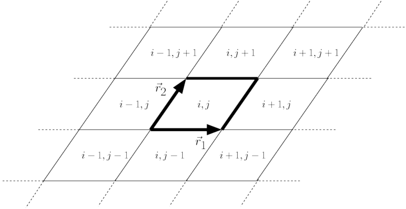
Equation (10) is discretized in space by the SD scheme. A uniform grid with periodic boundary conditions is considered. The grid is defined by a generating pattern, which is the smallest part from which the full grid can be reconstructed by periodically repeating the pattern in all directions. For the 2D case and uniform quadrilateral meshes, the generating pattern is completely defined by the vectors and (see Figure 2) whose non-dimensional form is obtained by scaling them with the length of , denoted by : and . If the dimensionless vector is chosen as , then the dimensionless mesh is completely defined by the two components of .
The advection speed in Equation (10) is defined by its amplitude and orientation angle :
| (11) |
At cell faces the solution is discontinuous, so two values for the convected variables are available. The normal flux component is calculated using the following approximate Riemann solver:
| (12) |
where is the unit normal oriented from the left to the right side and indices and indicate respectively the left and right neighboring cell to a face. In the present analysis, the internal component in each cell is used for the tangential flux component.
After the SD semi-discretization of (10) on a uniform quadrilateral mesh, the following system of ODEs is obtained:
| (13) |
where the five matrices are determined by the coefficients of the spatial discretization. They depend on the order of accuracy of the SD scheme, the generating pattern, and the advection velocity orientation angle . The column vector contains all solution point variables of the cell with indices and (Figure 2).
Inserting the following plane Fourier wave
| (14) | |||||
into Equation (13) results in
| (15) |
where is the imaginary unit number. Here, and are the wave vector and the dimensionless wave vector given by
| (16) |
and
| (17) |
where is the angle between the wave vector and the horizontal axis.
Equation (15) can be written as
| (18) |
where the matrix is defined by the SD spatial operator. The set of eigenvalues of is the spectrum or Fourier footprint of the spatial discretization. The spectrum depends on the order of accuracy of the SD scheme, the generating pattern, the direction of the convective velocity, and the dimensionless wave number vector .
Here we take a uniform Cartesian grid defined by
| (19) |
and, for a given order of accuracy, we compute the spectrum of the operator by varying , and .
3 Optimized Runge–Kutta schemes
The spectral difference semi-discretization of a PDE described in the previous section leads to an initial value problem
| (20) |
where and are the vector of the unknowns and the vector of the residuals, respectively. The number of degrees of freedom is denoted by , where is the number of cells used to discretize the domain . System (20) is typically integrated by using a high-order accurate ERK time discretization, which takes the form
| (21) | ||||
for a scalar ODE. The properties of the RK method are determined by its coefficient matrix and column vector which are referred to as the Butcher coefficients [6]. In this section, we describe our approach to designing RK schemes that maximize the absolutely stable time step size, have reasonably small error constants, and can be implemented with low storage requirements.
3.1 Optimization of the stability polynomial
Stability of RK integration is studied by applying the method (21) to the linear scalar test problem . Any RK method applied to this problem yields an iteration of the form
| (22) |
where the stability function depends only on the coefficients of the RK method ([16, Section 4.3][6, 17]):
| (23) |
Here is a column vector of size made by ones. The stability function governs the local propagation of errors, since any perturbation to the solution will be multiplied by at each subsequent step.
We say the iteration (22) is absolutely stable if
| where | (24) |
The set is referred to as the absolute stability region.
When applied to a linear system of PDEs (such as the advection or linearized Euler equations discussed in the previous section), the SD semi-discretization leads to a linear, constant-coefficient initial value problem; i.e. (20) with where is a fixed square matrix that depends on the order of accuracy of the spatial discretization, the generating pattern (see Figure 2), the direction of the convective velocity defined in Equation (11), and the dimensionless wave number vector given by Equation (17).
Application of a RK method to (20) leads to the iteration
| (25) |
where is the CFL number. Assume that is diagonalizable and let denote its eigenvalues. Then the solution is absolutely stable for CFL number if
| (26) |
Thus the maximum absolutely stable step size is
| (27) |
Although this analysis is based on the linear problem, it is often used to obtain a practical step size restriction for the nonlinear problem (20) by considering the spectrum of the Jacobian of .
In general, for an -stage, order , ERK method is a polynomial of degree that differs from the exponential function by terms of order :
| (28) |
It is natural then to design optimal polynomials by choosing the coefficients in (28) so as to maximize . The optimization problem may be stated formally as follows
Problem 1 (Stability polynomial optimization)
We solve Problem 1 using a convex optimization approach and bisection with respect to the CFL number , as described in [25]. Specifically, we fix the step size and solve the resulting convex feasibility problem, to determine whether there exists a choice of coefficients that satisfy the constraints. The upper bound for the initial bisection interval is , and we use a monomial basis. The bisection search is carried out to an accuracy of .
This approach allows us to optimize methods with large numbers of stages in order to improve the maximum absolutely stable time step . The optimization is carried out for 2nd- to 5th-order accurate schemes; the constraint points are taken as the spectrum of the SD semi-discretization of the same order of accuracy. The latter choice seems to be the most natural one. However, since in many situations the spatial error dominates and a temporal discretization should be chosen to achieve a pre-defined error tolerance at the lowest possible cost, one might think that a very stable low order ERK schemes could be a valid alternative. As shown in [34], by using a very low order of accuracy the linearly stable step size can be dramatically increased over the standard ERK schemes available in literature but such a gain reduces to about 5% over the optimal ERK methods presented in this work. Moreover, the speed-up is obtained with some relatively large sacrifices in accuracy.
Figure 3 shows the stability regions of the classical 4-stage 4th-order (ERK(4,4)) [27] and optimized 18-stage 4th-order (ERK(18,4)) methods superimposed on the Fourier footprint of the 4th-order SD methods computed varying the direction of the wave propagation velocity vector , the solution orientation defined by the angle and the dimensionless wave vector module (see Section 2.2.1). Clearly, the optimized method allows the use of a much larger step size. Notice also that the stability region of the optimized method has nearly the same shape as the convex hull of the SD spectrum.


3.2 Determination of Runge–Kutta coefficients
The choice of stability polynomial does not fully determine the method; an ERK method of stages has coefficients and only of them are constrained by the stability polynomial. We now consider the problem of finding the RK coefficients corresponding to a set of prescribed stability polynomial coefficients . We use the remaining degrees of freedom to satisfy additional nonlinear order conditions, to obtain a low-storage implementation, and ensure that the truncation error coefficients are not too large.
While the linear accuracy of the method is determined by the stability polynomial, the nonlinear accuracy depends on larger set of order conditions , where ranges from to and is simply an identifying index for the individual conditions, each of which is a polynomial of degree . For details concerning RK order conditions, see for instance [6]. We ensure that those conditions are satisfied up to order and we seek to minimize the Euclidean norm of the truncation error coefficients of order [6, 17]:
Memory requirements for RK methods are typically on the order of . To avoid the need for large amounts of memory, we employ the low-storage algorithm presented in [24], which reduces the requirement to , i.e. 3 registers per stage. The coefficients of the methods are provided in terms of the low-storage formulation, which is given in Algorithm 2. This algorithm also retains the previous solution values so that a step can be restarted if a prescribed stability or accuracy condition is not met.
The optimization problem may be stated formally as follows
Problem 2 (RK method optimization)
Here represents the conditions necessary for the method to be written in low-storage form. In practice, we impose those conditions implicitly by taking the low-storage coefficients as decision variables and computing the Butcher coefficients from them.
We use the RK-opt (”Runge–Kutta optimization”) package to search for optimized methods. This software uses MATLAB’s fmincon function with the interior-point algorithm and the multi-start global optimization toolbox. Six hundred random initial guesses were used to find each optimized RK method. The RK-opt package and its extensions [26] are freely available at https://github.com/ketch/RK-opt.
3.3 Efficiency and CFL number
Time integration with an explicit method always incurs a step size restriction based on stability. Accuracy typically also leads to a constraint on the time step, which for hyperbolic problems translates to a constraint on the CFL number, of the form , where is the largest CFL number satisfying a prescribed error tolerance. Other concerns, such as positivity, may further restrict the CFL number, but we focus on and .
If , stability is the more restrictive concern and the relative efficiency of two RK methods of order can be measured as the ratio of the maximum effective stable CFL number :
| (29) |
where denotes a safety factor applied to both schemes. If then method 1 is more efficient. This quantity measures the relative time interval integrated per unit work [23].
On the other hand, if , accuracy is the more restrictive concern so relative efficiency should be based on the ratio of step sizes, giving an equivalent global error. A first estimate, assuming that local errors simply accumulate, yields the relative efficiency measure
| (30) |
where and are the principal error norms of the two RK schemes (see Section 3.2). Note that this measure is meaningful only if both schemes have order . Although (30) is probably too simplistic because the error at each time step feeds back into the computation at the next step, it is used as a guideline for the selection of RK schemes among the optimized methods presented in this paper11 1 Notice that (30) differs from Equation in [23] by the exponent. In Kennedy et al. [23] the power of is set to because the control of the local truncation error is the main objective of the comparison [19]..
Figure 4 shows both and for 2nd- to 5th-order optimized schemes over widely used traditional explicit ERK methods of the same accuracy: the mid-point rule ERK(2,2); Heun’s 3-stage 3rd-order ERK(3,3) method [18]; the classical 4-stage 4th-order ERK(4,4) [27]; and the 6-stage 5th-order Runge–Kutta–Fehlberg ERKF(6,5) method [13]. The maximum stable CFL number defined in Section 2.2.1 is also shown for completeness.


3.4 Discussion
We provide optimized methods for , because for larger values of , the convex solvers used in the algorithm of [25] often fail due to poor numerical conditioning. However, Figures 4(a) and 4(b) already show that the marginal efficiency gain achieved by adding another stage, becomes vanishingly small for large .
Indeed, the asymptotic efficiency gain that could be achieved by using additional stages is bounded, since the classical CFL theorem implies that the scheme cannot be stable for a CFL number greater than [35]. An even tighter bound can be inferred by recalling that the stability region of an -stage ERK cannot contain the closed disk with diameter as a proper subset [22]. By determining the largest of such disks contained in the spectrum of the SD method, upper bounds on the efficiency of optimized methods can be obtained. A further refinement can be obtained by using Theorem 5 of [35], which refers to ellipses instead of only disks.
These considerations imply that, for hyperbolic PDE discretizations, only a limited number of stages are necessary to realize most of the potential efficiency gain. Based on Figure 4, it seems that the number of stages that provides a significant improvement increases with the order .
The blue lines indicate that the global error efficiency of our schemes generally decreases with the number of stages. However, for all schemes, is within of the reference scheme value. We emphasize that accuracy is not the primary concern in the design of these schemes; certainly better accuracy could be obtained if one were willing to sacrifice some stability.
Tables 1 to 4 list the value of and of the optimized schemes that are used for the test problems in the next section. Two methods have been selected for each order of accuracy. Those with fewer number of stages have an accuracy efficiency close to that of the reference methods, whereas the schemes with a large number of stages are characterized by a large value of the stability efficiency and an accuracy efficiency which is greater than . The coefficients of the selected optimized methods in terms of the low-storage formulation (see Algorithm 2 ) are listed in Appendix A.
| Method | |||||
|---|---|---|---|---|---|
| Midpoint ERK(2,2) | 2 | 1.7678 | 1.7180 | 1 | 1 |
| Optimal ERK(3,2) | 3 | 1.9587 | 7.5938 | 1.11 | 1.00 |
| Optimal ERK(8,2) | 8 | 2.0968 | 1.1294 | 1.19 | 0.98 |
| Method | |||||
|---|---|---|---|---|---|
| Heun’s ERK(3,3) | 3 | 7.5739 | 4.6296 | 1 | 1 |
| Optimal ERK(5,3) | 5 | 9.0719 | 9.9290 | 1.20 | 1.00 |
| Optimal ERK(18,3) | 17 | 1.0718 | 7.1115 | 1.42 | 0.71 |
| Method | |||||
|---|---|---|---|---|---|
| Kutta’s ERK(4,4) | 4 | 3.9534 | 1.4505 | 1 | 1 |
| Optimal ERK(9,4) | 9 | 5.6977 | 5.0640 | 1.44 | 1.03 |
| Optimal ERK(18,4) | 18 | 6.5233 | 1.1087 | 1.65 | 0.75 |
| Method | |||||
|---|---|---|---|---|---|
| Fehlberg ERK(6,5) | 6 | 2.6916 | 3.3557 | 1 | 1 |
| Optimal ERK(10,5) | 10 | 3.6164 | 5.0975 | 1.34 | 1.39 |
| Optimal ERK(20,5) | 20 | 4.2195 | 1.0490 | 1.57 | 0.95 |
The classical linear stability analysis describes the growth of truncation errors from one step to the next, but ignores the effect that roundoff and truncation errors in intermediate stages may have within a single step. Although, for conventional ERK methods, the accumulation of round-off errors during a single time step is negligible, it must be taken into account for schemes with a large number of stages. In fact, in the application of ERK schemes with many stages to time dependent PDEs, there can be a serious accumulation of errors that may even render methods unusable; this is referred to as internal instability [39, 40]. Since most of our new schemes use many stages, a thorough analysis of their internal stability properties has also been performed. All the schemes are internally stable.
4 Applications
In order to asses the efficiency and the accuracy of our new ERK schemes, we have performed a series of numerical simulations. The computations run on a machine with GHz Quad-Core Intel Xeon, using the Coolfluid 3 collaborative simulation environment [37]. Sixteen gigabytes of RAM were available. The grids have been generated using Gmsh software [15].
In Coolfluid 3, the CFL-number in two dimensions is defined as
| (31) |
with and the x- and y-components of the wave speed , and with and the width and height of a Cartesian grid cell. This definition, when applied to the Roe scheme on a structured Cartesian mesh leads to a positive and stable discretization for a CFL number smaller than unity [11]. In practical computations it has been observed that slightly larger time steps may be used without affecting stability [11].
4.1 Order verification
In this section we present the convergence study of the optimized ERK scheme listed in Tables 1 to 4. We integrate a system of nonlinear non-autonomous system of first order ODE [36, 30]
| (32) |
with the time ranging from to , and with the following initial conditions: . The analytical solution of this system is . We use the norm of the error
to study the time integration error. Here and denote the numerical solutions. Figure 5 shows the norm of the error as a function of the time step . It can be seen that for all ERK schemes the expected order of accuracy is achieved. Moreover, the new optimized methods show significantly smaller errors than the reference methods, as expected based on their smaller error constants.


4.2 Advection of a Gaussian wave in an annulus
The second problem we consider is the advection of a Gaussian wave in a 2D annulus. Such a problem models the transport of a scalar conserved variable with variable advection speed . The conserved variables and the convective flux are then
| (33) | ||||
Therefore, the conservation law reads
| (34) |
where in a 2D Cartesian space
Here is the angular velocity which is set to . Note that the ERK schemes have been optimized for the 2D advection equation with constant convective velocity (see (9)) whereas here a variable velocity is used. Therefore, the numerical results and performance presented in this section can already be used to partially asses the robustness of the new time stepping methods. All schemes were also tested using a uniform advection velocity on a uniform cartesian grid. The results of those tests are omitted since they are very similar to those of the more challenging test problem we now consider.
The initial Gaussian wave condition is centered at , and is defined as
| (35) |
where the radius is set to .
The annulus is characterized by an internal radius and an external radius . One-quarter of the annulus is discretized for the actual computations. Simulations are performed using 2nd- to 5th-order spatial and temporal discretizations from to (see Figure 6). Several CFL numbers ranging from to the maximum linearly stable one are used. A mesh with (radial direction azimuthal direction) quadrilateral cells with a maximum aspect ratio of are used for the second-order computations. Such a mesh leads to a total number of DOFs is which is held constant for higher order accurate simulations by coarsening the grid in both directions. Extrapolation boundary conditions are imposed on both circular boundaries.

The exact solution is just a clock-wise roto-translation of the initial solution and is given by (35) with , .
We solve this problem with each of the reference and optimized ERK schemes using the predicted maximum stable CFL number for each scheme. In every case, the resulting computation is stable, confirming the theoretical prediction. Figure 7 shows the maximum norm of the error vector
| (36) |
and the CPU time for each scheme. Although the number of DOF is the same in all the simulations, the error decreases rapidly with increasing order of the discretization. Remarkably, a unit increment of the order of accuracy leads to a reduction of the error of one order of magnitude and to a faster simulation (Figure 7(a)). This shows the benefit of using high-order accurate methods for wave propagation problems. As predicted, some of the highly optimized ERK schemes yield somewhat larger errors. Figure 7(b) highlights the speed-up obtained with the optimized RK schemes over the standard methods for high-order accurate simulations. Indeed, for 4th- and 5th-order computations the new schemes reduce the computational time by and , respectively. These values match very well the theoretical results shown in the previous sections.
Figure 8 shows the maximum norm error as a function of the one-step effective CFL number. Here is the exact solution at the solution point (or DOF) .
Interestingly, for some methods the error increases with increasing CFL number, while for others it actually decreases. The latter behavior is reminiscent of the behavior of many low-order schemes that are more accurate for CFL numbers close to 1 and more dissipative for small CFL numbers. In addition, we point out that a combination of a quasi uniform grid and the maximum CFL numbers obtained during the first optimization step results in stable full discretizations.


4.3 Acoustic wave propagation
In this example we solve the linearized Euler equations (LEE), which model the propagation of small perturbations in a mean flow field. They are frequently used to compute the propagation of acoustic waves in the absence of acoustic sources, e.g. turbulence production. They have been successfully used to solve in a hybrid approach for cavity flow [42], jet noise [5], and vortex–blade interaction [7].
The LEE are derived from the compressible Euler equations which mathematically describe the three physical conservation laws (i.e. conservation of mass, conservation of momentum and conservation of energy) for an inviscid fluid. Thus, the definitions of the conserved variables and the flux vector are
In these equations, is the mass density, , and are the Cartesian velocity components, is thermodynamic pressure, and is specific total energy. The velocity vector is and its magnitude is denoted by . For an ideal gas, which approximates well the thermodynamic behavior of air in a wide range of thermodynamic conditions, the specific total energy is related to the pressure and the velocity field by
| (38) |
where is the heat capacity ratio for air. Equation (38) closes the hyperbolic system (37) of five nonlinear PDEs with five unknowns.
The LEE are obtained from (37) by decomposing the primitive flow variables , and into a mean flow value and a perturbation about this mean flow :
| (39) |
Substituting these relations in (37), subtracting the mean flow terms and neglecting products of perturbations, the following sets of conserved variables and the flux components are obtained
| (40) |
| (41) |
This procedure also leads to a source term involving mean flow gradients (right-hand side of (1)):
| (42) |
which partially accounts for the refraction effects. The source term is zero in case of a uniform mean flow.
The initial solution for this numerical test has a Gaussian profile centered at the origin of the axes and it is given by
| (43) |
where the radius of the Gaussian pulse is set to . The uniform mean flow variables are , , and . Simulation are done from to . The numerical domain is a circle with radius , which is also centered at the origin of the axes. For the 2nd-order calculations, a mesh with (radial direction azimuthal direction) quadrilateral cells with a maximum aspect ratio of is used. Therefore the total number of DOFs is . As for the previous numerical test, this number is kept constant for higher order accurate simulations by coarsening the grid in both directions. Simple extrapolation boundary conditions are used. Figure 9 shows the contour plot of the acoustic pressure field at .

The exact solution for the acoustic pressure field obtained by integrating the LEE is used as a reference solution to compute the numerical error. Its analytical expression is given by (44)
| (44) |
with and the Bessel function of the first kind of order zero.
Figure 10 shows the maximum norm of the error and the CPU time for each scheme, using the predicted maximum stable CFL number. All schemes are again stable at their respective theoretical CFL values. The results are similar to those shown in Figure 7 for advection, although it appears that the spatial errors are even more dominant for this problem as the overall error is nearly the same for all time-stepping schemes of a given order.
Figure 11 shows the maximum norm of the error versus effective CFL number for a range of CFL numbers. We observe that for a fixed order of accuracy the error is almost independent of the CFL number. More precisely we find that as long as the time step is smaller than the theoretical maximum stable value, the error is dominated by the spatial discretization error. Note that a unit increment of the order of accuracy of the full discretization leads to a reduction of the error of one order of magnitude. The optimized RK schemes speed up the simulations considerably.


4.4 Vortex shedding past a wedge
This test case focuses on the von Karman vortex street past a triangular wedge [43] computed with the compressible Euler equations (37). Indeed, in the inviscid framework, vortex shedding phenomena can be described when the considered bodies present sharp corners which ensure the separation of the flow. This numerical test represents a more realistic application and it is used to study the performance of the new temporal schemes for a nonlinear system of PDEs and highly unstructured mesh. The compressible Euler equations are generally used to model the flow of an inviscid fluid, or the flow of a viscous fluid in regions where the effects of viscosity and heat conduction are negligible. Typical applications include preliminary aircraft design and rotor-flow computations.
In Figure 12 the configuration of the test case is illustrated, where the incoming flow is from left to right. The wedge is placed on the centerline of the computational domain and it is characterized by a length L. At the left boundary (the inflow) the flow is prescribed to be uniform with zero angle of attack and free-stream Mach number of . Both inlet density and inlet pressure are set to one. A pressure outlet boundary condition is imposed on the right boundary of the domain which is placed about 15 L away from the wedge. Far-field boundary conditions (i.e. uniform Dirichlet boundary conditions for the conserved variables) are imposed both on the top and bottom boundaries.

An unstructured grid with quadrilateral cells with a maximum aspect ratio of and a maximum skewness value of is used for the 2nd-order calculations. This leads to DOFs. The number of DOFs are again kept about constant for higher order accurate simulation by coarsening the grid. For this test the exact solution is not available. Therefore a reference solution is numerically computed by solving the problem on the mesh with quadrilateral cells with the 5th-order SD method ( DOFs) and the ERKF(6,5) scheme. A CFL number is used for the reference computation.
In order to avoid discontinuities near the surface of the wedge during the transitional phase that is produced by the uniform free-stream initial conditions, an intermediate solution, in which the formed vortices have not yet separated, is computed with 1st-order SD and ERK(2,2). That solution is used as the initial condition for all higher-order computations (including the reference one) which are carried out from to (see Figure 13) to generate new unsteady laminar initial solutions for each order of accuracy.

Afterwards, starting with these intermediate solutions, several computations are performed using the CFL number for each scheme and measuring the error after 0.1 seconds. Figure 14 shows the maximum norm of the error and the CPU time for each scheme. Remarkably, we observe that the new schemes, designed using linear advection on a uniform grid, perform very well for the compressible Euler equations on an unstructured grid. Indeed, they speed up the simulations considerably, while retaining a small error norm. Moreover, we highlight that the use of a quasi-uniform grid and the CFL number results in stable full discretizations. Therefore, also for this nonlinear test the theoretical stability efficiencies obtained in the first optimization step by using the 2D linear advection equation model are recovered.
5 Conclusions and future work
In this work we have developed new robust optimized explicit Runge-Kutta schemes for the spectral difference method to efficiently and accurately solve wave propagation problems on unstructured uniform or quasi-uniform non-simplex cell grids. We have shown that by using low-storage schemes with optimized stability function and reasonable leading truncation error constant, one can significantly improve the performance of the resulting method of lines discretization. By integrating high-order accurate spectral difference semi-discretizations (i.e. 3rd-, 4th- and 5th-order) with optimized Runge–Kutta methods, we have found stability efficiency improvements of to , for typical systems of hyperbolic conservation laws used in fluid dynamics. These performance gains correspond to a reduction in computational cost of to for a fixed simulation time. These improvements, which agree remarkably well with theoretical predictions based on analysis of the 2D advection equation, are obtained without significant sacrifices in accuracy. Indeed, when both spatial and temporal discretizations have the same order of accuracy the spatial error typically dominates. Therefore, for a fixed order of accuracy the error is almost independent of the CFL number and large time steps can be used.
Our results also highlight the advantage of high order schemes, which is even more pronounced when optimized time integrators are employed. The schemes designed in this work are intended for the solution of purely hyperbolic systems of conservation discretized on unstructured grids. The goal of ongoing research involves the optimization of such a family of schemes for convection-dominated problems with diffusion, where anisotropic grids are needed to discretize the domain with an economical distribution of cells.
Finally, we want to highlight that by keeping the number of degrees of freedom constant, while increasing the order of accuracy, the new schemes allow to get much more accurate solutions in about the same time, with about the same memory requirements. For example, using our optimized schemes, the proposed 5th-order discretization is actually faster than the 2nd-order discretization, when the number of degrees of freedom is held constant. Of course, the 5th-order discretization is also much more accurate. We expect that similar improvements could be obtained by using our approach to design optimized ERK schemes for other high-order accurate semi-discretizations.
Appendix A Low storage ERK coefficients
| c | |||||
|---|---|---|---|---|---|
| 0.0000000000000000 | 7.2366074728360086 | 0.0000000000000000 | 1.0000000000000000 | 0.0000000000000000 | 1.0000000000000000 |
| 7.2366074728360086 | 3.4217876502651023 | -1.2664395576322218 | 6.5427782599406470 | 0.0000000000000000 | 7.2196567116037724 |
| 5.9236433182015646 | 3.6640216242653251 | 1.1426980685848858 | -8.2869287683723744 | 0.0000000000000000 | 0.0000000000000000 |
| c | |||||
|---|---|---|---|---|---|
| 0.0000000000000000 | 9.9292229393265474 | 0.0000000000000000 | 1.0000000000000000 | 0.0000000000000000 | 1.0000000000000000 |
| 9.9292229393265474 | 5.2108385130005974 | 4.2397552118208004 | 4.4390665802303775 | 0.0000000000000000 | 2.9762522910396538 |
| 1.0732413280565014 | 3.8505327083543915 | -2.3528852074619033 | 7.5333732286056154 | 0.0000000000000000 | 3.4212961014330662 |
| 2.5057060509809409 | 7.9714199213087467 | 7.9598685017877846 | 6.5885460813015481 | 5.8415358412023582 | 5.7010739154759105 |
| 1.0496674928979783 | -8.1822460276649120 | -1.3205224623823271 | 6.3976199384289623 | 6.4219008773865116 | 4.1350769551529132 |
| -6.7488037049720317 | 8.4604310411858186 | 2.1452956294251941 | -7.3823030755143193 | 6.8770305706885126 | -1.4040672669058066 |
| -1.5868411612120166 | -1.0191166090841246 | -9.5532770501880648 | 7.0177211879534529 | 6.3729822311671305 | 2.1249567092409008 |
| 2.1138242369563969 | 6.3190236038107500 | 2.5361391125131094 | 4.0185379950224559 | -3.3679429978131387 | 0.0000000000000000 |
| c | |||||
|---|---|---|---|---|---|
| 0.0000000000000000 | 2.3002859824852059 | 0.0000000000000000 | 1.0000000000000000 | 0.0000000000000000 | 1.0000000000000000 |
| 2.3002859824852059 | 3.0214498165167158 | 2.5876919610938998 | 5.5284013909611196 | 0.0000000000000000 | 3.4076878915216791 |
| 4.0500453764839639 | 8.0256010238856679 | -1.3243708384977859 | 6.7318513326032769 | 0.0000000000000000 | 3.4143871647890728 |
| 8.9478204142351003 | 4.3621618871511753 | 5.0556648948362981 | 2.8031054965521607 | 2.7525797946334213 | 7.2292984084963252 |
| 7.2351146275625733 | 1.1292705979513513 | 5.6705507883024708 | 5.5215115815918758 | -8.9505445022148511 | 0.0000000000000000 |
| c | |||||
|---|---|---|---|---|---|
| 0.0000000000000000 | 4.9565403010221741 | 0.0000000000000000 | 1.0000000000000000 | 0.0000000000000000 | 1.0000000000000000 |
| 4.9565403010221741 | 9.7408718698159397 | 7.9377023961829174 | 3.2857861940811250 | 0.0000000000000000 | -3.7235794357769936 |
| 1.3068799001687578 | -1.7620737976801870 | -8.3475116244241754 | 1.1276843361180819 | 0.0000000000000000 | 3.3315440189685536 |
| -1.5883063460310493 | 1.4852069175460250 | -1.6706337980062214 | 1.3149447395238016 | 8.4034574578399479 | -8.2667630338402520 |
| 3.5681144740196935 | -3.3127657103714951 | 3.6410691500331427 | 5.2062891534209055 | 8.5047738439705145 | -5.4628377681035534 |
| 7.6727123317642698 | 4.8294609330498492 | 6.9178255181542780 | 8.8127462325164985 | 1.4082448501410852 | 6.0210777634642887 |
| 1.0812579255374613 | 4.9622612199980112 | 1.4887115004739182 | 4.2020606445856712 | -3.2678802469519369 | -5.7528717894031067 |
| 1.8767228084815801 | 8.7340766269850378 | 4.5336125560871188 | 7.6532635739246124 | 5.3716357620635535 | 5.0914861529202782 |
| 9.6162976936182631 | -2.8692804399085370 | -1.2705776046458739 | 4.4386734924685722 | 9.0228922115199051 | 3.8258114767897194 |
| -2.2760719867560897 | 1.2679897532256112 | 8.3749845457747696 | 6.6503093955199682 | 1.5960226946983552 | -4.6279063221185290 |
| 1.1115681606027146 | -1.0217436118953449 | 1.5709218393361746 | 1.5850209163184039 | 1.1038153140686748 | -2.0820434288562648 |
| 6.1266845427676520 | 8.4665570032598350 | -5.7768207086288348 | 1.1521721573462576 | 1.0843516423068365 | 1.4398056081552713 |
| 1.0729473245077408 | 2.8253854742588246 | -5.7340394122375393 | 1.1172750819374575 | 4.6212710442787724 | -2.8056600927348752 |
| 3.7824186468104548 | -9.2936733010804407 | -1.2050734846514470 | 7.7630223917584007 | -3.3448312125108398 | 2.2767189929551406 |
| 7.9041891347646720 | -8.4798124766803512 | -2.8100719513641002 | 1.0046657060652295 | 1.1153826567096696 | -5.8917530100546356 |
| -1.0406955693161675 | -1.6923145636158564 | 1.6142798657609492 | -1.9795868964959054 | 1.5503248734613539 | 9.1328651048418164 |
| -2.4607146824557105 | -4.7305106233879957 | -2.5801264756641613 | 1.3350583594705518 | -1.2200245424704212 | 0.0000000000000000 |
| c | |||||
|---|---|---|---|---|---|
| 0.0000000000000000 | 2.8363432481011769 | 0.0000000000000000 | 1.0000000000000000 | 0.0000000000000000 | 1.0000000000000000 |
| 2.8363432481011769 | 9.7364980747486463 | -4.6556413837561301 | 2.4992627683300688 | 0.0000000000000000 | 1.2629238731608268 |
| 5.4840742446661772 | 3.3823592364196498 | -7.7202649689034453 | 5.8668202764174726 | 0.0000000000000000 | 7.5749675232391733 |
| 3.6872298094969475 | -3.5849518935750763 | -4.0244202720632174 | 1.2051419816240785 | 7.6209857891449362 | 5.1635907196195419 |
| -6.8061183026103156 | -4.1139587569859462 | -2.1296873883702272 | 3.4747937498564541 | -1.9811817832965520 | -2.7463346616574083 |
| 3.5185265855105619 | 1.4279689871485013 | -2.4350219407769953 | 1.3213458736302766 | -6.2289587091629484 | -4.3826743572318672 |
| 1.6659419385562171 | 1.8084680519536503 | 1.9856336960249132 | 3.1196363453264964 | -3.7522475499063573 | 1.2735870231839268 |
| 9.7152778807463247 | 1.6057708856060501 | -2.8107894116913812 | 4.3514189245414447 | -3.3554373281046146 | -6.2947382217730230 |
| 9.0515694340066954 | 2.9522267863254809 | 1.6894354373677900 | 2.3596980658341213 | -4.5609629702116454 | 0.0000000000000000 |
| c | |||||
|---|---|---|---|---|---|
| 0.0000000000000000 | 1.2384169480626298 | 0.0000000000000000 | 1.0000000000000000 | 0.0000000000000000 | 1.0000000000000000 |
| 1.2384169480626298 | 1.0176262534280349 | 1.1750819811951678 | -1.2891068509748144 | 0.0000000000000000 | 3.5816500441970289 |
| 1.1574324659554065 | -6.9732026387527429 | 3.0909017892654811 | 3.5609406666728954 | 0.0000000000000000 | 5.8208024465093577 |
| 5.4372099141546926 | 3.4239356067806476 | 1.4409117788115862 | -4.0648075226104241 | 2.5583378537249163 | -2.2615285894283538 |
| 8.8394666834280744 | 1.8177707207807942 | -4.3563049445694069 | 6.0714786995207426 | 5.2676794366988289 | -2.1715466578266213 |
| -1.2212042176605774 | -6.1188746289480445 | 2.0341503014683893 | 1.0253501186236846 | -2.5648375621792202 | -4.6990441450888265 |
| 4.4125685133082082 | 7.8242308902580354 | 4.9828356971917692 | 2.4411240760769423 | 3.1932438003236391 | -2.7986911594744995 |
| 3.8039092095473748 | -3.7642864750532951 | 3.5307737157745489 | -1.2813606970134104 | -3.1106815010852862 | 9.8513926355272197 |
| 5.4591107347528367 | -4.5078383666690258 | -7.9318790975894626 | 8.1625711892373898 | 4.7631196164025996 | -1.1899324232814899 |
| 4.8731855535356028 | -7.5734228201432585 | 8.9120513355345166 | 1.0171269354643386 | -9.8853727938895783 | 4.2821073124370562 |
| -2.3007964303896034 | -2.7149222760935121 | 5.7091009196320974 | 1.9379378662711269 | 1.9274726276883622 | -8.2196355299900403 |
| -1.8907656662915873 | 1.1833684341657344 | 1.6912188575015419 | 7.4408643544851782 | 3.2389860855971508 | 5.8113997057675074 |
| 8.1059805668623763 | 2.8858319979308041 | 1.0077912519329719 | -1.2591764563430008 | 7.5923980038397509 | -6.1283024325436919 |
| 7.7080875997868803 | 4.6005267586974657 | -6.8532953752099512 | 1.1996463179654226 | 2.0635456088664017 | 5.6800136190634054 |
| 1.1712158507200179 | 1.8014887068775631 | 1.0488165551884063 | 4.5772068865370406 | -8.9741032556032857 | -3.3874970570335106 |
| 1.2755351018003545 | -1.5508175395461857 | 8.3647761371829943 | 8.3622292077033844 | 2.6899932505676190 | -7.3071238125137772 |
| 8.0422507946168564 | -4.0095737929274988 | 1.3087909830445710 | -1.4179124272450148 | 4.1882069379552307 | 8.3936016960374532 |
| 9.7508680250761848 | 1.4949678367038011 | 9.0419681700177323 | 1.3661459065331649 | 6.2016148912381761 | 0.0000000000000000 |
| c | |||||
|---|---|---|---|---|---|
| 0.0000000000000000 | 2.5978835757039448 | 0.0000000000000000 | 1.0000000000000000 | 0.0000000000000000 | 1.0000000000000000 |
| 2.5978835757039448 | 1.7770088002098183 | 4.0436600785287713 | 6.8714670697294733 | 0.0000000000000000 | -1.3317784091400336 |
| 9.9045731158085557 | 2.4816366373161344 | -8.5034274641295027 | 1.0930247604585732 | 0.0000000000000000 | 8.2604227852898304 |
| 2.1555118823045644 | 7.9417368275785671 | -6.9508941671218478 | 3.2259753823377983 | -2.3934051593398129 | 1.5137004305165804 |
| 5.0079500784155040 | 3.8853912968701337 | 9.2387652252320684 | 1.0411537008416110 | -1.9028544220991284 | -1.3058100631721905 |
| 5.5922519148547800 | 1.4550516642704694 | -2.5631780399589106 | 1.2928214888638039 | -2.8200422105835639 | 3.0366787893355149 |
| 5.4499869734044426 | 1.5875173794655811 | 2.5457448699988827 | 7.3914627692888835 | -1.8326984641282289 | -1.4494582670831953 |
| 7.6152246625852738 | 1.6506056315937651 | 3.1258317336761454 | 1.2391292570651462 | -2.1990945108072310 | 3.8343138733685103 |
| 8.4270620830633836 | 2.1180932999328042 | -7.0071148003175443 | 1.8427534793568445 | -4.0824306603783045 | 4.1222939718018692 |
| 9.1522098071770008 | 1.5593923403495016 | 4.8396209710057070 | 5.7127889427161162 | -1.3776697911236280 | 0.0000000000000000 |
| c | |||||
|---|---|---|---|---|---|
| 0.0000000000000000 | 1.7342385375780556 | 0.0000000000000000 | 1.0000000000000000 | 0.0000000000000000 | 1.0000000000000000 |
| 1.7342385375780556 | 2.8569004728564801 | -1.1682479703229380 | 8.8952052154583572 | 0.0000000000000000 | 1.4375468781258596 |
| 3.0484982420032158 | 6.8727044379779589 | -2.5112155037089772 | 8.8988129100385194 | 0.0000000000000000 | 1.5081653637261594 |
| 5.5271395645729193 | 1.2812121060977319 | -5.5259960154735988 | 3.5701564494677057 | 1.9595487007932735 | -1.4575347066062688 |
| 4.7079204549750037 | 4.9137180740403122 | 2.9243033509511740 | 2.4232462479216824 | -6.9871675039100595 | 3.1495761082838158 |
| 1.5652540451324129 | 4.7033584446956857 | -4.7948973385386493 | 1.2727083024258155 | 1.0592231169810050 | 3.5505919368536931 |
| 1.8602224049074517 | 4.4539998128170821 | -5.3095533497183016 | 1.1126977210342681 | 1.0730426871909635 | 2.3616389374566960 |
| 2.8426620035751449 | 1.2259824887343720 | -2.3624194456630736 | 5.1360709645409097 | 8.9257826744389124 | 1.0267488547302055 |
| 9.5094727548792268 | 2.0616463985024421 | 2.0068995756589547 | 1.1181089682044856 | -1.4078912484894415 | 3.5991243524519438 |
| 6.8046501070096010 | 1.5941162575324802 | -1.4985808661597710 | 2.7881272382085232 | -2.6869890558434262 | 1.5172890003890782 |
| 5.9705366562360063 | 1.2953803678226099 | 4.8941228502377687 | 4.9032886260666715 | -6.5175753568318007 | 1.8171662741779953 |
| 1.8970821645077285 | 1.7287352967302603 | -1.0387512755259576 | 4.1871051065897870 | 4.9177812903108553 | 2.8762263521436831 |
| 2.9742664004529606 | 1.1660483420536467 | -1.3287664273288191 | 4.4602463796686219 | 4.6017684776493678 | 4.6350154228218754 |
| 6.0813463700134940 | 7.7997036621815521 | 7.5858678822837511 | 1.4897271251154750 | -6.4689512947008251 | 1.5573122110727220 |
| 7.3080004188477765 | 3.2563250234418012 | -4.3321586294096939 | 2.6244269699436817 | 4.4034728024115377 | 2.0001066778080254 |
| 9.1656999044951792 | 1.0611520488333197 | 4.8199700138402146 | -4.7486056986590294 | 6.1086885767527943 | 9.1690694855534305 |
| 1.4309687554614530 | 6.5891625628040993 | -7.0924756614960671 | 2.3219312682036197 | 5.0546454457410162 | 2.0474618401365854 |
| 4.1043824968249148 | 8.3534647700054046 | -8.8422252029506054 | 6.2852588972458059 | 5.4668509293072887 | -3.2336329115436924 |
| 8.4898255952298962 | 9.8972579458252483 | -8.9129367099545231 | 5.4473719351268962 | 7.1414182420995431 | 3.2899060754742177 |
| 3.3543896258348421 | 4.3010116145097040 | 1.5297157134040762 | 2.4345446089014514 | -1.0558095282893749 | 0.0000000000000000 |
References
- [1] K. Abeele, C. Lacor, and Z. J. Wang, On the stability and accuracy of the spectral difference method, Journal of Scientific Computing, 37 (2008), pp. 162–188.
- [2] V. Allampalli, R. Hixon, M. Nallasamy, and S. D. Sawyer, High-accuracy large-step explicit Runge-–Kutta (HALE-RK) schemes for computational aeroacoustics, Journal of Computational Physics, 228 (2009), pp. 3837–3850.
- [3] Balan, A. and May, G. and Schöerl, J., A stable high-order spectral difference method for hyperbolic conservation laws on triangular elements, Journal of Computational Physics, 231 (2012), pp. 2359 – 2375.
- [4] M. Bernardini and S. Pirozzoli, A general strategy for the optimization of Runge–Kutta schemes for wave propagation phenomena, Journal of Computational Physics, 228 (2009), pp. 4182–4199.
- [5] C. Bogey, C. Bailly, and D. Juvé, Computation of flow noise using source terms in linearized Euler’s equations, AIAA Journal, 40 (2002), pp. 235–243.
- [6] J. C. Butcher, Numerical methods for ordinary differential equations, John Wiley & Sons, Ltd, Chichester, UK, Mar. 2008.
- [7] G. Chen and S. S. Collis, Multimodel methods for optimal control of aeroacoustics, in AIAA Paper, Reno, Nevada, U.S.A., 2005, pp. 1–10.
- [8] M.-H. Chen, B. Cockburn, and F. Reitich, High-order RKDG methods for computational electromagnetics, Journal of Scientific Computing, 22-23 (2005), pp. 205–226.
- [9] T. Colonius and S. K. Lele, Computational aeroacoustics: progress on nonlinear problems of sound generation, Progress in Aerospace Sciences, 40 (2004), pp. 345–416.
- [10] C. Cox, C. Liang, and M. Plesniak, Spectral difference solution of incompressible flow over an inline tube bundle with oscillating cylinder, in ASME 2012 Pressure Vessels and Piping Conference, Toronto, Ontario, Canada, 2012, pp. 1–12.
- [11] H. Deconinck, Numerical methods for flow calculation in turbomachines – Introduction to artificial dissipation and shock capturing high resolution upwind schemes for the Euler equations, von Karman Institute Lecture Series, (1996), pp. 1–38.
- [12] R. Diehl, K. Busch, and J. Niegemann, Comparison of Low-Storage Runge-Kutta Schemes for Discontinuous Galerkin Time-Domain Simulations of Maxwell’s Equations, Journal of Computational and Theoretical Nanoscience, 7 (2010), pp. 1572–1580.
- [13] E. Fehlberg, Low-order classical Runge-Kutta formulas with stepsize control and their application to some heat transfer, tech. report, NASA TR R-315, National Aeronautics and Space Administration, Marshall Space Flight Center, Marshall, AL, 1969.
- [14] J. Gao, Z. Yang, and X. Li, An optimized spectral difference scheme for CAA problems, Journal of Computational Physics, 231 (2012), pp. 4848–4866.
- [15] C. Geuzaine and J.-F. Remacle, Gmsh: A 3-D finite element mesh generator with built-in pre- and post-processing facilities, International Journal for Numerical Methods in Engineering, 79 (2009), pp. 1309–1331.
- [16] S. Gottlieb, D. I. Ketcheson, and C.-W. Shu, Strong stability preserving Runge-Kutta and multistep time discretizations, World Scientific Publishing Company, 2011.
- [17] E. Hairer and G. Wanner, Solving ordinary differential equations II: stiff and differential-algebraic problems, Springer-Verlag, 14 (1991).
- [18] K. Heun, Neue Methoden zur approximativen integration der differentialgleichungen ener unabläingigen Veränderliehen, Zeitschrift für Angewandte Mathematik und Physik, 45 (1900), pp. 23–28.
- [19] M. E. Hosea and L. F. Shampine, Efficiency comparisons of methods for integrating ODEs, Computers & Mathematics with Applications, 28 (1994), pp. 45–55.
- [20] H. T. Huynh, A flux reconstruction approach to high-order schemes including discontinuous Galerkin methods, in 18th AIAA Computational Fluid Dynamics Conference, no. June, Miami, Florida, U.S.A., 2007, pp. 1–42.
- [21] A. Jameson, A proof of the stability of the spectral difference method for all orders of accuracy, Journal of Scientific Computing, 45 (2010), pp. 348–358.
- [22] R. Jeltsch and O. Nevanlinna, Largest disk of stability of explicit Runge-Kutta methods, BIT Numerical Mathematics, 18 (1978), pp. 500–502.
- [23] C. A. Kennedy, M. H. Carpenter, and R. M. Lewis, Low-storage, explicit Runge-Kutta schemes for the compressible Navier-Stokes equations, Applied Numerical Mathematics, 35 (2000), pp. 177–219.
- [24] D. I. Ketcheson, Runge–-Kutta methods with minimum storage implementations, Journal of Computational Physics, 229 (2010), pp. 1763–1773.
- [25] D. I. Ketcheson and A. J. Ahmadia, Optimal Runge–Kutta stability regions. http://arxiv.org/abs/1201.3035, July 2012.
- [26] D. I. Ketcheson and M. Parsani, RK-opt user manual, tech. report, 2012.
- [27] W. Kutta, Beitrag zur näherungsweisen integration totaler differentialgleichungen, Zeitschrift für Angewandte Mathematik und Physik, 46 (1901), pp. 435–453.
- [28] C. Liang, J. Chen, and J. D. Lee, Spectral difference solution of two-dimensional unsteady compressible micropolar equations on moving and deformable grids, in 50th AIAA Aerospace Sciences Meeting including the New Horizons Forum and Aerospace Exposition, Nashville, Tennessee, U.S.A., 2102, pp. 1–12.
- [29] Lodato, G. and Castonguay, P. and Jameson, A., Discrete filter operators for large-eddy simulation using high-order spectral difference methods, International Journal for Numerical Methods in Fluids, (2012).
- [30] J. Niegemann, R. Diehl, and K. Busch, Efficient low-storage Runge-Kutta schemes with optimized stability regions, Journal of Computational Physics, 231 (2011), pp. 372–364.
- [31] K. Ou and A. Jameson, Towards computational flapping wing aerodynamics of realistic configurations using spectral difference method, in 20th AIAA Computational Fluid Dynamics Conference, Honolulu, Hawaii, U.S.A., 2011, pp. 1–17.
- [32] M. Parsani, G. Ghorbaniasl, and C. Lacor, Validation and application of an high-order spectral difference method for flow induced noise simulation, Journal of Computational Acoustics, 19 (2011), pp. 241–268.
- [33] M. Parsani, G. Ghorbaniasl, C. Lacor, and E. Turkel, An implicit high-order spectral difference approach for large eddy simulation, Journal of Computational Physics, 229 (2010), pp. 5373–5393.
- [34] M. Parsani, D. I. Ketcheson, and W. Deconinck, Optimized low-order explicit Runge–Kutta schemes for the high-order spectral difference method, in 11th Finnish Mechanics Days, Oulu, Finland, 2012, pp. 1–6.
- [35] J. M. Sanz-Serna and M. N. Spijker, Regions of stability, equivalence theorems and the Courant-Friedrichs-Lewy condition, Numerische Mathematik, 49 (1986), pp. 319–329.
- [36] D. Stanescu and W. G. Habashi, 2N-storage low dissipation and dispersion Runge-Kutta schemes for computational acoustics, Journal of Computational Physics, 143 (1998), pp. 674–681.
- [37] Coolfluid 3 Team, Coolfluid 3. http://coolfluid.github.com/, 2012.
- [38] T. Toulorge and W. Desmet, Optimal Runge-Kutta Schemes for discontinuous Galerkin space discretizations applied to wave propagation problems, Journal of Computational Physics, (2011).
- [39] J. G. Verwer, Explicit Runge-Kutta methods for parabolic partial differential equations, Applied Numerical Mathematics, 22 (1996), pp. 359–379.
- [40] J. G. Verwer, W. H. Hundsdorfer, and B. P. Sommeijer, Convergence Properties of the Runge-Kutta-Chebyshev Method, in Numerische Mathematik, vol. 178, 1990, pp. 157–178.
- [41] P. E. Vincent and A. Jameson, Facilitating the adoption of unstructured high-order methods amongst a wider community of fluid dynamicists, Mathematical Modelling of Natural Phenomena, 6 (2011), pp. 97–140.
- [42] C. Wagner, T. Hüttl, and P. Sagaut, eds., Large-eddy simulation for acoustics, Cambridge University Press, cambridge ed., 2007.
- [43] L. Wang and D. J. Mavriplis, Implicit solution of the unsteady Euler equations for high-order accurate discontinuous Galerkin discretizations, Journal of Computational Physics, 225 (2007), pp. 1994–2015.
- [44] Z. J. Wang, High-order methods for the Euler and Navier–Stokes equations on unstructured grids, Progress in Aerospace Sciences, 43 (2007), pp. 1–41.
- [45] Z. J. Wang, Y. Liu, G. May, and A. Jameson, Spectral difference method for unstructured grids II: extension to the Euler equations, Journal of Scientific Computing, 32 (2006), pp. 45–71.