To be concrete, we first concentrate on a simplest interacting quantum field theory with a conserved axial current; namely, a linear sigma model which contains a Dirac fermion interacting with a scalar field.

$$S=\int\!dt\,d^{3}x\,\left[i\bar{\psi}\gamma^{\mu}D_{\mu}\psi-D_{\mu}\phi^{*}D^{\mu}\phi-m^{2}\phi^{*}\phi-\lambda(\phi^{*}\phi)^{2}-g\left(\bar{\psi}\frac{1+\gamma^{5}}{2}\psi\phi^{*}+\bar{\psi}\frac{1-\gamma^{5}}{2}\psi\phi\right)\right.\\ \left.-\frac{1}{2}h_{\mu\nu}T^{\mu\nu}+{\mathcal{O}}(h^{2})\right],$$

(2)

with

	$\displaystyle D_{\mu}\psi=$	$\displaystyle(\partial_{\mu}-i\gamma^{5}A_{\mu})\psi,$
	$\displaystyle D_{\mu}\phi=$	$\displaystyle(\partial_{\mu}-2iA_{\mu})\phi,$
	$\displaystyle T^{\mu\nu}=$	$\displaystyle\frac{i}{4}\bar{\psi}\gamma^{\mu}(\stackrel{{\scriptstyle\rightarrow}}{{D^{\nu}}}-\stackrel{{\scriptstyle\leftarrow}}{{D^{\nu}}})\psi+\mu\leftrightarrow\nu+\textrm{scalar contributions}.$		(3)

We have include in the action the coupling to external axial U(1) gauge field $A_{\mu}$ and small metric perturbation $h_{\mu\nu}$.

The symmetries associated with the background fields are anomalous, and the anomalies are captured by the Ward identities:

	$\displaystyle\partial_{\mu}J^{\mu}_{5}=$	$\displaystyle-\frac{1}{48\pi^{2}}\epsilon^{\mu\nu\rho\sigma}F_{\mu\nu}F_{\rho\sigma},$		(4)
	$\displaystyle\partial_{\mu}T^{\mu\nu}=$	$\displaystyle F^{\nu\rho}\big(J_{\rho}-\frac{1}{12\pi^{2}}{\epsilon_{\rho}}^{\sigma\alpha\beta}A_{\sigma}F_{\alpha\beta}\big),$		(5)

where $J^{\mu}_{5}=\bar{\psi}\gamma^{\mu}\gamma^{5}\psi$, $F_{\mu\nu}$ is the field strength associated with $A_{\mu}$. We note that the axial current is conserved in the absence of sources.

The goal here is to calculate the chiral vortical coefficient at zero chemical potential ($A_{0}=0$). As explained in Refs. [9], this coefficient is not a proper kinetic coefficient, but is basically an equilibrium quantity given by the behavior of the retarded two-point Green’s function between the current $J_{A}^{i}$ and the momentum density $T^{0j}$ at zero frequency and small momenta,

$$G_{R}^{i,0j}(\omega,k)\Big|_{\omega=0}=i\epsilon_{ijn}k_{n}\sigma_{A}^{\mathcal{V}}+O(k^{2})$$

(6)

The fact that we are interested in the zero-frequency limit allows the chiral vortical coefficient to be related to an Euclidean Green’s function

$$iG_{R}^{i,0j}=\mathcal{G}^{i,0j}=\frac{\delta}{\delta A_{i}}\frac{\delta}{\delta g_{oj}}Z=\langle J_{A}^{i}T^{0j}\rangle+\text{contact terms},$$

(7)

where $\mathcal{G}^{i,0j}$ is the Euclidean (Matsubara) Green’s function. At zero frequency we can take our source fields $A_{\mu}$ and $h_{\mu\nu}$ to be time independent from the start. With this configuration, it is easy to see that the right hand side of the anomalous Ward identities in equations (5) vanish and the symmetry is effectively restored.

We will demonstrate diagramatically, using an argument similar to that of Coleman and Hill who showed the non-normalization of the Chern-Simons term obtained by integrating out massive fermions in 3D¹¹ 1 It is known that there are caveats to the Coleman-Hill theorem (see for example [14]). Namely when there are parity-violating interactions in the initial Lagrangian. However, as there are no such terms, they do not concern the treatment in this paper., that only diagrams that are present in the zero-coupling limit give non-zero contributions to the CVE coefficient[15]. The calculation at zero coupling is given in [8], and our argument would show that the calculation is exact at any value of the coupling constant.

Let us now look at a generic diagram at non-zero coupling (see figure 1(a)). All such diagrams can be obtained from the $n$-scalar effective vertices with exactly one insertion of $J^{\mu}_{5}$ and $T_{\mu\nu}$ by contracting external scalar potentials and integrating over the scalar momenta. Let us look at the central block of the construction:

$$\Gamma^{(n)}_{ij}(p,q,\kappa_{1},\cdots,\kappa_{n}).$$

(8)

Graphically, this is a one-loop graph with $n$ external dynamical scalars, 1 external graviton $b_{i}$ and 1 external source gauge boson $a_{i}$ (figure 1(b)).

The gauge invariance of the time independent source fields implies:

	$\displaystyle p^{i}\Gamma^{(n)}_{ij}(p,q,\kappa_{1},\cdots,\kappa_{n})=0,$
	$\displaystyle q^{j}\Gamma^{(n)}_{ij}(p,q,\kappa_{1},\cdots,\kappa_{n})=0.$		(9)

Differentiating these equations with respect to $p^{r}$ and $q^{r}$ and then letting $p$ and $q$ be zero respectively we get:

$\displaystyle\begin{aligned} \Gamma^{(n)}_{ijk_{1}\cdots k_{n}}(0,q,\kappa_{1},\cdots,\kappa_{n})=0\\ \Gamma^{(n)}_{ijk_{1}\cdots k_{n}}(p,0,\kappa_{1},\cdots,\kappa_{n})=0\end{aligned}\;\;\Rightarrow\begin{aligned} \Gamma^{(n)}_{ijk_{1}\cdots k_{n}}(p,q,\kappa_{1},\cdots,\kappa_{n})={\mathcal{O}}(p)\\ \Gamma^{(n)}_{ijk_{1}\cdots k_{n}}(p,k,\kappa_{1},\cdots,\kappa_{n})={\mathcal{O}}(k),\end{aligned}$

(10)

where we have used the fact that these functions are analytic in $k$. For $n=0$ the two momenta $p$ and $q$ are not independent and hence we derive:

$\displaystyle\Gamma^{(0)}_{ijk_{1}\cdots k_{n}}(p,-p)={\mathcal{O}}(p).$

(11)

However, for $n>0$ these two momenta are independent and (10) implies:

$\displaystyle\Gamma^{(n)}_{ijk_{1}\cdots k_{n}}(p,q,\kappa_{1},\cdots,\kappa_{n})={\mathcal{O}}(pq).$

(12)

This is all we need for our proof. The full contribution to the CVE coefficient is the sum of the zero coupling diagram calculated above and diagrams with internal scalars. The latter can be constructed from our effective $n$ point vertices by contracting the external scalar lines.

Two cases arise. If the source fields $a_{i}$ and $b_{i}$ are attached to the same fermion loop, the total diagram is ${\mathcal{O}}(k^{2})$ by equation (12). Using the same argument, if they are attached to two different fermion loops, we again get that the total diagram is ${\mathcal{O}}(k^{2})$ by applying equation (10) for each loop. The same reasoning can be applied to the case with the scalar stress tensor insertion and the case with scalar internal loops, implying that all such diagrams are ${\mathcal{O}}(k^{2})$. On the other hand the chiral vortical coefficient is the term linear in the external momentum of the two-point Green’s function. Thus, only the one-loop free diagram can contribute to the CVE. This completes the proof.

It is important to note that the analyticity arguments given above require the mass of the scalars to be non-zero. Given the fact that scalars generically acquire mass at finite temperature, this requirement is equivalent to the statment that we are not sitting at a second order phase transition.

We now turn to the case with fermions coupled to dynamical gauge fields. As claimed in the introduction, in this case, the CVE in fact does receive corrections. We show that for the non-abelian theory at leading order in $1/N$ there is a single class of diagrams that give non-zero contributions to the CVE coefficient. To demonstrate this, we point out where the arguments of the previous section are affected. The action is:

$$S=\int dt\,d^{3}x\,\big(i\bar{\psi}\cancel{D}\psi-\frac{1}{4g^{2}}V_{\mu\nu}V^{\mu\nu}+eA_{\mu}J^{\mu}_{5}-\frac{1}{2}h_{\mu\nu}T^{\mu\nu}+{\mathcal{O}}(h^{2})\big),$$

(13)

where $D$ and $V_{\mu\nu}$ are respectively the covariant (vector-like) coupling and curvature tensor associated with the dynamical gauge field $V_{\mu}$. We assume one flavor of fermions and we suppress the Lie group indices.

Following the steps of the scalar-coupling case discussed above, we come across two issues and we tackle them one by one, one of which ultimately leads to radiative corrections. The first difference is that there are now potentially gapless excitations associated with the gluons. The infrared singularities associated with such massless modes threaten to ruin the analyticity arguments that were crucial in the proof. This is the same caveat that also came up in the original Coleman and Hill paper[15]. However, since we are working with non-abelian theories, the solution provided there does not apply.

Fortunately, non-abelian theories at finite temperature do produce a mass gap non-perturbatively [16]. To take advantage of this fact, we divide the arguments of the previous section into two steps. First, we perturbatively integrate out the fermionic fields to give effective vertices with gauge fields, the axial source and the graviton (respectively $V_{\mu}$, $A_{i}$ and $h_{0i}$) as external lines. According to the previous section, the diagrams with more than two external legs are ${\mathcal{O}}(k^{2})$.

Next, we evaluate the expectation value of these effective vertices non-perturbatively. This method allows us to use both our perturbative diagramatic arguments of the previous section while steering clear of the IR singularities that plague perturbative analysis of gauge fields.

The second difference is that the anomaly (equation (5)) no longer vanishes in the absence of external sources and is now given by:

$$\partial_{\mu}J^{\mu}_{5}=-\frac{g^{2}C(r)}{16\pi^{2}\sqrt{-g}}\epsilon^{\mu\nu\rho\sigma}V_{\mu\nu}V_{\rho\sigma}+\cdots,$$

(14)

where we have ommited the terms higher order in the external sources. This is a big problem as the arguments of the previous section all depended on the conservation of the axial current.

At this point, we split the diagrams into two groups depending on the form of the Energy-Momentum tensor (see figure 2). The first group has a fermionic Energy Momentum insertion (figure 2(a)) and the second has the gauge part (figure 2(b)). For the first group, at leading order in $1/N$, we have a single fermion loop to which both the axial current $J^{i}_{5}$ and the energy-momentum tensor $T^{0i}$ are attached. The anomalous contribution of such one loop diagrams is exactly captured in equation (14). Expanding the right hand side in metric perturbations, we see that to linear order, the anomaly only depends on the trace of the perturbation and thus does not contribute to correlators involving a single insertion of $T^{0i}$.

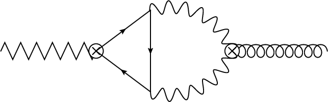
However, it turns out that there are certain diagrams in the second class that do in fact contribute to the CVE. Since in the absence of the anomaly in equation (14), there would be no radiative corrections, it is clear that the only contributing diagram are those that include a triangle subdiagram as in figure 3(a). Figure 3(b) shows the leading order diagram in this class which we now proceed to calculate.

Since we already know that the only contribution comes from the anomaly in (14), we can replace the triangle part of the two loop diagram with the effective vertex:

$$J^{\mu}_{\text{Anom}}=-\frac{g^{2}C(r)}{4\pi^{2}\sqrt{-g}}\epsilon^{\mu\nu\rho\sigma}V_{\nu}\partial_{\rho}V_{\sigma}$$

(15)

which captures the divergence of the axial current, and we are effectively left with only a one loop diagram (figure 3(c)). The calculation of the diagram is slightly complicated by the fact that different components of the gauge field receive different effective masses which are in general very important for our arguments. However, in this case it turns out that there are no infrared divergences even at zero effective mass and we present the calculation with this simplification.

The anomalous contribution to the Euclidean Green’s function is:

$$\mathcal{G}^{i,0j}_{\text{Anom}}=\langle J^{i}_{\text{Anom}}T^{0j}\rangle=\frac{-g^{2}TC(r)d(G)}{4\pi^{2}}\epsilon^{ijm}k_{m}\sum\hskip-15.0pt\int\frac{d^{3}p}{(2\pi)^{3}}\frac{\omega^{2}-\frac{p^{2}}{3}}{(\omega^{2}+p^{2})^{2}}+\cdots$$

(16)

where $d(G)$ is the dimension of the adjoint representation and we have expanded up to first order in $k$. It is now a simple matter to carry out the sum and the integral:

$$\mathcal{G}^{i,0j}_{\text{Anom}}=\frac{-g^{2}C(r)d(G)}{48\pi^{4}}\epsilon^{ijm}k_{m}\int dp\,p\frac{1-e^{-2\frac{p}{T}}-4e^{\frac{-p}{T}}\frac{p}{T}}{\left(1-e^{\frac{-p}{T}}\right)^{2}}\to\frac{g^{2}C(r)d(G)}{48\pi^{4}}\epsilon^{ijm}k_{m},$$

(17)

where in the last step we have removed the divergent zero temperature contribution before doing the integral. In fact, at zero temperature, this contribution is not allowed by full Lorentz symmetry and vanishes (This is also verified by direct calculation). Therefore, any regulator that respects full Lorentz symmetry in the zero temperature limit would reproduce the same result.

We now read off the leading order correction to the CVE coefficient in the large N limit:

$$\sigma^{\mathcal{V}}_{\small Correction}=\frac{g^{2}C(r)d(G)}{48\pi^{2}}T^{2}.$$

(18)

In order to see the connection between the 3-dimensional Chern-Simons term and the CVE, we dimensionally reduce the theory on the compactified time direction[5]. To this end, we rename the relevant sources:

	$\displaystyle a_{i}$	$\displaystyle=A_{i}(x),$		(19)
	$\displaystyle b_{i}$	$\displaystyle=Tg_{0i},$		(20)

which transform under gauge and coordinate transformations with respective parameters $\alpha$ and $\epsilon_{\mu}$ as follows:

	$\displaystyle a_{i}$	$\displaystyle\to a_{i}+\partial_{i}\alpha,$		(21)
	$\displaystyle b_{i}$	$\displaystyle\to b_{i}+T\left(\nabla_{i}\epsilon_{0}+\nabla_{0}\epsilon_{i}\right),$		(22)

where $\epsilon_{\mu}$ is the diffeomorphism parameter ($x^{\mu}\to x^{\mu}+\epsilon^{\mu}$). As we argued in section 2, these 3-dimensional gauge transformations are not anomalous, even in the presence of anomalies in the underlying 4-dimensional theory²² 2 For coupling to gauge fields, this is only true at leading order in $1/N$.. The term of concern in the effective action is:

$$S_{eff}=i\,\kappa\int{d^{3}x\epsilon_{ijk}}a_{i}\partial_{j}b_{k}=i\,\kappa T\int{d^{4}x\epsilon_{ijk}}a_{i}\partial_{j}b_{k},$$

(23)

where in the final equality we have inserted a spurious factor of $T$ along with a trivial time integral in order to make contact with the 4-dimensional 2 point function at hand. With this definition, the Green’s function becomes:

$$\mathcal{G}^{i,0j}=T^{2}\frac{\delta}{\delta a_{i}}\frac{\delta}{\delta b_{j}}Z_{eff}=-\kappa T^{2}\epsilon_{ijk}p_{k},$$

(24)

which leads to a contribution ot the CVE coefficient of

$$\sigma^{\mathcal{V}}_{A}=\kappa T^{2}.$$

(25)

To see the quantization of the coefficient $\kappa$, we put the system on a 3 torus of sides $L_{1}$, $L_{2}$ and $L_{3}$. The periodicity of the manifold dictates the periodicty of the compact gauge fields $a_{i}$ and $b_{i}$. Using large gauge transformations $\alpha=\dfrac{2\pi}{e}\dfrac{x_{i}}{L_{i}}$ and $\epsilon_{0}=\dfrac{2}{T}\dfrac{x_{i}}{L_{i}}$, we see:

	$\displaystyle a_{i}$	$\displaystyle\equiv a_{i}+\frac{2\pi}{eL_{i}},$		(26)
	$\displaystyle b_{i}$	$\displaystyle\equiv b_{i}+\frac{2}{L_{i}},$		(27)

where $e$ is the electric charge and the factor 2 in the time translation parameter $\epsilon_{0}$ is compensating for the anti-periodicity of fermions in the time direction.

We then perform a large gauge transformation on the $a_{i}$ fields with $\alpha=2\pi n\dfrac{x_{3}}{eL_{3}}$, with $n\in\mathds{Z}$. The change in the action is:

$$\delta S_{eff}=2\pi ni\frac{\kappa}{e}\int\limits_{x_{3}=0}\!\epsilon_{3jk}\partial_{j}b_{k}.$$

(28)

Choosing a field configuration with non-trivial winding around the compact directions such as $b_{2}=\dfrac{2x_{1}}{L_{1}L_{2}}$, the variation becomes:

$$\delta S_{eff}=2\pi ni\frac{\kappa}{e}\int\limits_{x_{3}=0}\!\epsilon_{312}\partial_{1}b_{2}=4\pi ni\frac{\kappa}{e},$$

(29)

which gives us the desired quantization result of $\kappa\in\dfrac{e}{2}\mathds{Z}$.³³ 3 This is half the expected result of integer $\kappa$ values and is solely due to the fact that the fermions are anti-periodic in the thermal direction as stated under equation (27).

We now look at the Kaluza-Klein reduction of the action (2) at zero coupling. The fermions decompose on the thermal circle with periodicity $\beta=\frac{1}{T}$ as:

$\displaystyle\psi(t,x)=e^{2\pi in\frac{t}{T}}\psi_{n}(x),\;\;n\in\mathds{Z}+\frac{1}{2},$

(30)

and we assume the background sources have no time dependence. At zero coupling the different Matsubara frequencies do not mix and we can analyze the partition function mode by mode. For the $n$’th mode we have:

$$S=\frac{1}{T}\int d^{3}x\,\big(i\bar{\psi}_{-n}\cancel{\partial}\psi_{n}+A_{\mu}J_{5,n}^{\mu}-h_{0i}T_{n}^{0i}\big),$$

(31)

with

	$\displaystyle J_{5,n}^{\mu}=$	$\displaystyle\bar{\psi}_{-n}\gamma^{\mu}\gamma^{5}\psi_{n},$
	$\displaystyle T^{0i}_{n}=$	$\displaystyle\frac{i}{4}\bar{\psi}_{-n}\gamma^{0}(\stackrel{{\scriptstyle\rightarrow}}{{\partial^{i}}}-\stackrel{{\scriptstyle\leftarrow}}{{\partial^{i}}})\psi_{n}-n\pi\bar{\psi}_{-n}\gamma^{i}\psi_{n}.$		(32)

The diagram to be evaluated is given in figure 1(a) with no internal vertices. We have:

$\displaystyle\mathcal{G}^{i,0j}=-T\int\frac{d^{3}p}{(2\pi)^{3}}\text{Tr}\frac{\cancel{(p+k)}_{3}-2\pi mT\gamma^{0}}{(p+k)^{2}+4\pi^{2}m^{2}T^{2}}\left(\frac{\gamma^{0}}{4T}(2p+k)^{j}-m\pi\gamma^{j}\right)\frac{\cancel{p}_{3}-2\pi mT\gamma^{0}}{p^{2}+4\pi^{2}m^{2}T^{2}}\gamma^{i}\gamma^{5},$

(33)

where $\cancel{p}_{3}$ denotes contraction with $\gamma^{i}$, the spatial gamma matrices. We have:

$\displaystyle\epsilon_{ijn}\mathcal{G}^{i,0j}=$

$\displaystyle-T\int\frac{d^{3}p}{(2\pi)^{3}}\frac{\epsilon_{ijn}\text{Tr}(\gamma^{0}\gamma^{r}\gamma^{s}\gamma^{i}\gamma^{5})N_{rs}^{j}}{((p+k)^{2}+4\pi^{2}m^{2}T^{2})(p^{2}+4\pi^{2}m^{2}T^{2})},$

(34)

where

	$\displaystyle N_{rs}^{j}=$	$\displaystyle(-2\pi mT)(-\pi m\delta^{j}_{r})p_{s}-(p+k)_{r}\frac{1}{4T}(2p+k)^{j}p_{s}+(p+k)_{r}(-\pi m\delta^{j}_{s})(-2\pi mT)$
	$\displaystyle=$	$\displaystyle-2\pi^{2}m^{2}T\delta^{j}_{r}k_{s}-\frac{1}{4T}k_{r}p_{s}(2p+k)^{j}+\text{ Sym in }r\leftrightarrow s.$		(35)

Using the above and taking the limit of $k\to 0$, we have:

$\displaystyle\lim_{k\to 0}\epsilon_{ijn}\mathcal{G}^{i,0j}=$

$\displaystyle T\int\frac{d^{3}p}{(2\pi)^{3}}\frac{\epsilon_{ijn}4\epsilon^{rsi}(2\pi^{2}m^{2}T\delta^{j}_{r}k_{s}+\frac{1}{2T}k_{r}p_{s}p^{j})}{(p^{2}+4\pi^{2}m^{2}T^{2})^{2}}.$

(36)

This integral is of course divergent and needs to be regularized. Here we simply use the relation between different integrals in dimensional regularization⁴⁴ 4 Here we just need the simplest of these relations: $$\int\frac{d^{d}l}{(2\pi)^{d}}\frac{l^{\mu}l^{\nu}}{(l^{2}+\Delta)^{2}}=\frac{-\Delta}{d-2}\int\frac{d^{d}l}{(2\pi)^{d}}\frac{1}{(l^{2}+\Delta)^{2}}.$$ . Pauli-Villars regularization gives the same result:

	$\displaystyle\lim_{k\to 0}\epsilon_{ijn}\mathcal{G}^{i,0j}=$	$\displaystyle 16m^{2}T^{2}k_{n}\int\limits_{0}^{\infty}dp\frac{p^{2}}{(p^{2}+4\pi^{2}m^{2}T^{2})^{2}},$
	$\displaystyle=$	$\displaystyle 2\big|m\big|Tk_{n}.$		(37)

And finally we write down the contribution to the CVE coefficient for each mode:

$$\sigma^{\mathcal{V}}_{A,m}=\big|m\big|T.$$

(38)

Which satisfies the quantization condition in the previous section. We evaluate the full CVE coefficient:

$$\sigma_{A}^{\mathcal{V}}=T\sum\limits_{m=-\infty}^{\infty}\sigma_{A,m}^{\mathcal{V}}=2T^{2}\sum\limits_{m=\frac{1}{2}}^{\infty}m\to\frac{1}{12}T^{2}.$$

(39)

Where we have used the $\zeta$-function regularization. This is the same result as [8]. In essence, this calculation is the same with the order of the 3-dimensional momentum integral and the Matsubara sum.

This work is supported, in part, by DOE grant DE-FG02-00ER41132. The authors thank David B. Kaplan and Larry Yaffe for discussion. We are also greatful to Hai-cang Ren for pointing out an error in the first version of this paper.

References

- [1] S. Bhattacharyya, S. Lahiri, R. Loganayagam, and S. Minwalla, “Large rotating AdS black holes from fluid mechanics,” JHEP 0809 (2008) 054, arXiv:0708.1770 [hep-th].
- [2] J. Erdmenger, M. Haack, M. Kaminski, and A. Yarom, “Fluid dynamics of R-charged black holes,” JHEP 0901 (2009) 055, arXiv:0809.2488 [hep-th].
- [3] N. Banerjee, J. Bhattacharya, S. Bhattacharyya, S. Dutta, R. Loganayagam, et al., “Hydrodynamics from charged black branes,” JHEP 1101 (2011) 094, arXiv:0809.2596 [hep-th].
- [4] D. T. Son and P. Surowka, “Hydrodynamics with Triangle Anomalies,” Phys.Rev.Lett. 103 (2009) 191601, arXiv:0906.5044 [hep-th].
- [5] N. Banerjee, J. Bhattacharya, S. Bhattacharyya, S. Jain, S. Minwalla, et al., “Constraints on Fluid Dynamics from Equilibrium Partition Functions,” arXiv:1203.3544 [hep-th].
- [6] K. Jensen, “Triangle Anomalies, Thermodynamics, and Hydrodynamics,” arXiv:1203.3599 [hep-th]. 4+epsilon pages, REVTeX 4.1/ v2: updated references.
- [7] Y. Neiman and Y. Oz, “Relativistic Hydrodynamics with General Anomalous Charges,” JHEP 1103 (2011) 023, arXiv:1011.5107 [hep-th].
- [8] K. Landsteiner, E. Megias, and F. Pena-Benitez, “Gravitational Anomaly and Transport,” Phys.Rev.Lett. 107 (2011) 021601, arXiv:1103.5006 [hep-ph].
- [9] K. Landsteiner, E. Megias, and F. Pena-Benitez, “Anomalies and Transport Coefficients: The Chiral Gravito-Magnetic Effect,” arXiv:1110.3615 [hep-ph].
- [10] J.-H. Gao, Z.-T. Liang, S. Pu, Q. Wang, and X.-N. Wang, “Chiral Anomaly and Local Polarization Effect from Quantum Kinetic Approach,” arXiv:1203.0725 [hep-ph].
- [11] V. P. Nair, R. Ray, and S. Roy, “Fluids, anomalies, and the chiral magnetic effect: A group-theoretic formulation,”Phys. Rev. D 86 (Jul, 2012) 025012.
- [12] R. L. K. Jensen and A. Yarom, “Hydrodymanics with Gravitational Anomalies from Thermodynamics on Cones,”. To appear.
- [13] H. L. y. De-fu Houya and H. cang Ren, “A Possible Higher Order Correction to the Vortical Conductivity in a QED Plasma,”. To appear.
- [14] A. Khare, R. MacKenzie, and M. B. Paranjape, “On the Coleman-Hill theorem,” Phys.Lett. B343 (1995) 239–243, arXiv:hep-th/9408091 [hep-th].
- [15] S. Coleman and B. Hill, “No more corrections to the topological mass term in qed3,” Physics Letters B 159 (1985) no. 23, 184 – 188.
- [16] D. J. Gross, R. D. Pisarski, and L. G. Yaffe, “Qcd and instantons at finite temperature,”Rev. Mod. Phys. 53 (Jan, 1981) 43–80.
- [17] E. Witten, “Global Aspects of Current Algebra,” Nucl.Phys. B223 (1983) 422–432.
- [18] E. Witten, “Global Gravitational Anomalies,” Commun.Math.Phys. 100 (1985) 197.