Functional renormalisation group for few-nucleon systems:
SU(4) symmetry and its breaking

Michael C. Birse, Boris Krippa, Niels R. Walet Affiliation: Theoretical Physics Division, School of Physics and Astronomy, University of Manchester, Manchester, M13 9PL, UK

August 24, 2026

Abstract

We apply the functional renormalisation group to few-nucleon systems. Our starting point is a local effective action that includes three- and four-nucleon interactions, expressed in terms of nucleon and two-nucleon boson fields. The evolution of the coupling constants in this action is described by a renormalisation group flow. We derive these flow equations both in the limit of exact Wigner SU(4) symmetry and in the realistic case of broken symmetry. In the symmetric limit we find that the renormalisation flow equations decouple, and can be combined into two sets, one of which matches the known results for bosons, and the other result matches the one for a single flavour of spin $1/2$ fermions. The equations show universal features in the unitary limit, which is obtained when the two-body scattering length tends to infinity. We calculate the spin-quartet neutron-deuteron scattering length and the deuteron-deuteron scattering lengths in the spin-singlet and quintet channels.

Keywords:

Deuteron-deuteron scattering, nucleon-deuteron scattering, functional renormalisation group, SU(4) symmetry, Wigner supermultiplet

pacs

21.45.-v, 24.10.Eq, 25.45.-z, 11.10.Hi

I Introduction

Few-body physics provides a solid starting point for analysing various nonperturbative approaches and methods which can then be used for studying more complicated many-body problems. The study of few-body systems also allows us to determine the input parameters needed for those complex problems, without the need to rely on further approximations. One promising method is the Functional Renormalisation Group (FRG) [1, 2], as it provides a framework that can simultaneously describe both few- and many-body systems. Some reviews of the method and its applications can be found in Refs. [3, 4, 5].

The approach is based on a running effective action (REA) which is a generalisation of the standard quantum mechanical effective action – the generating functional of the one-particle irreducible Green functions. The REA includes the effects of all the fluctuations with momenta in the region $q^{2}\gtrsim k^{2}$ where $k$ is a running scale. This is achieved by introducing a regulator that, either sharply or smoothly, suppresses the contribution of modes with $q^{2}\lesssim k^{2}$ . The FRG describes the evolution of this action as the cut-off scale $k$ is lowered. As $k$ approaches zero, all fluctuations are included and thus the full effective action is recovered.

The FRG method has already been applied to few-body problems in a number of papers [6, 7, 8, 9, 10]. In Ref. [6], it was exploited to derive the Skornyakov–Ter-Martirosyan equation for three-body systems [11]. The Efimov effect [12] in bosonic and fermionic systems was addressed in Ref. [7]. An important extension of the approach was developed in Ref. [8] to treat the four-body problem in the presence of the three-body Efimov effect, and the process of dimer-dimer scattering was studied in detail in Ref. [10]. This shows one of the key strengths of the FRG method, which is its universality. With relatively minor changes it can be adopted to study a large variety of problems in particle, nuclear and condensed matter physics. Some representative examples can be found in Refs. [13, 14, 15].

Up to now, most applications of the FRG have been to particle physics and condensed matter systems. In the present work we apply it to systems of up to four nucleons, laying the groundwork for extensions to larger numbers of nucleons and to nuclear matter. One important aspect of our implementation of the FRG is the introduction of bosonic fields to describe interacting pairs of nucleons. This will be very useful for future work since it will allow us to link the scattering of nucleons in vacuum to pairing in systems of many nucleons, as in Ref. [13]. This study of few-nucleon systems allows us to develop some of the tools and determine the parameters that will be needed in such work. In this context, it is helpful to make use of Wigner’s SU(4) “supermultiplet” symmetry, which is known to be a very good approximate symmetry for light nuclei [16], and even for some two-nucleon processes, provided the momenta involved are large compared with the inverse scattering lengths [17].

The effective action is the Legendre transform of the logarithm of the partition function, $\Gamma[\phi_{c}]=W[J]-J\cdot\phi_{c}$ , where $e^{W}$ is the partition function in the presence of an external source $J$ [18]. The functional $\Gamma$ is the generator of the one-particle-irreducible Green’s functions, and it reduces to the usual effective potential for homogeneous systems. One of the reasons to work with $\Gamma$ rather than $W$ is that we can introduce a renormalisation group flow to determine $\Gamma$ [1]. A running version of the effective action is defined by introducing an artificial gap in the energy spectrum for the fields which depends on a momentum scale $k$ . Thus we define a different effective action for each $k$ by integrating over components of the fields with momenta $q>k$ only. The RG trajectory then interpolates between the classical action of the underlying field theory (at large $k$ ), and the full effective action (at zero $k$ ) [20]. The intermediate actions along the trajectory are not physically meaningful.

The flow equation for the effective action is a functional differential equation of the form

\partial_{k}\Gamma=-\frac{i}{2}\,\STr\left[(\partial_{k}R)\,(\Gamma^{(2)}-R)^{-1}\right].

(1)

where $\Gamma^{(2)}$ denotes the second functional derivative taken with respect to the fields entering the action, and $R$ is a matrix of cut-off functions. These functions act as regulators, suppressing the contributions of fluctuations with momenta below the running scale $k$ , and thus driving the evolution of the system as $k$ is lowered. The structure of the evolution equation is rather straightforward, the main complexity is in the operation $\STr$ , which is the supertrace, which is taken over both energy-momentum variables and internal indices. It is needed since we consider a mixed system of fermions (nucleons) and bosonic dimers in this work.

The main advantage of this version of the RG is that the right-hand-side of Eq. (1) involves a single integral over energy and momentum. It thus has the form of a one-loop integral, where $(\Gamma^{(2)}-R)^{-1}$ can be thought of as the matrix of single-particle propagators dressed by all fluctuations above the scale $k$ . Since Eq. (1) is exact and therefore nonperturbative,questions of diagrammatic expansion do not arise in this framework, in contrast to other versions of the RG and many traditional approaches to many-body physics. Nonetheless, despite its simple structure, this equation describes the running of a complicated object – $\Gamma$ is in general a non-local functional of all the fields describing our system.

Since exact solution of a functional differential equation is usually not possible, in practical applications, the REA is usually truncated to a finite number of local terms. The choice of these is guided by the relevant physics in the system we wish to describe, and by insights from effective field theories. This truncation reduces the full functional differential equation (1) to a set of coupled ODE’s for the running coupling constants and renormalisation factors multiplying those terms in the action. These equations are straightforward to solve nonperturbatively using standard methods. It is the choice of the physics we want to describe that determines the form of the expansion of the REA.

The use of local interactions means that the FRG method has close links to approaches based on effective field theories [22, 23]. In some cases, for example the action used to study the Efimov effect in three-boson systems, the terms included are just the leading terms of the corresponding effective field theory. In other cases, such as the applications to dense matter, strict power counting arguments cannot be used and we must rely on the need to describe emergent aspects of the physics that are known to be important, such as superfluidity.

In the limit where $k$ is much larger that all the physical scales in our system, $k$ becomes the only important scale. The effects of the physical scales, for example the scattering lengths, become negligible in this regime and the evolution equations then show scaling behaviour with $k$ . This behaviour is governed by the unitary limit, where the inverse two-body scattering lengths vanish. In this limit, all of the evolution equations collapse to simple universal forms for large enough values of the cut-off scale $k$ . Moreover, since all the inverse scattering lengths are negligible, these equations have SU(4)-symmetric forms. These universal equations can then be used to obtain boundary conditions for the evolution equations away from the unitary limit. We present the detailed form of these equations in the Appendix, where we show that they form two decoupled sets of equations.

The set of equations that describes three or four particles in spatially symmetric states displays the Efimov effect [12]. In these channels, scale invariance is broken by the appearance of an infinite tower of three-body bound states, with subsequent energies in a constant ratio. A single three-body initial condition needs to be specified to fix the energies of all these states.

In the main body of the paper we derive a general set of equations for the evolution of the REA, without assuming SU(4) symmetry. Nonetheless, this symmetry plays a pivotal role in our approach. As just mentioned, the initial conditions are imposed at a scale where SU(4) is a very good symmetry. Initially the evolution remains in this regime, and it is only when it reaches scales $k\sim 1/a$ that SU(4)-breaking effects can become large. In the two body sector, the symmetry is lost in the physical limit ( $k\rightarrow 0$ ) for quantities like the scattering lengths themselves. Perhaps surprisingly, SU(4) remains a good approximate symmetry for three- and four-body scattering at threshold. Working with the same combinations of couplings that decouple in the SU(4) limit, we find that the mixing remains small, except in narrow regions of the three-body parameter that controls the positions of the Efimov states.

One of these sets describes the channels where the nucleons are in states of mixed spatial symmetry and it has the same form as that for a system of fermions with spin degrees of freedom only, as derived in Ref. [10]. The other set describes the spatially symmetric channels and, after a suitable redefinition of coupling constants, it matches the evolution equations for a system of interacting bosons in Ref. [7]. Despite the similar forms of the two sets of equations, the differences in their numerical coefficients have profound physical consequences. In particular, the equations for spatially symmetric systems leads to the Efimov effect [12] and limit-cycle behaviour of the 3-body couplings [24]. In contrast these effects do not occur for few-fermion systems without spatial symmetry.

In the next section we set out the form of the REA we use in our applications of the FRG to few-nucleon systems, and in Sec. III we obtain the evolution equations for the running parameters in that action. Then, in Section IV, we apply these to analyse scattering in three- and four-nucleon systems for realistic $NN$ scattering lengths. We compare our results to those in the SU(4) limit, details of which can be found in Appendix A. Finally, some technical details of the link between scattering lengths and REA are discussed in Appendix B.

II Running effective action

Since our ultimate goal is to study pairing in dense nuclear matter, we must isolate the relevant degrees of freedom. As is well known, the nuclear force is just strong enough to generate a bound state, the deuteron, in one of the $S$ -wave channels. Its isospin-1 analogue is only just unbound and appears as a virtual state very close to threshold. We thus find it useful to introduce boson fields to describe the lowest two-body states in both these channels. If one imagines starting from an effective action with a local two-body interaction between the fermions, the boson fields can be introduced using a Hubbard-Stratonovitch transformation, which is exact in this case. We use the notation $\boldsymbol{t}$ for the (spin-triplet) vector-isoscalar boson field, corresponding to the deuteron, and $\boldsymbol{s}$ for the (spin-singlet) scalar-isovector one. These we refer to collectively as “dimers”, and label by a capital $D$ . We reserve the lower-case label $d$ for a deuteron, and $N$ for a generic nucleon. Finally, when specifying quantum numbers of particular channels, we use the $SO(4)$ notation $(S,I)$ , where $S$ and $I$ denote the resultant spin and isospin quantum numbers, respectively. In the present work, we assume that isospin is a good symmetry. The use of such dibaryon fields was first suggested in Ref. [25] in the context of effective field theories.

The key approximation we make is to truncate the full REA to one with only a finite number of parameters, so that the functional differential equation can be replaced by a set of ordinary differential equations. No further approximations are made, which means that the solution of the resulting equations is nonperturbative in all their couplings. In the present case, we introduce a set of local contact interactions in the channels of interest, as well as kinetic terms for the dimer fields. In principle we could also have added effective ranges for the interactions using the forms used in effective field theory; in this first application we have not included such effects. The form for the REA we use is

$\displaystyle\Gamma$	$\displaystyle=$	$\displaystyle\int d^{4}p\,\psi_{m_{t}m_{s}}^{\dagger}(p_{0},\boldsymbol{p})\left(p_{0}-\frac{p^{2}}{2M}+i\epsilon\right)\psi_{m_{t}m_{s}}(p_{0},\boldsymbol{p})$	(2)
		$\displaystyle+\int d^{4}p\,t_{i}^{\dagger}(p_{0},\boldsymbol{p})\left(Z_{\phi,t}p_{0}-Z_{m,t}\frac{p^{2}}{4M}-u_{1,t}+i\epsilon\right)t_{i}(p_{0},\boldsymbol{p})$
		$\displaystyle+\int d^{4}p\,s_{a}^{\dagger}(p_{0},\boldsymbol{p})\left(Z_{\phi,s}p_{0}-Z_{m,s}\frac{p^{2}}{4M}-u_{1,s}+i\epsilon\right)s_{a}(p_{0},\boldsymbol{p})$
		$\displaystyle+\Gamma_{2}+\Gamma_{3}+\Gamma_{4}.$

Since the action at the start of the evolution is obtained by bosonising a purely fermionic one, the boson fields should be non-propagating auxiliary fields for $k\rightarrow\infty$ . Their wave function and kinetic-mass renormalisation factors ( $Z_{\phi,i}$ and $Z_{m,i}$ ) should tend to zero in this limit. When we run the action as we lower the cut-off scale $k$ , these fields become dynamical, and the renormalisation factors grow.

The bosonisation introduces self-energies for the boson fields ( $u_{1,i}$ ) and couplings of the dimers to pairs of nucleons in the $(1,0)$ and $(0,1)$ two-body channels. These couplings are described by the term,

$\displaystyle\Gamma_{2}$	$\displaystyle=$	$\displaystyle\int\delta^{(4)}(p_{1}+p_{2}-p_{3})d^{4}p_{1}d^{4}p_{2}d^{4}p_{3}\mathcal{V}_{2}$	(3)
$\displaystyle\mathcal{V}_{2}$	$\displaystyle=$	$\displaystyle\frac{1}{2\sqrt{2}}g_{t}\left[\boldsymbol{t}^{\dagger}(p_{30},\boldsymbol{p}_{3})\cdot\left[\psi(p_{10},\boldsymbol{p}_{1})\psi^{C}(p_{20},\boldsymbol{p}_{2})\right]^{(1,0)}+\text{h.c.}\right]$	(4)
		$\displaystyle+\frac{1}{2\sqrt{2}}g_{s}\left[\boldsymbol{s}^{\dagger}(p_{30},\boldsymbol{p}_{3})\cdot\left[\psi(p_{10},\boldsymbol{p}_{1})\psi^{C}(p_{20},\boldsymbol{p}_{2})\right]^{(0,1)}+\text{h.c.}\right],$	(4)

where

\psi_{m_{t_{2}}m_{s_{2}}}^{C}=\tau_{m_{s_{1}}m_{s_{2}}}^{2}\sigma_{m_{t_{1}}m_{t_{2}}}^{2}\psi_{m_{t_{1}}m_{s_{1}}}.

(5)

Since $\boldsymbol{t}^{\dagger}$ is a $(1,0)$ tensor and $\boldsymbol{s}^{\dagger}$ a $(0,1)$ one, the scalar products in Eq. (4) should be understood as being taken in either spin or isospin space, as appropriate. The values of the coupling constants $g_{i}$ depend on a choice of scale in the dimer fields when they are introduced by the Hubbard-Stratonovitch transformation. Thus we must find that the values of the $g_{i}$ do not appear separately in physical quantities, but only in combinations such as $g_{i}^{2}/u_{1,i}$ . An illustration of this is provided by the discussion of the evolution of the $u_{1,i}$ in the next section. The unobservable coupling constants $g_{i}$ do not run in vacuum and, for simplicity, we choose their values to be equal,

g_{t,s}=g.

(6)

To describe the three-nucleon channels, we introduce a set of local dimer-nucleon interactions, described by the term

$\displaystyle\Gamma_{3}$	$\displaystyle=$	$\displaystyle-\int\delta^{(4)}(p_{1}+p_{3}-p_{2}-p_{4})d^{4}p_{1}d^{4}p_{2}d^{4}p_{3}d^{4}p_{4}\mathcal{V}_{3,DN}$	(7)
$\displaystyle\mathcal{V}_{3,DN}$	$\displaystyle=$	$\displaystyle\sum_{i,j=t,s}\lambda^{(1/2,1/2)}_{ij}\left[i^{\dagger}(p_{30},\boldsymbol{p}_{3})\psi^{\dagger}(p_{10},\boldsymbol{p}_{1})\right]^{(1/2,1/2)}\cdot\left[\psi(p_{20},\boldsymbol{p}_{2})j(p_{40},\boldsymbol{p}_{4})\right]^{(1/2,1/2)}$	(8)
		$\displaystyle\quad+\lambda^{(3/2,1/2)}_{tt}\left[t^{\dagger}(p_{30},\boldsymbol{p}_{3})\psi^{\dagger}(p_{10},\boldsymbol{p}_{1})\right]^{(3/2,1/2)}\cdot\left[\psi(p_{20},\boldsymbol{p}_{2})t(p_{40},\boldsymbol{p}_{4})\right]^{(3/2,1/2)}$
		$\displaystyle\quad+\lambda^{(1/2,3/2)}_{ss}\left[s^{\dagger}(p_{30},\boldsymbol{p}_{3})\psi^{\dagger}(p_{10},\boldsymbol{p}_{1})\right]^{(1/2,3/2)}\cdot\left[\psi(p_{20},\boldsymbol{p}_{2})s(p_{40},\boldsymbol{p}_{4})\right]^{(1/2,3/2)},$

where $\lambda^{(1/2,1/2)}_{ts}=\lambda^{(1/2,1/2)}_{st}$ . These have been expressed in terms of interactions in the doublet-doublet channel, with spin-isospin quantum numbers $(1/2,1/2)$ , and the quartet-doublet channels, with quantum numbers $(3/2,1/2)$ or $(1/2,3/2)$ . The $(1/2,1/2)$ channel has the quantum numbers of the ground states of ³H and ³He.

Finally, we introduce one class of four-nucleon interactions, represented by local two-body dimer-dimer interactions and described by the term

$\displaystyle\Gamma_{2,DD}$	$\displaystyle=$	$\displaystyle-\int\delta^{(4)}(p_{1}+p_{3}-p_{2}-p_{4})d^{4}p_{1}d^{4}p_{2}d^{4}p_{3}d^{4}p_{4}\mathcal{V}_{2,DD},$	(9)
$\displaystyle\mathcal{V}_{2,DD}$	$\displaystyle=$	$\displaystyle\frac{1}{2}\sum_{i=t,s}u_{2,i}\biggl(\boldsymbol{i}^{\dagger}(p_{10},\boldsymbol{p}_{1})\cdot\boldsymbol{i}(p_{20},\boldsymbol{p}_{2})\,\boldsymbol{i}^{\dagger}(p_{30},\boldsymbol{p}_{3})\cdot\boldsymbol{i}(p_{40},\boldsymbol{p}_{4})$	(10)
		$\displaystyle\qquad-\frac{1}{3}\boldsymbol{i}^{\dagger}(p_{10},\boldsymbol{p}_{1})\cdot\boldsymbol{i}^{\dagger}(p_{30},\boldsymbol{p}_{3})\,\boldsymbol{i}(p_{20},\boldsymbol{p}_{2})\cdot\boldsymbol{i}(p_{40},\boldsymbol{p}_{4})\biggr)$
		$\displaystyle+u_{2,ts}\biggl(\boldsymbol{t}^{\dagger}(p_{10},\boldsymbol{p}_{1})\cdot\boldsymbol{t}(p_{20},\boldsymbol{p}_{2})\,\boldsymbol{s}^{\dagger}(p_{30},\boldsymbol{p}_{3})\cdot\boldsymbol{s}(p_{40},\boldsymbol{p}_{4})\biggr)$
		$\displaystyle+\frac{1}{12}\sum_{ij=t,s}\bar{u}{}_{2,ij}\boldsymbol{i}^{\dagger}(p_{10},\boldsymbol{p}_{1})\cdot\boldsymbol{i}^{\dagger}(p_{30},\boldsymbol{p}_{3})\,\boldsymbol{j}(p_{20},\boldsymbol{p}_{2})\cdot\boldsymbol{j}(p_{40},\boldsymbol{p}_{4}),$

where $\bar{u}{}_{2,ts}=\bar{u}{}_{2,st}$ . The $u_{2,i}$ terms act in the $(2,0)$ and $(0,2)$ two-dimer (four-nucleon) channels, the $u_{2,ts}$ terms act in the $(1,1)$ channel, and the $\bar{u}_{2}$ terms act in the $(0,0)$ channel. Only the last of these has the quantum numbers of the ground state of the $\alpha$ particle.

The behaviour for large $k$ is particularly simple. In this region, the regulator provides the only scale and every coupling varies as a power of $k$ . The effects of SU(4)-breaking also become negligible here and so the evolution equations reduce to the simpler, SU(4)-symmetric forms discussed in Appendix A. This allows us to determine the initial conditions on the evolution here and these then provide the physical input into our approach.

Most of the parameters are “irrelevant” in the technical sense that the low-energy results from our action in the physical limit ( $k\rightarrow 0$ ) do not depend strongly on the precise values of the initial conditions imposed at very large $k$ . However, there are three exceptions and these provide the physical input into our approach. Two of them are the self-energies, $u_{1,i}$ , which are “relevant” parameters in RG language, as discussed in Ref. [27]. Their values at $k=0$ determine the strength of the interaction between the fermions and can be related either to the $NN$ scattering lengths, $a_{t}$ and $a_{s}$ , or, in the channel with the bound state, to the deuteron binding energy,

\mathcal{E}_{d}=-\frac{1}{Ma_{t}^{2}}.

(11)

The third parameter is associated with the spatially-symmetric channel of the three-nucleon system. This is the channel that displays the Efimov effect [12] and as a result the evolution of its coupling constant for it has a limit-cycle behaviour at large- $k$ . Just as in the analogous EFT treatment [24], one piece of three-body data is needed to fix the starting point on this cycle. Here we choose the nucleon-deuteron scattering length in the spin-doublet channel, and explore how four-nucleon observables are related to it.

III Evolution equations

To derive the evolution equations for the coupling constants in our action, we substitute the parametrisation given in the previous section into the right-hand side of Eq. (1). The inverse of the second derivative of $\Gamma$ forms a scale-dependent propagator, and the driving terms for the coupling constants all have structure of one-loop integrals, with differing numbers of external fields. In general these include expressions with powers of fields or derivatives beyond those contained in our truncated action. We therefore need to expand the loop integrals in powers of the fields and non-localities (i.e., in energies and momenta) and pick out those terms that match the structures listed in the previous section. The scale-dependent coefficient in front of each structure then gives us the driving term in the differential equation for the corresponding coupling constant.

As well as the choice of truncation, we also need to make a choice of the point around which we expand our energies. Since we concentrate on the physics at the dimer threshold, we choose our expansion points for this state; other choices are possible, but suffer from numerical complications arising from linking the flows both above and below threshold. For the dimers, we choose the energy of the lowest two-body bound state, $\mathcal{E}_{d}$ . In the four-nucleon sector, for example, this means that we expand around the deuteron-deuteron threshold. For the nucleons we expand around one half of this binding energy. Thus in the nuclear-dimer channels of the the three-nucleon system we expand about an energy $\mathcal{E}_{d}/2$ below the the scattering threshold. This procedure can be justified rigorously in the limit of exact SU(4) symmetry, as discussed further below, but it is only approximate in the general case. It could thus lead to a slower convergence than expected of the expansion.

Finally, we need to choose the forms for the cut-off functions in the regulators for the nucleons and dimers. Here we take the form suggested by Litim [26] for both, as it is well-suited for partially analytic calculations. It is also optimised for actions truncated to purely local (energy-independent) interactions, as also discussed in more detail by Pawlowski [5]. The regulators are thus given by

	$\displaystyle R_{N}(q;k)$	$\displaystyle=\frac{k^{2}-q^{2}}{2M}\theta(k-q),$		(12)
	$\displaystyle R_{D}(q;k)$	$\displaystyle=Z_{\phi}(k)\frac{k^{2}-q^{2}}{4M}\theta(k-q).$		(13)

Note that we have assumed that the two $Z_{\phi}$ ’s are equal; this can be shown to hold in the expansion scheme we use here, see Eq. (23) below. The inclusion of the wave-function renormalisation factor in the definition of $R_{D}$ has the advantage of allowing us to scale out the parameters $g$ , $M$ and $a_{t}$ , leaving much simpler, dimensionless expressions. For example, a generic three-body coupling $\lambda$ has a natural scaling of the form

\Lambda(\kappa)=\frac{1}{a_{t}^{2}Mg^{2}}\lambda(k).

(14)

Analogously a generic four-body coupling $u_{2}$ can be scaled as

U_{2}(\kappa)=g^{-4}M^{-3}a_{t}^{-3}u_{2}(k).

(15)

III.1 One-boson terms

The evolution equations for $u_{1,i}$ , $Z_{\phi,i}$ and $Z_{m,i}$ are relatively straightforward in vacuum. Their forms are the same as in the simpler case studied in Ref. [10]; For example, both the $u_{1,i}$ satisfy the differential equation

\partial_{k}u_{1,i}(k)=\frac{g^{2}}{2}\frac{1}{\left(2\pi\right)^{3}}\int d^{3}q\frac{\partial_{k}R_{{N}}(q;k)}{\left(\frac{q^{2}}{2M}+R_{{N}}(q;k)-\mathcal{E}_{d}/2\right)^{2}},

(16)

where $\mathcal{E}_{d}$ appears in the denominator as a result of our choice of expansion point and we have already performed the integral over the virtual energy $q^{0}$ . This equation is an exact differential and can be integrated directly. Its solution grows linearly with $k$ as $k\rightarrow\infty$ , reflecting the relevant nature of the parameters $u_{1,i}$ .

The difference between the two channels is encoded only in different boundary conditions imposed on the solutions to this equation. In the case of the $t$ channel, there is a bound state and we have chosen to expand in powers of the energy, $p_{0}$ , relative to this state. The dimer propagator in this channel should therefore have a pole at $p_{0}=0$ in the physical limit, which leads to the condition

u_{1,t}(k=0)=0.

(17)

The solution to Eq. (16) that satisfies this can be written in the form

u_{1,t}(k)=-\frac{g^{2}M}{4\pi a_{t}}-\frac{g^{2}}{2}\frac{1}{\left(2\pi\right)^{3}}\int d^{3}q\left[\frac{1}{\frac{q^{2}}{2M}+R_{{N}}(q)-\mathcal{E}_{d}/2}-\frac{1}{\frac{q^{2}}{2M}}\right].

(18)

For Litim’s regulator, Eq. (12), this gives

u_{1,t}(k)=\frac{g^{2}M}{4\pi a_{t}}\left(\frac{4}{3\pi}\kappa+\frac{2}{3\pi}\frac{\kappa}{\left(\kappa^{2}+1\right)}+\frac{2}{\pi}\cot^{-1}(\kappa)-1\right),

(19)

where we have used Eq. (11) for the deuteron binding energy and we have introduced the dimensionless variable $\kappa=ka_{t}$ .

The fact that SU(4) is not an exact symmetry means that the two scattering lengths are not equal. In particular, the $s$ channel has no bound state and hence a negative scattering length, $a_{s}$ . If this were the only channel we were interested in, we could just expand energies around zero and the appropriate boundary condition would be

u_{1,s}(k=0)=-\frac{g^{2}M}{4\pi a_{s}},

(20)

which is obtained by replacing $a_{t}$ by $a_{s}$ and setting $\mathcal{E}_{d}$ to zero in Eq. (18). However we cannot use this here since we need to treat both channels simultaneously and, as discussed above, we haven taken the deuteron energy as our expansion point. (A similar issue would arise even if the $s$ channel also had a bound state but this was shallower than the deuteron.) The appropriate boundary condition can be obtained by replacing $a_{t}$ by $a_{s}$ in the first part of the right-hand side of Eq. (18), while keeping $\mathcal{E}_{d}$ in the second term. Introducing the dimensionless parameter $\alpha$ ( $\leq 1$ ) by

1/a_{s}=\alpha/a_{t},

(21)

we can write the solution in the form

u_{1,s}(k)=u_{1,t}(k)+\frac{g^{2}M}{4\pi a_{t}}\left(1-\alpha\right).

(22)

The parameter $1-\alpha$ provides a measure for the symmetry breaking in the two-body channels. We treat this breaking nonperturbatively in the following calculations.

The wave function renormalisation factors $Z_{\phi,i}$ both satisfy the same equation and we can impose the same boundary condition that they vanish as $k\rightarrow\infty$ on them. They then have the same form in both channels,

	$\displaystyle Z_{\phi,i}(k)$	$\displaystyle=$	$\displaystyle\frac{1}{4}\frac{1}{\left(2\pi\right)^{3}}\int d^{3}q\frac{1}{\left[\frac{q^{2}}{2M}+R_{{N}}(q)-\mathcal{E}_{d}/2\right]^{2}}$		(23)
		$\displaystyle=$	$\displaystyle\frac{a_{t}g^{2}M^{2}}{8\pi}\left(\frac{2\kappa\left(5\kappa^{2}+3\right)}{3\pi\left(\kappa^{2}+1\right)^{2}}+\frac{2}{\pi}\cot^{-1}(\kappa)\right).$		(23)

Litim’s cut-off [26] respects Galilean invariance to the order we work here (see Ref. [27] for more details) and we find that the mass renormalisation factors are the same as those multiplying the energy,

Z_{m,i}=Z_{\phi,i}.

(24)

To simplify the expressions for the loop integrals in channels with more than two particles, we introduce a compact notation for the inverse propagators,

	$\displaystyle E_{{N}R}(q)$	$\displaystyle=$	$\displaystyle\frac{q^{2}}{2M}-\mathcal{E}_{d}/2+R_{{N}}(q),$		(25)
	$\displaystyle E_{{D}R,i}(q)$	$\displaystyle=$	$\displaystyle Z_{\phi}\left[\frac{q^{2}}{4M}+u_{1,i}(q)/Z_{\phi}-\mathcal{E}_{d}+R_{{D}}(q)/Z_{\phi}\right],\$		(26)

where we have suppressed the implicit $k$ dependence of the running quantities in these expressions.

III.2 Three-body couplings

The evolution equations for the three-body (nucleon-dimer) couplings decouple into a set of four for the $(1/2,1/2)$ channel and two separate equations for the $(3/2,1/2)$ and $(1/2,3/2)$ channels. They have the forms

$\displaystyle\partial_{k}\lambda^{(1/2,1/2)}_{tt}$	$\displaystyle=$	$\displaystyle\lambda^{(1/2,1/2)}_{st}\lambda^{(1/2,1/2)}_{ts}I_{1,s}+\left(\lambda^{(1/2,1/2)}_{tt}\right)^{2}I_{1,t}$	(27)
		$\displaystyle+g^{2}\left(\frac{3}{4}\left[\lambda^{(1/2,1/2)}_{st}+\lambda^{(1/2,1/2)}_{ts}\right]I_{2,t}-\frac{1}{2}\lambda^{(1/2,1/2)}_{tt}I_{2,s}\right)$
		$\displaystyle+\frac{1}{16}g^{4}\left(I_{3,t}+9I_{3,s}\right),$
$\displaystyle\partial_{k}\lambda^{(1/2,1/2)}_{ts}$	$\displaystyle=$	$\displaystyle\lambda^{(1/2,1/2)}_{tt}\lambda^{(1/2,1/2)}_{ts}I_{1,t}+\lambda^{(1/2,1/2)}_{ts}\lambda^{(1/2,1/2)}_{ss}I_{1,s}$	(28)
		$\displaystyle+\frac{1}{4}g^{2}\left(\left[3\lambda^{(1/2,1/2)}_{tt}-\lambda^{(1/2,1/2)}_{ts}\right]I_{2}^{t}+\left[3\lambda^{(1/2,1/2)}_{ss}-\lambda^{(1/2,1/2)}_{ts}\right]I_{2}^{s}\right)$
		$\displaystyle-\frac{3}{16}g^{4}\left(I_{3,t}+I_{3,s}\right),$
$\displaystyle\partial_{k}\lambda^{(3/2,1/2)}_{tt}$	$\displaystyle=$	$\displaystyle\left(\lambda^{(3/2,1/2)}_{tt}\right)^{2}I_{1,t}+g^{2}\lambda^{(3/2,1/2)}_{tt}I_{2,t}+\frac{1}{4}g^{4}I_{3,t},$	(29)

where we have displayed only half the equations; the others can obtained by appropriate interchanges of spin and isospin labels, in particular $t\leftrightarrow s$ . We have also defined a short hand for the $k$ -dependant loop integrals

$\displaystyle I_{1,i}$	$\displaystyle=$	$\displaystyle\frac{1}{(2\pi)^{3}}\int d^{3}q\,\frac{\partial_{k}R_{{D}}+Z_{\phi}\partial_{k}R_{{N}}}{\left(E_{{D}R,i}(q)+Z_{\phi}E_{{N}R}(q)\right)^{2}},$	(30)
$\displaystyle I_{2,i}$	$\displaystyle=$	$\displaystyle\frac{1}{(2\pi)^{3}}\int d^{3}q\,\frac{E_{{N}R}(q)\partial_{k}R_{{D}}+\left(E_{{D}R,i}+2Z_{\phi}E_{{N}R}\right)\partial_{k}R_{{N}}}{E_{{N}R}(q)^{2}\left(E_{{D}R,i}(q)+Z_{\phi}E_{{N}R}(q)\right)^{2}},$	(31)
$\displaystyle I_{3,i}$	$\displaystyle=$	$\displaystyle\frac{1}{(2\pi)^{3}}\int d^{3}q\,\frac{E_{{N}R}(q)\partial_{k}R_{{D}}+\left(2E_{{D}R,i}+3Z_{\phi}E_{{N}R}\right)\partial_{k}R_{{N}}}{E_{{N}R}(q)^{3}\left(E_{{D}R,i}(q)+Z_{\phi}E_{{N}R}(q)\right)^{2}},$	(32)

which can be evaluated in closed form for our choice of cut-off functions, Eqs. (25,26).

III.3 Dimer-dimer couplings

The evolution equations for the four-body (dimer-dimer) couplings $u_{2}$ or $\bar{u}_{2}$ also decouple, into a set of four for the $(0,0)$ channel and three separate equations for the $(2,0)$ , $(0,2)$ and $(1,1)$ channels. They have the forms (where again we have displayed only half the equations),

$\displaystyle\partial_{k}u_{2,t}$	$\displaystyle=$	$\displaystyle\frac{1}{2}u_{2,t}^{2}K_{1,t}-2g^{2}\lambda^{(3/2,1/2)}_{tt}K_{2}-\frac{3}{4}g^{4}K_{3},$	(33)
$\displaystyle\partial_{k}u_{2,ts}$	$\displaystyle=$	$\displaystyle\frac{1}{2}u_{2,ts}^{2}K_{1,ts}-g^{2}\frac{1}{3}\left(2\sum_{i=t,s}\lambda^{(3/2,1/2)}_{ii}+\sum_{ij=t,s}\lambda^{(1/2,1/2)}_{ij}\right)K_{2}-\frac{3}{4}g^{4}K_{3},$	(34)
$\displaystyle\partial_{k}\bar{u}_{2tt}$	$\displaystyle=$	$\displaystyle\frac{1}{4}\bar{u}_{2tt}^{2}K_{1,t}+\frac{1}{4}\bar{u}_{2ts}\bar{u}_{2st}K_{1,s}-12g^{2}\lambda^{(1/2,1/2)}_{tt}K_{2}+\frac{3}{4}g^{4}K_{3},$	(35)
$\displaystyle\partial_{k}\bar{u}_{2ts}$	$\displaystyle=$	$\displaystyle\frac{1}{4}\bar{u}_{2tt}\bar{u}_{2st}K_{1,t}+\frac{1}{4}\bar{u}_{2ss}\bar{u}_{2ts}K_{1,s}-12g^{2}\lambda^{(1/2,1/2)}_{st}K_{2}-\frac{9}{4}g^{4}K_{3}.$	(36)

Note that each equation contains only a limited subset of the thee-body couplings, as a result of the constraints of angular momentum and isospin. The loop integrals used here are

$\displaystyle K_{1,i}$	$\displaystyle=$	$\displaystyle\frac{1}{(2\pi)^{3}}\int d^{3}q\frac{\partial_{k}R_{{D}}}{Z_{\phi}E_{{D}R,i}(q)^{2}},$	(37)
$\displaystyle K_{1,ts}$	$\displaystyle=$	$\displaystyle\frac{1}{(2\pi)^{3}}\int d^{3}q\frac{4\partial_{k}R_{{D}}}{Z_{\phi}\left(E_{{D}R,t}(q)+E_{{D}R,s}(q)\right)^{2}},$	(38)
$\displaystyle K_{2}$	$\displaystyle=$	$\displaystyle\frac{1}{(2\pi)^{3}}\int d^{3}q\frac{\partial_{k}R_{{N}}}{E_{{N}R}(q)^{3}},$	(39)
$\displaystyle K_{3}$	$\displaystyle=$	$\displaystyle\frac{1}{(2\pi)^{3}}\int d^{3}q\frac{\partial_{k}R_{{N}}}{E_{{N}R}(q)^{4}}.$	(40)

III.4 SU(4)-breaking form

Since the inverse scattering lengths for nucleons are all small compared to the typical momentum scales of bound states of more than two nucleons, SU(4) is a good approximate symmetry in nuclear physics. Also, in the context of our RG treatment, much of the evolution takes place on momentum scales where SU(4) is a very good approximate symmetry. It is therefore sensible to re-express our couplings in terms of ones which multiply SU(4)-symmetric combinations of fields, and ones which are generated by SU(4)-breaking in the two-body sector. This is also needed for analysing the behaviour of the couplings in the large- $k$ regime where we impose our initial conditions, as discussed above. Using the same notation as in Appendix A and denoting the SU(4)-breaking couplings with a “ $\delta$ ”, we define, for example,

$\displaystyle\lambda$	$\displaystyle=$	$\displaystyle\frac{1}{2}\left(\lambda^{(1/2,1/2)}_{tt}+\lambda^{(1/2,1/2)}_{ss}-2\lambda^{(1/2,1/2)}_{st}\right),$	(41)
$\displaystyle\lambda^{\prime}$	$\displaystyle=$	$\displaystyle\frac{1}{2}\left(\lambda^{(1/2,1/2)}_{tt}+\lambda^{(1/2,1/2)}_{ss}+2\lambda^{(1/2,1/2)}_{st}\right),$	(42)
$\displaystyle\delta\lambda$	$\displaystyle=$	$\displaystyle\lambda^{(1/2,1/2)}_{tt}-\lambda^{(1/2,1/2)}_{ss},$	(43)
$\displaystyle\bar{u}_{2}^{\prime}$	$\displaystyle=$	$\displaystyle\frac{1}{2}\left(\bar{u}_{2ss}+\bar{u}_{2tt}+2\bar{u}_{2ts}\right),$	(44)
$\displaystyle\bar{u}_{2}$	$\displaystyle=$	$\displaystyle\frac{1}{2}\left(\bar{u}_{2ss}+\bar{u}_{2tt}-2\bar{u}_{2ts}\right),$	(45)
$\displaystyle\delta\bar{u}_{2}$	$\displaystyle=$	$\displaystyle\frac{1}{2}\left(\bar{u}_{2tt}-\bar{u}_{2ss}\right),$	(46)

for the $(1/2,1/2)$ and $(0,0)$ channels. In a similar way we break the loop integrals up into, for example,

	$\displaystyle I_{j}$	$\displaystyle=$	$\displaystyle\frac{1}{2}\left(I_{j,s}+I_{j,t}\right),$		(47)
	$\displaystyle\delta I_{j}$	$\displaystyle=$	$\displaystyle I_{j,t}-I_{j,s}.$		(48)

The equations we obtain are generalisations of the SU(4) symmetric case discussed in Appendix A. For the spatially symmetric channels they become

$\displaystyle\partial_{k}\lambda$	$\displaystyle=$	$\displaystyle I_{1}\lambda^{2}+g^{2}I_{2}\lambda+\frac{1}{4}g^{4}I_{3}$	(49)
		$\displaystyle+\frac{9}{4}I_{1}\delta\lambda^{2}+\delta\lambda\left[\frac{3}{2}\delta I_{1}\lambda+\frac{3}{4}g^{2}\delta I_{2}\right],$	(49)
$\displaystyle\partial_{k}\lambda^{\prime}$	$\displaystyle=$	$\displaystyle I_{1}\lambda^{\prime 2}-2g^{2}I_{2}\lambda^{\prime}+g^{4}I_{3}$	(50)
		$\displaystyle+\frac{9}{4}I_{1}\delta\lambda^{2}+\delta\lambda\left[\frac{3}{2}\delta I_{1}\lambda^{\prime}-\frac{3}{2}g^{2}\delta I_{2}\right],$	(50)
$\displaystyle\partial_{k}\delta\lambda$	$\displaystyle=$	$\displaystyle\frac{3}{4}\delta I_{1}\delta\lambda^{2}+I_{1}\delta\lambda(\lambda+\lambda^{\prime})-\frac{1}{2}g^{2}I_{2}\delta\lambda$	(51)
		$\displaystyle+\frac{1}{3}\delta I_{1}\lambda\lambda^{\prime}+g^{2}\frac{1}{6}\delta I_{2}(\lambda^{\prime}-2\lambda)-\frac{1}{6}g^{4}\delta I_{3},$	(51)
$\displaystyle\partial_{k}\bar{u}_{2}^{\prime}$	$\displaystyle=$	$\displaystyle\frac{1}{2}K_{1}\left(\bar{u}_{2}^{\prime}\right)^{2}-2g^{2}K_{2}\lambda-\frac{3}{4}g^{4}K_{3}$	(52)
		$\displaystyle+\frac{1}{2}K_{1}\left(\delta\bar{u}_{2}\right)^{2}+\delta K_{1}\delta\bar{u}_{2}\bar{u}_{2}^{\prime},$	(52)
$\displaystyle\partial_{k}\bar{u}_{2}$	$\displaystyle=$	$\displaystyle\frac{1}{2}K_{1}\bar{u}_{2}^{2}-2g^{2}K_{2}\lambda^{\prime}+\frac{3}{2}g^{4}K_{3}$	(53)
		$\displaystyle+\frac{1}{2}K_{1}\left(\delta\bar{u}_{2}\right)^{2}+\delta K_{1}\delta\bar{u}_{2}\bar{u}_{2},$	(53)
$\displaystyle\partial_{k}\delta\bar{u}_{2}$	$\displaystyle=$	$\displaystyle\frac{1}{2}\delta K_{1}\left(\delta\bar{u}_{2}\right)^{2}-3g^{2}K_{2}\delta\lambda$	(54)
		$\displaystyle+\frac{1}{2}K_{1}\delta\bar{u}_{2}(\bar{u}_{2}^{\prime}+\bar{u}_{2})+\frac{1}{2}\delta K_{1}\bar{u}_{2}^{\prime}\bar{u}_{2}.$	(54)

Note that all SU(4)-breaking terms on the right-hand-sides are at least quadratic in symmetry breaking quantities. Even though we shall solve the set of equations (27-28) and (33-36), without imposing SU(4) symmetry, the reorganisation of the potential in this section leads us to expect that generically SU(4) is a rather good approximate symmetry in the three- and four-body systems.

IV Results

IV.1 SU(4)-symmetric limit

We first look at the case of exact supermultiplet symmetry, $a_{s}=a_{t}$ . The evolution equations in this limit are described in detail in Appendix A. As explained there, we can reduce the problem to a limited set of parameters. These include two dimensionless three-body coupling constants, one of which (the coupling $\lambda^{\prime}$ in the (1/2,1/2) channel) exhibits the Efimov effect [12].

This effect is a remarkable feature of any three-body system with a attractive short-range interaction. In the unitary limit ( $a\rightarrow\infty$ ) such a system possesses an infinite number of there-body bound states with a geometric spectrum. Even away from the unitary limit, these systems display universal features, such as relations between various three- and four-body observables [28, 29]. In the framework of a renormalisation group, the evolution of the corresponding three-body force shows a limit-cycle behaviour [24], as consequence of the periodic appearance of new Efimov states as the cut-off is lowered. Away from the unitary limit, the finite inverse scattering length provides an infrared cut-off on the Efimov behaviour. This leaves a unique shallowest bound state which, in the nuclear context, we interpret as the triton. As a result, the periodic behaviour of the three-body coupling stops when the cut-off scale decreases to a value comparable with $1/a$ where it becomes almost independent of the running scale. More details of the running of $\lambda^{\prime}$ in the unitary limit can be found in Appendix A.

We first compare the asymptotic results for $\lambda^{\prime}$ , or rather a rescaled version of this coupling, $\Lambda^{\prime}$ , defined as in Eq. (14), to the numerical solution of the full equation. This coupling diverges periodically in $t=\ln(\kappa)=\ln(ka_{t})$ , reflecting the appearance of the geometrically spaced states of the Efimov effect. In Fig. 1 we plot the arctangent of this coupling (after a suitable rescaling), which remains finite. The linear growth seen for large $t$ is the signal of Efimov behaviour. The plot shows that the full solution follows the asymptotic form very closely down to $t\simeq 0$ . At this point, the scale $1/a_{t}$ becomes important and acts as a low-energy cut-off on the tower of Efimov states.

Refer to caption — Figure 1: (Colour online) An example of the full evolution of $\Lambda^{\prime}$ (solid blue line) compared to the asymptotic evolution (red dashed line). The full evolution was started by integrating downwards from $t=20$ , with the same initial condition as chosen for the asymptotic solution.

If we add the appropriate $i\epsilon$ terms to impose causal boundary conditions on the propagators, we find that $\Lambda^{\prime}$ has an infinitesimal negative imaginary part. In our numerical treatment we take advantage of this, by starting the evolution of $\Lambda^{\prime}$ at large $\kappa$ from the asymptotic solution,

\kappa^{2}\Lambda^{\prime}(t)=\frac{1}{28}\left(31-5\sqrt{535}\tan\left[\frac{1}{25}\left(5-\delta i-\sqrt{535}t\right)\right]\right),

(55)

with small a imaginary part $\delta$ . As we evolve downward in $t$ , this allows our solution to bypass the singularities on the correct side and hence we are able to integrate the equations for the four-body couplings numerically. In this context we note that it is important not to take the finite imaginary part to be too small relative to the numerical precision used in the integration, as otherwise errors are introduced by the integration regions close to the singularities. Our results in the scaling region differ from those of Schmidt and Moroz [8], who took too small values for the imaginary part.

The three-body parameter in spatially symmetric channel, $\lambda^{\prime}$ , couples to the evolution of the dimer-dimer parameter in the corresponding four-body channel, $\bar{u}_{2}$ . The rescaled version of this, which we call $\bar{U}_{2}$ , is defined as in Eq. (15). However in the region of large $\kappa\gg 1$ , it is more convenient to work with

V_{DD}(\kappa)=\kappa^{3}\bar{U}_{2}.

(56)

The evolution of this in the scaling regime is shown in Figs. 2 and 3. There we can see that the solution, apart from a very short-lived transient, is completely determined by the driving term deriving from the coupling to $\Lambda^{\prime}$ . The coupling $V_{DD}$ shows periodic singularities, reflecting the Efimov physics in the three-body channel. The initial transient effects vanish with a part of one Efimov cycle, reflecting the fact that the exact boundary condition on $V_{DD}$ is an “irrelevant” parameter. More details of one of the singularities of $V_{DD}$ are shown in Fig. 3. As we decrease the imaginary part of $\Lambda^{\prime}$ , i.e., the value of $\delta$ in Eq. (55), we see that the solution behaves much like a logarithmic singularity, with a sharp peak in its real part, and a finite jump in its imaginary part.

The rescaled coupling $V_{DD}$ goes to zero like $\kappa^{3}$ as $\kappa\rightarrow 0$ . However we are ultimately interested in the values of the unscaled couplings in this limit. This suggests that the most appropriate technique for solving the differential equations numerically is to use the equations for the rescaled quantities, $V_{DD}$ and $\kappa^{2}\Lambda^{\prime}$ for $t=\ln\kappa>t_{0}\approx 0$ , and the equations for $\bar{U}_{2}$ and $\Lambda^{\prime}$ for $t<t_{0}$ . Doing this we find that both couplings tend to finite values in the physical limit. The physical value of $\bar{U}_{2}$ is in general complex. This indicates that we are indeed looking at an inelastic channel, as a result of the more-deeply bound states in the three-body channel.

Finally, we express our results in terms of scattering lengths, as discussed in Appendix B. We take the value $a_{t}=4.32\text{ fm}$ for the two-body system in order to reproduce the deuteron binding energy. This differs slightly from the experimental value because our current calculations do not include finite range corrections (i.e., momentum-dependent interactions). Using the relations

	$\displaystyle a_{DD}/a_{t}$	$\displaystyle=$	$\displaystyle 32\pi\bar{U}_{2}(0),$		(57)
	$\displaystyle a_{DN}/a_{t}$	$\displaystyle=$	$\displaystyle\frac{4}{3}\Lambda^{\prime}(0),$		(58)

we get the results summarised in Fig. 4. These show the relationship between four-body scattering and the three-body parameter associated with the limit-cycle of $\Lambda^{\prime}$ , which is fixed by the nucleon-dimer scattering length. There we see that the real part of the dimer-dimer scattering length has a zero at almost the same energy as the the nucleon-dimer scattering length. We also see that there is a maximum value for the real part of the $DD$ scattering length.

In the other pair of channels, which have spatial wave functions with mixed symmetry, all three- and four-body parameters are irrelevant. All the physical quantities can therefore be related to the single physical scale, $a_{t}$ in our action. In particular, we find

	$\displaystyle a_{DD}^{\prime}/a_{t}$	$\displaystyle=$	$\displaystyle 32\pi U_{2}(0)=1.34,$		(59)
	$\displaystyle a_{DN}^{\prime}/a_{t}$	$\displaystyle=$	$\displaystyle\frac{4}{3}\Lambda=\frac{5\sqrt{\frac{215}{7}}}{3}-\frac{29}{3}=-0.43.$		(60)

The result that the dimer-nucleon scattering length in the mixed-symmetry channel has the opposite sign to the the nucleon-nucleon scattering length is a stable one. This is due to the fact that we have a quadratic equation for the coefficient $\kappa^{-2}$ in the asymptotic behaviour of $\Lambda$ , with a discriminant $b^{2}-4ac$ where $a$ , $b$ and $c$ are all positive–and we thus have two negative solutions. There are thus two asymptotic solutions, both of which are negative. (Details can be found in the discussion surrounding Eqs. (85) and (86).) The sign of $\Lambda$ is preserved in the evolution out of the asymptotic regime, and hence, even though the numerical details can depend on the choice of cut-off function, as long as we insist on a consistent $k$ -scaling of the cut-off function the opposite sign remains.

IV.2 Broken SU(4)

In the real world, the singlet and triplet nucleon-nucleon scattering lengths are different and there is no exact SU(4) symmetry. The evolution equations do not decouple and so we have deal with $2\times 2$ matrices of coupling constants in both the $(1/2,1/2)$ three-nucleon channels and the $(0,0)$ four-nucleon ones. In each case we can identify two scattering “eigenchannels” and, from the zero-energy $T$ matrix, determine a scattering length in each of these channels. We show the general behaviour of these scattering lengths here, taking the value of $1-\alpha=1-a_{t}/a_{s}=5/4$ for the SU(4) breaking parameter. This is close to the realistic case, giving $a_{s}=-17.2\text{ fm}$ . For example, for the $A=3$ $(1/2,1/2)$ channels we must diagonalise the matrix of couplings (see Eqs. (27,28))

\begin{pmatrix}\lambda^{(1/2,1/2)}_{tt}&\lambda^{(1/2,1/2)}_{ts}\\ \lambda^{(1/2,1/2)}_{st}&\lambda^{(1/2,1/2)}_{ss}\end{pmatrix}.

(61)

For exact SU(4) symmetry, these couplings are all equal and the eigenvectors are just $(1,1)$ and $(1,-1)$ . More generally, transforming the matrix into this basis gives the SU(4)-symmetric and SU(4)-breaking couplings shown in Eqs. (41–43). In a similar way, the SU(4) eigenchannels for the $A=4$ $(0,0)$ case are also equal mixtures.

The results depend on the starting on the limit cycle of the coupling constant that displays the Efimov effect in the scaling limit. The dependencies of the scattering lengths on this three-body parameter are presented in Fig. 5. Both lengths show avoided crossings; the narrowness of these is an indication that SU(4)-breaking effects are relatively weak. Further evidence of the smallness of this breaking is provided by the ratios between the components of the eigenchannel solutions. As can been seen from Fig. 6, the mixings are small ( $\lesssim 20$ %), except in narrow windows around the crossing points.

In Fig. 7 we show the relations between the scattering lengths in the channels dominated by the Efimov effect. The scattering length in these channels vary rapidly with the three-body parameter. This means that at the avoided crossing, we switch from one branch of the solution to the other. As a result there is a very small discontinuity in the plots, close to the points where $a_{DN}$ and $\mathrm{Re}[a_{DD}]$ vanish. In the other channels we have an approximately constant scattering lengths away from the avoided crossing. These have values of $a_{DN}=-0.26\pm 0.03\>\text{fm}$ and $\mathrm{Re}[a_{DD}]=5.55\pm 0.11\ \text{fm}$ .

IV.3 Realistic scattering lengths

We now turn to the implications of these results for realistic few-nucleon systems. Above we have already shown some results obtained with values for the nucleon-nucleon scattering lengths that are close to the observed ones. The small differences are not significant given the level of truncation of our REA, which means that effective-range corrections are not included.

As already discussed, we also need one piece of three-body data to fix the starting point of the evolution on the Efimov cycle that is present for large cut-off scales. We choose to do this by using the experimental value of the spin-doublet $nd$ scattering length ${}^{2}a_{nd}=0.68$ fm [30] to determine the initial value of $\lambda_{tt}^{(1/2,/1/2)}$ (since $nd$ is not one of the scattering eigenchannels). We have to be careful here, since, as stated earlier, we calculate the three-body couplings off-shell, at energy $\mathcal{E}_{d}/2$ below threshold.

The situation is different for the $nd$ scattering length ${}^{4}a_{nd}$ in the spin-quartet channel. All the three-body parameters that contribute here are irrelevant and so the physical value of ${}^{4}a_{nd}$ extracted at $k=0$ does not depend on their initial values. Our FRG calculations give ${}^{4}a_{nd}=-1.02\ \text{fm}$ . This differs significantly from the experimental value of ${}^{4}a_{nd}=6.35\ \text{fm}$ [30]. Other theoretical calculations seem to be able to reproduce this result, either by applying the $\epsilon$ expansion [37] or by solving the Skornyakov–Ter-Martirosyan equation [38]. As we have said before, the negative value of this scattering length appears to be a stable result of our calculations, and is not very sensitive to the fine details. One possible reason for this is that the value of ${}^{4}a_{nd}$ reported here is defined not at threshold but at the expansion point we have used for the nucleon energy in our flow equations, $\mathcal{E}_{D}/2\approx-1\ \text{ MeV}$ . Energy dependence is known to be important for three-body observables [33] and so that the extrapolation to the physical threshold could have a significant effect, especially since $\mathcal{E}_{d}$ is a small scale, we could expect significant energy dependence. The work of Bedaque et al [38] shows energy dependence, but when they include only the scattering length, this would probably not be sufficient to explain what happens here. In order to explore this in more detail, we will need to extend our REA to include energy/momentum-dependent couplings.

In the case of four-nucleon systems, we consider two interacting deuterons and extract the $dd$ scattering lengths in the spin-singlet and quintet channels. Besides being of interest on its own, the low-energy $dd$ interaction may have astrophysical applications, since under conditions expected to exist inside brown-dwarf stars a many-deuteron system may behave as a superfluid [34]. A framework like the FRG that can describe both the $dd$ interaction in vacuum and be extended to dense matter would be very useful in this context.

In the case of two deuterons, our expansion point corresponds to the physical threshold and so issues of extrapolation in energy do not arise. The singlet channel can couple to the $n+^{3}$ He (or $p+^{3}$ H) channel which has a lower threshold. Hence, as we have already seen above, the scattering can be inelastic, and its scattering length is complex. In contrast, the coupling of the quintet channel to the rearrangement ones is much smaller as non-zero orbital angular momentum is required [35]. In our $S$ -wave treatment, this channel is closed.

Our result for $\bar{u}_{2}$ corresponds to a singlet $dd$ scattering length with $\mathrm{Re}[^{1}a_{dd}]=4.44\ \text{fm}$ and $\mathrm{Im}[^{1}a_{dd}]=0.17\ \text{fm}$ . The real part is consistent with the value of $\mathrm{Re}[^{1}a_{dd}]=4.9\ \text{fm}$ obtained in Ref. [36] by solving the Faddeev–Yakubovsky equation, even though the imaginary part is larger.

In the spin-quintet $dd$ channel we get $\mathrm{Re}[^{5}a_{dd}]=2.55\ \text{fm}$ . This also agrees with the value $\mathrm{Re}[^{5}a_{dd}]=3.2\ \text{fm}$ obtained by Rupak in the framework of an $\epsilon$ expansion [37]. This is perhaps unsurprising since that work uses an effective field theory with a Lagrangian that like our REA omits effective-range terms. What is more puzzling is that Rupak finds a very different value from ours for ${}^{4}a_{nd}=4.78\ \text{fm}$ , the scattering length in the three-body channel that feeds into the $(2,0)$ four-body one. This may be yet another suggestion that energy dependence of these couplings, allowing us to extrapolate better to the on-shell value, needs to be considered.

Our result for the deuteron-deuteron scattering length in the quintet channel agree qualitatively with the exact quantum mechanical analysis in Ref. [35], given our incomplete treatment of the 3+1-particle rearrangement channels. The authors of that work find that this scattering length is very sensitive to these channels, and excluding them leads to a substantial reduction of $\mathrm{Re}[^{5}a_{dd}]$ , from $7.5\ \text{fm}$ to $-0.1\ \text{fm}$ .

In this first application of the FRG method to three- and four-nucleon systems, we are able to reproduce some of the effects of inelasticities in deuteron-deuteron scattering. However at this level we do not describe the nucleon-trimer threshold that is needed to get the correct energy dependence in this channel. To do this we would need to extend our approach by adding an auxiliary trimer field, along the lines suggested by Schmidt and Moroz [8]. This is certainly feasible but it would require adding a number of additional interaction terms to our REA, leading to a much larger set of coupled evolution equations.

V Conclusions

In summary, we have applied the FRG method to three- and four-nucleon systems, both in the limit of exact Wigner SU(4) symmetry, and with realistic symmetry breaking. From the couplings in the physical limit, we have calculated the nucleon-deuteron and deuteron-deuteron scattering lengths in various spin-isospin channels.

We find that the evolution of one three-body coupling shows oscillatory, limit-cycle behaviour which is a manifestation of the Efimov effect in the corresponding channel. We therefore need to use one piece of data to fix one three-body parameter; all other three- and four-nucleon observables in the spatially symmetric are then predicted in terms of this and the two-body scattering lengths. In contrast, the observables in the channels with mixed spatial symmetry are independent of the initial scale, provided it is chosen large enough. Their values are therefore determined by the two-body input alone.

We have explored the dependence of the three- and four-body couplings on the three-body parameter. We find that the pattern of physical couplings remains within about 20% of the SU(4) limit, except in rather narrow windows of the parameter. This is reflects the fact that the Efimov effect introduces an additional momentum scale in few-nucleon systems, associated with the lowest-energy three-body bound states. Provided that these states are more deeply bound than the deuteron, as they are in the real world, this scale is large compared to the inverse scattering lengths, and SU(4) remains a good approximate symmetry.

The Efimov effect appears in the spin-doublet nucleon-deuteron and the singlet deuteron-deuteron channels. Using the doublet scattering length to fix the three-body parameter, we get a value for the singlet deuteron-deuteron scattering length that is very close to one obtained in the exact quantum mechanical calculations. In contrast, our value for the spin-quintet scattering length shows no significant dependence on the three-body parameter, but differs from the results of other calculations, potentially as a result of ignoring off-shell effects in this work.

There is a variety of ways in which the present study could be improved. One important one is the introduction of a trimer field in order to describe better the nucleon-trimer channel, which is responsible for the inelasticity in deuteron-deuteron scattering. Even though this would remove some of the restrictions faced in this work, it is equally important to extend the ansatz for the running action to include energy- or momentum-dependent couplings. The first would allow the calculation of scattering observables away from (unphysical) thresholds, which would allow us to better compare scattering lengths to physical results. The second would allow inclusion of effective-range corrections. Investigations of all of these extensions are under way.

Acknowledgements

The work of one of the authors (BK) was supported by the EU FP7 programme (Grant 219533). MCB acknowledges useful discussions with S. Moroz and R. Schmidt.

Appendix A SU(4) limit

In the limit of exact SU(4) symmetry, $a_{t}=a_{s}$ , $\alpha=1$ , the problem simplifies considerably. None of the loop integrals now depends on the type of dimer considered. Looking at the evolution equations it becomes quickly obvious that it is useful to introduce new constants,

$\displaystyle\frac{1}{2}\left(\lambda+\lambda^{\prime}\right)$	$\displaystyle=$	$\displaystyle\lambda^{(1/2,1/2)}_{tt}=\lambda^{(1/2,1/2)}_{ss},$	(62)
$\displaystyle\frac{1}{2}\left(\lambda-\lambda^{\prime}\right)$	$\displaystyle=$	$\displaystyle\lambda^{(1/2,1/2)}_{ts}=\lambda^{(1/2,1/2)}_{st},$	(63)
$\displaystyle\lambda^{\prime\prime}$	$\displaystyle=$	$\displaystyle\lambda^{(3/2,1/2)}_{tt}=\lambda^{(1/2,3/2)}_{ss},$	(64)
$\displaystyle\bar{u}_{2}^{\prime}$	$\displaystyle=$	$\displaystyle\bar{u}_{2tt}+\bar{u}_{2ts},$	(65)
$\displaystyle\bar{u}_{2}$	$\displaystyle=$	$\displaystyle\bar{u}_{2tt}-\bar{u}_{2ts},$	(66)

which satisfy much simpler equations than the “channel couplings”. The $ND$ coupling constants satisfy

$\displaystyle\partial_{k}\lambda$	$\displaystyle=$	$\displaystyle I_{1}\lambda^{2}+g^{2}I_{2}\lambda+\frac{1}{4}g^{4}I_{3},$	(67)
$\displaystyle\partial_{k}\mbox{$\lambda$}^{\prime}$	$\displaystyle=$	$\displaystyle I_{1}\lambda^{\prime 2}-2g^{2}I_{2}\lambda^{\prime}+g^{4}I_{3},$	(68)
$\displaystyle\partial_{k}\lambda^{\prime\prime}$	$\displaystyle=$	$\displaystyle I_{1}\lambda^{\prime\prime 2}+g^{2}I_{2}\lambda^{\prime\prime}+\frac{1}{4}g^{4}I_{3}.$	(69)

Since the first and last equation are identical, we thus realise that $\lambda=\lambda^{\prime\prime}$ . The potential then simplifies to

$\displaystyle\mathcal{V}_{3,BF}$	$\displaystyle=$	$\displaystyle\lambda^{\prime}\left[t^{\dagger}(p_{30},\boldsymbol{p}_{3})\psi^{\dagger}(p_{10},\boldsymbol{p}_{1})-s^{\dagger}(p_{30},\boldsymbol{p}_{3})\psi^{\dagger}(p_{10},\boldsymbol{p}_{1})\right]^{(1/2,1/2)}\cdot$	(70)
		$\displaystyle\quad\left[\psi(p_{20},\boldsymbol{p}_{2})t(p_{40},\boldsymbol{p}_{4})-\psi(p_{20},\boldsymbol{p}_{2})s(p_{40},\boldsymbol{p}_{4})\right]^{(1/2,1/2)}$
		$\displaystyle+\lambda\left[t^{\dagger}(p_{30},\boldsymbol{p}_{3})\psi^{\dagger}(p_{10},\boldsymbol{p}_{1})+s^{\dagger}(p_{30},\boldsymbol{p}_{3})\psi^{\dagger}(p_{10},\boldsymbol{p}_{1})\right]^{(1/2,1/2)}\cdot$
		$\displaystyle\quad\left[\psi(p_{20},\boldsymbol{p}_{2})t(p_{40},\boldsymbol{p}_{4})+\psi(p_{20},\boldsymbol{p}_{2})s(p_{40},\boldsymbol{p}_{4})\right]^{(1/2,1/2)}$
		$\displaystyle+\lambda\left[s^{\dagger}(p_{30},\boldsymbol{p}_{3})\psi^{\dagger}(p_{10},\boldsymbol{p}_{1})\right]^{(3/2,1/2)}\cdot\left[\psi(p_{20},\boldsymbol{p}_{2})s(p_{40},\boldsymbol{p}_{4})\right]^{(3/2,1/2)}.$

The $u_{2}$ equations also simplify

$\displaystyle\partial_{k}u_{2}$	$\displaystyle=$	$\displaystyle\frac{1}{2}u_{2}^{2}K_{1}-2g^{2}\lambda^{\prime\prime}K_{2}-\frac{3}{4}g^{4}K_{3},$	(71)
$\displaystyle\partial_{k}u_{2,ts}$	$\displaystyle=$	$\displaystyle\frac{1}{2}u_{2,ts}^{2}K_{1}-2g^{2}\lambda K_{2}-\frac{3}{4}g^{4}K_{3},$	(72)
$\displaystyle\partial_{k}\bar{u}_{2}^{\prime}$	$\displaystyle=$	$\displaystyle\frac{1}{2}\bar{u}_{2}^{\prime 2}K_{1}-2g^{2}\lambda K_{2}-\frac{3}{4}g^{4}K_{3},$	(73)
$\displaystyle\partial_{k}\bar{u}_{2}$	$\displaystyle=$	$\displaystyle\frac{1}{2}\bar{u}_{2}^{2}K_{1}-2g^{2}\lambda^{\prime}K_{2}+\frac{3}{2}g^{4}K_{3}.$	(74)

Thus we also conclude that $u_{2,ts}=u_{2}=\bar{u}_{2}^{\prime}$ . The potential terms in this limit can thus be written as

$\displaystyle\mathcal{V}_{2,BB}$	$\displaystyle=$	$\displaystyle\frac{1}{2}u_{2}\biggl(\boldsymbol{t}^{\dagger}(p_{10},\boldsymbol{p}_{1})\cdot\boldsymbol{t}(p_{30},\boldsymbol{p}_{3})+\boldsymbol{s}^{\dagger}(p_{10},\boldsymbol{p}_{1})\cdot\boldsymbol{s}(p_{30},\boldsymbol{p}_{3})\biggr)$	(75)
		$\displaystyle\qquad\biggl(\boldsymbol{t}^{\dagger}(p_{20},\boldsymbol{p}_{2})\cdot\boldsymbol{t}(p_{40},\boldsymbol{p}_{4})+\boldsymbol{s}^{\dagger}(p_{20},\boldsymbol{p}_{2})\cdot\boldsymbol{s}(p_{40},\boldsymbol{p}_{4})\biggr)$
		$\displaystyle+\frac{1}{12}(\bar{u}{}_{2}-u_{2})\left[\boldsymbol{t}^{\dagger}(p_{10},\boldsymbol{p}_{1})\cdot\boldsymbol{t}^{\dagger}(p_{20},\boldsymbol{p}_{2})-\boldsymbol{s}^{\dagger}(p_{10},\boldsymbol{p}_{1})\cdot\boldsymbol{s}^{\dagger}(p_{20},\boldsymbol{p}_{2})\right]$
		$\displaystyle\qquad\left[\boldsymbol{t}(p_{30},\boldsymbol{p}_{3})\cdot\boldsymbol{t}(p_{40},\boldsymbol{p}_{4})-\boldsymbol{s}(p_{30},\boldsymbol{p}_{3})\cdot\boldsymbol{s}(p_{40},\boldsymbol{p}_{4})\right],$

a simple sum of the non-local generalisations of the square of the linear and the quadratic Casimir invariant of $U(4)$ .

A.1 Unitary limit

It is instructive to look at what happens for large $\kappa=ka_{0}$ . This corresponds to the unitary limit, where the scattering length diverges. The behaviour for large $\kappa$ is universal, and thus provides boundary conditions for the numerical solution of the full problem.

A.1.1 Three-body coupling

In the three-body case we are left with a set of dimensionless integrals (the tilde denotes we have scaled the expressions give before by appropriate powers of $M$ and $a_{t}$ )

$\displaystyle\tilde{I}_{1}$	$\displaystyle=$	$\displaystyle\frac{16\kappa^{2}\left(\kappa^{2}+1\right)\left(45\left(\kappa^{2}+1\right)^{3}\cot^{-1}(\kappa)+\kappa\left(67\kappa^{4}+120\kappa^{2}+45\right)\right)}{5\left(3\left(3\kappa^{2}+10\right)\left(\kappa^{2}+1\right)^{2}\cot^{-1}(\kappa)+\kappa\left(31\kappa^{4}+59\kappa^{2}+30\right)\right)^{2}},$	(76)
$\displaystyle\tilde{I}_{2}$	$\displaystyle=$	$\displaystyle\frac{32\kappa^{4}\left(15\left(6\kappa^{2}+13\right)\left(\kappa^{2}+1\right)^{2}\cot^{-1}(\kappa)+\kappa\left(222\kappa^{4}+415\kappa^{2}+195\right)\right)}{5\left(3\left(3\kappa^{2}+10\right)\left(\kappa^{2}+1\right)^{2}\cot^{-1}(\kappa)+\kappa\left(31\kappa^{4}+59\kappa^{2}+30\right)\right)^{2}},$	(77)
$\displaystyle\tilde{I}_{3}$	$\displaystyle=$	$\displaystyle\frac{64\kappa^{6}\left(15\left(9\kappa^{2}+23\right)\left(\kappa^{2}+1\right)^{2}\cot^{-1}(\kappa)+\kappa\left(377\kappa^{4}+710\kappa^{2}+345\right)\right)}{5\left(\kappa^{2}+1\right)\left(3\left(3\kappa^{2}+10\right)\left(\kappa^{2}+1\right)^{2}\cot^{-1}(\kappa)+\kappa\left(31\kappa^{4}+59\kappa^{2}+30\right)\right)^{2}}.$	(78)

The differential equations now read

	$\displaystyle\partial_{\kappa}\left[\kappa^{2}\Lambda\right]$	$\displaystyle=$	$\displaystyle\left(\kappa^{2}\Lambda\right)^{2}\tilde{I}_{1}+\kappa^{2}\Lambda\left(\frac{2}{\kappa}+\tilde{I}_{2}\right)+\frac{1}{4}\tilde{I}_{3}$		(79)
	$\displaystyle\partial_{\kappa}\left[\kappa^{2}\Lambda^{\prime}\right]$	$\displaystyle=$	$\displaystyle\left(\kappa^{2}\Lambda^{\prime}\right)^{2}\tilde{I}_{1}+\kappa^{2}\Lambda^{\prime}\left(\frac{2}{\kappa}-2\tilde{I}_{2}\right)+\tilde{I}_{3}$		(80)

The $\tilde{I}$ ’s have simple asymptotic expansions for large $\kappa$ ,

$\displaystyle\tilde{I}_{1}$	$\displaystyle=$	$\displaystyle\frac{28}{125}\kappa^{-1},$	(81)
$\displaystyle\tilde{I}_{2}$	$\displaystyle=$	$\displaystyle\frac{156}{125}\kappa^{-1},$	(82)
$\displaystyle\tilde{I}_{3}$	$\displaystyle=$	$\displaystyle\frac{512}{125}\kappa^{-1}.$	(83)

The asymptotic solution to the equation for $\Lambda$ (79) can be obtained using these results as

\Lambda(\kappa)\sim-\frac{1}{4}\left[29-5\sqrt{\frac{215}{7}}\frac{1-c\,\kappa^{\frac{2}{5}\sqrt{\frac{301}{5}}}}{1+c\,\kappa^{\frac{2}{5}\sqrt{\frac{301}{5}}}}\right].

(84)

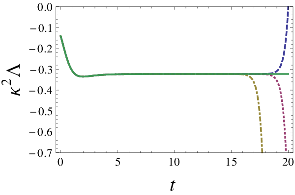
It is very tempting to assume $c\neq 0$ , and get the asymptotic solution for $\kappa\rightarrow\infty$

\displaystyle\kappa^{2}\Lambda(\kappa)

\displaystyle\sim

\displaystyle-\frac{1}{4}\left(29+5\sqrt{\frac{215}{7}}\right).

(85)

Numerical investigations, Fig. 8, of the solution to the “full” equation, where we have not made the asymptotic expansion, starting the integration from $t=\ln(\kappa)=20$ , shows that when we have chosen an arbitrary initial condition at finite $\kappa$ , the solution typically has a quick decay to the fixed point value for $c=0$ , for almost all initial conditions. Only when we start very close to the asymptotic value (85) do we find an apparently divergent numerical solution. Thus it is actually most efficient to use the asymptotic solution with the choice $c=0$ ,

\kappa^{2}\Lambda(\kappa)\sim-\frac{1}{4}\left(29-5\sqrt{\frac{215}{7}}\right),

(86)

as initial condition for large $\kappa$ .

The differential equation for $\Lambda^{\prime}$ does not have such a trivial fixed point; the asymptotic solution is found to be quasi-periodic

\kappa^{2}\Lambda^{\prime}(\kappa)=\frac{1}{28}\left(31+5\sqrt{535}\tan\left(\frac{1}{25}\sqrt{535}\ln(\kappa)+\phi_{0}\right)\right).

(87)

This limit cycle-behaviour is the basic manifestation of the Efimov effect in the approach employed here.

A.1.2 Four-body couplings

For the fur body-couplings we can also define scaled integrals,

$\displaystyle\tilde{K}_{1}$	$\displaystyle=$	$\displaystyle\frac{192\pi^{2}\kappa^{4}\left(\kappa^{2}+1\right)^{3}}{5\left(3\left(\kappa^{2}+1\right)^{2}\cot^{-1}(\kappa)+\kappa\left(5\kappa^{2}+3\right)\right)}$	(88)
		$\displaystyle\times\frac{\left(15\left(\kappa^{2}+1\right)^{3}\cot^{-1}(\kappa)+\kappa\left(17\kappa^{4}+40\kappa^{2}+15\right)\right)}{\left(3\left(\kappa^{2}+1\right)^{2}\left(\kappa^{2}+8\right)\cot^{-1}(\kappa)+\kappa\left(21\kappa^{4}+43\kappa^{2}+24\right)\right)^{2}},$	(88)
$\displaystyle\tilde{K}_{2}$	$\displaystyle=$	$\displaystyle\frac{4\kappa^{4}}{3\pi^{2}\left(\kappa^{2}+1\right)^{3}},$	(89)
$\displaystyle\tilde{K}_{3}$	$\displaystyle=$	$\displaystyle\frac{8\kappa^{4}}{3\pi^{2}\left(\kappa^{2}+1\right)^{4}}.$	(90)

We can rewrite the differential equations as

	$\displaystyle\partial_{\kappa}\bar{U}_{2}$	$\displaystyle=\frac{1}{2}\bar{U}_{2}^{2}\tilde{K}_{1}-2\Lambda^{\prime}\tilde{K}_{2}+\frac{3}{2}\tilde{K}_{3},$		(91)
	$\displaystyle\partial_{\kappa}U_{2}$	$\displaystyle=\frac{1}{2}U_{2}^{2}\tilde{K}_{1}-2\Lambda\tilde{K}_{2}-\frac{3}{4}\tilde{K}_{3},$		(92)

and the asymptotic expansions

$\displaystyle\tilde{K}_{1}$	$\displaystyle=$	$\displaystyle\frac{4\pi^{2}\kappa^{2}}{15},$	(93)
$\displaystyle\tilde{K}_{2}$	$\displaystyle=$	$\displaystyle\frac{4}{3\pi^{2}\kappa^{2}},$	(94)
$\displaystyle\tilde{K}_{3}$	$\displaystyle=$	$\displaystyle\frac{8}{3\pi^{2}\kappa^{4}}.$	(95)

It pays off to use

V_{DD}(\kappa)=\kappa^{3}\bar{U}_{2}

(96)

This satisfies

\kappa\partial_{\kappa}V_{DD}=\frac{2\pi^{4}}{15}V_{DD}(\kappa)^{2}+3V_{DD}(\kappa)+\frac{4}{\pi^{2}}-\frac{8}{5\pi^{2}}\kappa^{2}\Lambda^{\prime}(\kappa).

(97)

Without the additional $\Lambda$ term we find for large $\kappa$ that

V_{DD}\rightarrow-\frac{45+\sqrt{1545}}{4\pi^{2}}\approx-2.13551.

(98)

By numerical solution we find that the periodic oscillations in $\Lambda$ dominate over this behaviour.

A.2 Scattering lengths

A.2.1 Dimer-dimer scattering

Our effective action contains the term

$\displaystyle V_{DD}=$	$\displaystyle\frac{1}{2}u_{2}\int\delta^{(4)}(p_{1}+p_{3}-p_{2}-p_{4})\left[\phi_{\alpha}^{\dagger}(p_{10},\boldsymbol{p}_{1})\phi_{\alpha}(p_{20},\boldsymbol{p}_{2})\right]\left[\phi_{\beta}^{\dagger}(p_{30},\boldsymbol{p}_{3})\phi_{\beta}(p_{40},\boldsymbol{p}_{4})\right]$
	$\displaystyle+\frac{1}{12}u_{2}^{{}^{\prime}}\int\delta^{(4)}(p_{1}+p_{2}-p_{3}-p_{4})\left[\boldsymbol{t}^{\dagger}(p_{10},\boldsymbol{p}_{1})\cdot\boldsymbol{t}^{\dagger}(p_{20},\boldsymbol{p}_{2})-\boldsymbol{s}^{\dagger}(p_{10},\boldsymbol{p}_{1})\cdot\boldsymbol{s}^{\dagger}(p_{20},\boldsymbol{p}_{2})\right]$
	$\displaystyle\qquad\times\left[\boldsymbol{t}(p_{30},\boldsymbol{p}_{3})\cdot\boldsymbol{t}(p_{40},\boldsymbol{p}_{4})-\boldsymbol{s}(p_{30},\boldsymbol{p}_{3})\cdot\boldsymbol{s}(p_{40},\boldsymbol{p}_{4})\right].$	(99)

This is in terms of classical fields; the corresponding operator in the “pole approximation” when the cut-off reaches zero is

$\displaystyle\hat{V}_{DD}=$	$\displaystyle\frac{1}{2}u_{2}^{\prime}:\hat{n}^{2}:$
	$\displaystyle+\frac{1}{12}u_{2}\left[\hat{\boldsymbol{t}}^{\dagger}(E_{B},0)\cdot\hat{\boldsymbol{t}}^{\dagger}(E_{B},0)-\hat{\boldsymbol{s}}^{\dagger}(E_{B},0)\cdot\hat{\boldsymbol{s}}^{\dagger}(E_{B},0)\right]$	(100)
	$\displaystyle\quad\left[\hat{\boldsymbol{t}}(E_{B},0)\cdot\hat{\boldsymbol{t}}(E_{B},0)-\hat{\boldsymbol{s}}(E_{B},0)\cdot\hat{\boldsymbol{s}}(E_{B},0)\right]$
$\displaystyle=$	$\displaystyle\frac{1}{2}u_{2}^{\prime}\hat{n}\left(\hat{n}-1\right)$
	$\displaystyle+\frac{1}{12}u_{2}\left[\hat{\boldsymbol{t}}^{\dagger}(E_{B},0)\cdot\hat{\boldsymbol{t}}^{\dagger}(E_{B},0)-\hat{\boldsymbol{s}}^{\dagger}(E_{B},0)\cdot\hat{\boldsymbol{s}}^{\dagger}(E_{B},0)\right]$	(101)
	$\displaystyle\quad\left[\hat{\boldsymbol{t}}(E_{B},0)\cdot\hat{\boldsymbol{t}}(E_{B},0)-\hat{\boldsymbol{s}}(E_{B},0)\cdot\hat{\boldsymbol{s}}(E_{B},0)\right].$	(102)

Note the important effect of normal ordering; this is simply a re-statement of the fact that $u_{2}^{\prime}$ does not contribute in the single dimer channels. We now calculate the scattering between the normalised scalar ( $[2]$ denotes the symmetric irrep of SU(4) [39]) states

\left|[2](0,0)\right\rangle=\frac{1}{\sqrt{6\times 2}}\left[\hat{\boldsymbol{t}}^{\dagger}(E_{B},0)\cdot\hat{\boldsymbol{t}}^{\dagger}(E_{B},0)-\hat{\boldsymbol{s}}^{\dagger}(E_{B},0)\cdot\hat{\boldsymbol{s}}^{\dagger}(E_{B},0)\right]\left|0\right\rangle,

(103)

and we get

\left\langle[2](0,0)\right|V_{DD}\left|[2](0,0)\right\rangle=\bar{u}_{2}.

(104)

We thus find that

	$\displaystyle a_{DD}$	$\displaystyle=\frac{M_{B}}{4\pi}\bar{u}_{2}/Z_{\phi}^{2}=\frac{M_{{N}}}{2\pi}\bar{u}_{2}/Z_{\phi}^{2}$
		$\displaystyle=a_{t}32\pi(\bar{U}_{2})$		(105)

We also use the fact that $Z_{\phi}(0)=a_{t}g^{2}M^{2}/8\pi$ .

In the same vein we find in the other channel ( $[1,1]$ denotes the antisymmetric irrep of SU(4))

\left|[1,1](0,0)\right\rangle=\frac{1}{\sqrt{6\times 2}}\left[\hat{\boldsymbol{t}}^{\dagger}(E_{B},0)\cdot\hat{\boldsymbol{t}}^{\dagger}(E_{B},0)+\hat{\boldsymbol{s}}^{\dagger}(E_{B},0)\cdot\hat{\boldsymbol{s}}^{\dagger}(E_{B},0)\right]\left|0\right\rangle,

(106)

that

	$\displaystyle a_{DD}^{AS}$	$\displaystyle=\frac{M_{B}}{4\pi}u_{2}/Z_{\phi}^{2}=\frac{M_{{N}}}{2\pi}u_{2}/Z_{\phi}^{2}$
		$\displaystyle=a_{t}32\pi(U_{2})$		(107)

In the mean-field limit, we find that $\lim_{\kappa\rightarrow 0}U_{2}=1/16\pi$ , and we get the standard result $a_{DD}^{AS}=2a_{t}$ .

A.2.2 Dimer-nucleon scattering

There are two possible dimer-nucleon state we can construct, a symmetric and antisymmetric one.

We first assume that the scattering is evaluated in the channel of the symmetric dimer-nucleon states

\left|DN\right\rangle=\frac{1}{\sqrt{2}}\left[\hat{t}^{\dagger}(E_{B},0)\hat{\psi}^{\dagger}(E_{B}/2,0)-\hat{s}^{\dagger}(E_{B},0)\hat{\psi}^{\dagger}(E_{B}/2,0)\right]_{m_{S},m_{s}}^{1/2,1/2}\left|0\right\rangle,

(108)

we get

\left\langle DF\right|\hat{t}\left|DF\right\rangle=\lambda.

(109)

We thus conclude

	$\displaystyle a_{DN}$	$\displaystyle=\frac{M_{red}}{4\pi}\lambda/Z_{\phi}=\frac{2M_{{N}}/3}{4\pi}\lambda/Z_{\phi}$
		$\displaystyle=a_{t}\frac{4}{3}\Lambda.$		(110)

In the antisymmetric case, defined by

\left|DN^{\prime}\right\rangle=\frac{1}{\sqrt{2}}\left[\hat{t}^{\dagger}(E_{B},0)\hat{\psi}^{\dagger}(E_{B}/2,0)+\hat{s}^{\dagger}(E_{B},0)\hat{\psi}^{\dagger}(E_{B}/2,0)\right]_{m_{S},m_{s}}^{1/2,1/2}\left|0\right\rangle,

(111)

we get

	$\displaystyle a_{DN}^{\prime}$	$\displaystyle=\frac{M_{red}}{4\pi}\lambda^{\prime}/Z_{\phi}=\frac{2M_{{N}}/3}{4\pi}\lambda^{\prime}/Z_{\phi}$
		$\displaystyle=a_{t}\frac{4}{3}\Lambda^{\prime}.$		(112)

Appendix B Link between $T$ and $V$

Our main results are for the threshold behaviour of various quantities are, in the main, expressed in terms of scattering lengths. The relation between our effective action and a scattering length is based on the definition

\lim_{k\rightarrow 0}T(k)=\frac{2\pi}{M_{red}}a_{t}.

(113)

For identical mass, $M_{1}=M_{2}=M$ , we get

T(0)=\frac{4\pi}{M}a_{t}.

(114)

What we call a “potential” in the effective action, is really nothing but the classical form of the $T$ matrix. For dimers we find a similar relation, but we have to interpret $T$ as the expectation value of the quantised potential in the relevant channel. As shown in the appendix, this allows us to take into account symmetry aspects of the problem. Thus

V=\left\langle\hat{V}\right\rangle=T_{DD}(0)=\frac{4\pi a_{{D}D}}{M_{{D}}},

(115)

which can be used to show that the dimer-dimer scattering length in the mean-field limit goes to $2a_{t}$ .

References

[1] C. Wetterich, Phys. Lett. B301, 90 (1993).
[2] T. Morris, Phys. Lett. B334, 355 (1994).
[3] J. Berges, N. Tetradis and C.Wetterich, Phys. Rept. 363, 223 (2002).
[4] B. Delamotte, D. Mouhanna and M. Tissier, Phys. Rev. B 69, 134413 (2004).
[5] J. M. Pawlowski, Ann. Phys.322, 2831 (2007).
[6] S. Diehl, H. C. Krahl, and M. Scherer, Phys. Rev. C78, 034001 (2008).
[7] S. Moroz, S. Floerchinger, R. Schmidt, C. Wetterich, Phys. Rev. A79, 042705 (2009).
[8] R. Schmidt and S. Moroz, Phys. Rev. A 81, 052709 (2010).
[9] B. Krippa, N. R. Walet, M. C. Birse, Phys. Rev. A81 043628 (2010).
[10] M. C. Birse, B. Krippa and N. R. Walet, Phys. Rev. A83 023621 (2011).
[11] G. V. Skorniakov and K. A. Ter-Martirosian, Sov. Phys. JETP 4, 648 (1957).
[12] V. N. Efimov, Yad. Fiz. 12, 1080 (1970) [Sov. J. Nucl. Phys. 12, 589 (1971)].
[13] M. C. Birse, B. Krippa, J. A. McGovern and N. R. Walet, Phys. Lett. B605, 287 (2005).
[14] H.Gies, “Introduction to the functional RG and applications to gauge theories”, Lectures held at the 2006 ECT School “Renormalization Group and Effective Field Theory Approaches to Many-Body Systems”, Trento, Italy [arXiv:hep-ph/0611146].
[15] S. Diehl, H. Gies, J. M. Pawlowski, and C. Wetterich, Phys. Rev. A 76, 021602 (2007).
[16] E. Wigner, Phys. Rev. 51, 106 (1937).
[17] T. Mehen, I. W. Stewart, and M. B. Wise, Phys. Rev. Lett. 83, 931 (1999).
[18] S. Weinberg, The quantum theory of fields, Vol. 2, Chapter 16 (Cambridge University Press, 1996).
[19] K. G. Wilson and J. G. Kogut, Phys. Rep. 12C, 75 (1975).
[20] J. Berges, N. Tetradis and C. Wetterich, Phys. Rept. 363, 223 (2002).
[21] B. Delamotte, D. Mouhanna and M. Tissier, Phys. Rev. B69, 134413 (2004).
[22] S. R. Beane et al., in At the Frontier of Particle Physics: Handbook of QCD, edited by M. Shifman (World Scientific, Singapore, 2001), Vol. 1, p. 133.
[23] P. F. Bedaque and U. van Kolck, Ann. Rev. Nucl. Part. Sci. 52, 339 (2002).
[24] P. F. Bedaque, H.-W. Hammer, and U. van Kolck, Nucl. Phys. A 676, 357 (2000).
[25] D. B. Kaplan, Nucl. Phys. B494, 471 (1997).
[26] D. F. Litim, Phys. Rev. D 64, 105007 (2001).
[27] M. C. Birse, Phys. Rev. C 77, 047001 (2008).
[28] A.C. Phillips, Nucl. Phys. A 107, 209 (1968) [CAS].
[29] J. A. Tjon. Phys. Lett. B 56, 217, (1975).
[30] W. Dilg, L. Koester, and W. Nistler, Phys. Lett. B36, 208 (1971).
[31] J.L. Friar, B.F. Gibson, G.L. Payne, C.R. Chen, Phys. Lett. B 247, 197 (1990).
[32] F. Ciesielski, J. Carbonell, and C. Gignoux. Phys. Lett. B 447, 199 (1999).
[33] S. Diehl, H. C. Krahl and M. Scherer,Phys.Rev.C78, 034001 (2008).
[34] L. Berezhiani, G. Gabadadze and D. Pirtskhalava, JHEP 04, 122 (2010).
[35] I.N. Filikhin and S. L. Yakovlev, Yad. Fiz. 63, 271 (2000) [Phys. At. Nucl. 63, 216 (2000)].
[36] F. Ciesielski and J. Carbonell, Phys. Rev. C 58, 58 (1998)
[37] G. Rupak, arXiv:nucl-th/0605074
[38] P. F. Bedaque, U. van Kolck, Phys. Lett. B 428, 221 (1998); P.F. Bedaque, H.-W. Hammer, U. van Kolck, Phys. Rev. C 58, 641 (1998).
[39] Brian G. Wybourne, Classical groups for physicists (Wiley, 1974)

Functional renormalisation group for few-nucleon systems: SU(4) symmetry and its breaking