A Framework of Algorithms: Computing the Bias and Prestige of Nodes in Trust Networks

Rong-Hua Li Jeffrey Xu Yu Xin Huang Hong Cheng Address: The Chinese University of Hong Kong Email: {rhli,yu,xhuang,hcheng}@se.cuhk.edu.hk

Abstract

A trust network is a social network in which edges represent the trust relationship between two nodes in the network. In a trust network, a fundamental question is how to assess and compute the bias and prestige of the nodes, where the bias of a node measures the trustworthiness of a node and the prestige of a node measures the importance of the node. The larger bias of a node implies the lower trustworthiness of the node, and the larger prestige of a node implies the higher importance of the node. In this paper, we define a vector-valued contractive function to characterize the bias vector which results in a rich family of bias measurements, and we propose a framework of algorithms for computing the bias and prestige of nodes in trust networks. Based on our framework, we develop four algorithms that can calculate the bias and prestige of nodes effectively and robustly. The time and space complexities of all our algorithms are linear w.r.t. the size of the graph, thus our algorithms are scalable to handle large datasets. We evaluate our algorithms using five real datasets. The experimental results demonstrate the effectiveness, robustness, and scalability of our algorithms.

1 Introduction

Online social networks (OSNs) such as Facebook, Twitter, and MySpace have become increasingly popular in recent years. These OSNs provide users with various utilities to share all sorts of information with friends, such as thoughts, activities, photos, etc. As a new way to express information, trust networks such as Advogato (www.advogato.org), Kaitiaki (www.kaitiaki.org.nz), Epinions (www.epinions.com), and Slashdot (www.slashdot.org) rapidly attract more and more attention. Unlike the traditional OSNs where edges represent the friendship between users, in the trust networks, edges express the trust relationship between two users. In other words, users express their trust to other users by giving a trust score to another, and users are evaluated by others based on their trust scores. There exist two types of trust networks, namely, unsigned and signed. In the unsigned trust networks, such as Advogato and Kaitiaki, users can only express their trust to other users by giving a non-negative trust score to others. In the signed trust networks, such as Epinions and Slashdot, users can express their trust or distrust to others by giving a positive or negative trust score to others. There are many applications in the trust networks, such as finding the trusted nodes in a network [23], predicting the trust score of the nodes, and the trust based recommendation systems [21].

In a signed/unsigned trust network, the final trustworthiness of a user is determined by how users trust each other in a global context, and is measured by bias. The bias of a user reflects the extent up to which his/her opinions differ from others. If a user has a zero bias, then his/her opinions are 100% unbiased and can be 100% taken. Consequently, the user has high trustworthiness. On the other hand, if a user has a large bias, then his/her opinions cannot be 100% taken because his/her opinions are often different from others. Therefore, the user has low trustworthiness. Another important measure, the prestige of a user, reflects how he/she is trusted by others (the importance). In this work, we study how to assess and compute the bias and prestige of the users. The challenges are: (1) how to define a reasonable bias measurement that can capture the bias of the users’ opinions, (2) how to handle the negative trust scores in signed trust networks, and (3) how to design a robust algorithm that can prevent attack from some adversarial users.

As pointed out in [23], the traditional eigenvector based methods, such as eigenvector centrality [4], HITS [5], and PageRank [17], cannot be directly used to solve this problem. The reason is of twofold. First, the eigenvector based methods typically cannot handle the negative edges. Moreover, they cannot distinguish the two cases, namely non-connection and zero trust score, where a zero trust score implies that there is an edge from a user to another user with the zero trust score (e.g., $W_{32}$ in Fig. 1). Second, they ignore the bias of the nodes. To the best of our knowledge, the algorithm proposed by Mishra and Bhattacharya [23] is the only algorithm that addresses this problem. We refer to this algorithm as the MB algorithm (or simply MB). MB is tailored for the signed trust networks, and can also be used for the unsigned trust networks. However, MB has major drawbacks. The trustworthiness of a user cannot be trusted due to the fact that MB treats bias of a user by relative differences between itself and others. For instance, if a user gives all his/her friends a much higher trust score than the average of others, and gives all his/her foes a much lower trust score than the average of others, such differences cancel out, which leads to a zero bias for the user. This cancellation happens in either a signed or a unsigned trust network. Therefore, MB can be attacked by the adversarial users. We will analyze it in Section 3 in detail.

In this paper, we propose new bias measurements to capture the bias of the users’ opinions. First, we define a vector-valued contractive function as a framework to represent the bias vector, which implies a rich family of bias measurements and thereby results in a rich family of algorithms. On the basis of our framework, we develop four new bias measurements using absoluate differences instead of relative differences to deal with bias, in order to avoid such a cancellation problem in MB. Based on the bias of the nodes, the trustworthiness score of a node is inversely proportional to the bias score of the node, and the prestige of a node is the average trustworthiness-weighted trust scores. In other words, if a node is with a large bias score, then the trust scores given by this node will be assigned to small weights. Our algorithms iteratively refine the bias and prestige scores of the nodes. The final bias and prestige vector is obtained when the algorithm converges. The main contributions of this paper are summarized as follows.

•

First, we propose a framework of algorithms for computing the bias and prestige of the nodes in either unsigned or signed trust networks. We rigorously prove the convergence properties of our framework.
•

Second, based on the proposed framework, we show that MB [23] is a special case of our framework for unsigned trust networks. We also develop four new algorithms that can overcome the cancellation problem in MB. The bias measurements of our new algorithms are more reasonable, and our algorithms are more effective and more robust than MB.
•

Third, we conducted extensive experimental studies to confirm the effectiveness, robustness, and scalability of the proposed algorithms. We compare our algorithms with the state-of-the-art algorithm (MB) over five real datasets. The results indicate that our newly proposed algorithms outperform MB in terms of both effectiveness and robustness. We also evaluate the scalability of the proposed algorithms, and the results demonstrate the scalability of our algorithms is linear w.r.t. the size of the graphs.

The rest of this paper is organized as follows. We introduce the related work in Section 2. We give the preliminaries and problem statement, and discuss the drawbacks of the existing algorithms in Section 3. We propose and analyze the algorithm framework as well as four novel specific algorithms in Section 4. Extensive experimental results are presented in Section 5. Finally, we conclude this work in Section 6.

2 Related work

Our work is closely related to graph-based ranking algorithms. In the last decades, ranking nodes in networks has attracted much attention in both research and industry communities. There are a large number of algorithms, such as HITS [17], PageRank [5] and its variants [10, 12]. Most of these ranking algorithms are based on the spectral of the adjacency matrix of the network. A survey on using spectral techniques for ranking can be found in [27]. However, all of these algorithms only focus on finding the prestige of the nodes in the networks, and do not consider the bias of the nodes, thus cannot be directly used in our problem. In addition, the convergence of these algorithms is guaranteed by the non-negative matrix theory [18]. Therefore, they cannot be directly generalized to the signed trust networks [20], where the edges are possibly associated with a negative weight. A straightforward method is to remove the negative edges, and then perform the ranking algorithms on the non-negative graph. Obviously, this method ignores the negative relationship between the nodes of the graph, and may result in poor ranking performance [9]. To address this issue, de Kerchove et al. [6] propose a Pagetrust algorithm, which can handle the negative edges, but the convergence of their algorithm cannot be guaranteed.

Our work is also related to the trust management [14, 29, 13, 3]. Richardson et al. in [25] propose an eigenvector based algorithm for the trust management in semantic web. Independent to Richardson’s work, Kamvar et al. in [15] present a similar eigenvector based algorithm, namely Eigentrust, for the trust management in P2P networks. Guha et al. in [9] study the problem of propagation of trust and distrust in the networks. Subsequently, Theodorakopoulos et al. in [26] study the trust model and trust evaluation metrics from an algebra viewpoint. They use semiring to express a trust model and then model the trust evaluation problem as a path problem on a directed graph. Recently, Andersen et al. in [1] propose an axiomatic approach for the trust based recommendation systems [21]. All of these algorithms are based on the spectral techniques, and cannot be easily generalized to the signed networks. There also exist trust based ranking algorithms [22]. These algorithms are designed based on the same idea “the users whose opinions often differ from the others’ opinions will be assigned to less trust scores”. In the literature, such algorithms include [24, 19, 28, 7, 30]. All of these algorithms are tailored for the bipartite rating networks, and generalization to the general networks would be meaningless. Moreover, all of them except [7] cannot guarantee the convergence. As an exception, in [7], de Kerchove and Dooren prove the convergence of their algorithm, but the rate of the convergence is q-linear. In addition, the convergence property of their algorithm [7] is dependent on the decay constant, which is very hard to be determined in practice.

3 Preliminaries

We model a trust network as a directed weighted graph $G=(V,E,W)$ with $n$ nodes and $m$ edges, where $V$ represents the node set, $E$ denotes the edge set, and $W$ denotes the weights. In graph $G$ , a weight $W_{ij}$ signifies a trust score from node $i$ to node $j$ . All trust scores are normalized in the range of $[0,1]$ . For simplicity, in the following discussions, we focus on an unsigned trust network assuming that all edge-weights are non-negative. Our approaches can be readily generalized to signed trust networks, and we will discuss it in Section 4.4.

An example is shown in Fig. 1. In Fig. 1, node 5 gives a trust score 0.1 to node 1 ( $W_{51}=0.1$ ), whereas two nodes, 2 and 3, give a high trust score 0.8 to node 1 ( $W_{21}=W_{31}=0.8$ ). And node 5 gives a trust score 0.9 to node 3 ( $W_{53}=0.9$ ), while two nodes, 2 and 4, give a low trust score to node 3 instead ( $W_{23}=W_{43}=0.2$ ). This observation shows that node 5’s opinions often differ from those of others, thus indicates that node 5 is a biased node. On the other hand, there are two nodes (2 and 3) giving a high trust score 0.8 to node 1 ( $W_{21}=W_{31}=0.8$ ), which suggests that node 1 would be a prestigious node. Additionally, in this example, node 3 gives 0 to node 2 ( $W_{32}=0$ ), which implies that node 3 does not trust node 2 at all.

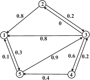
Refer to caption — Figure 1: A trust network.

Given a trust network $G$ , the problem we study is how to compute the bias and prestige of the nodes based on the trust scores. As discussed, the eigenvector based methods are not applicable, and the only existing solution is MB [23]. In the following, we briefly review MB and discuss its major drawbacks.

In MB, each node has two scores: the bias and prestige score. The bias and prestige scores of node $i$ are denoted by $b_{i}$ and $r_{i}$ , respectively. Formally, the bias of node $i$ is defined by

b_{i}=\frac{1}{{2|O_{i}|}}\sum\limits_{j\in O_{i}}{(W_{ij}-r_{j})},

(1)

where $O_{i}$ denotes the set of all outgoing neighbors of node $i$ . The idea behind is that a node will be assigned to a high bias score if it often behaves differently from others. The prestige score of node $i$ ( $r_{i}$ ) is given by

r_{i}=\frac{1}{{|I_{i}|}}\sum\limits_{j\in I_{i}}{(W_{ji}(1-\max\{0,b_{j}\times sign(W_{ji})\}))},

(2)

where $I_{i}$ denotes the set of all incoming neighbors of node $i$ , and $sign(W_{ji})$ denotes the sign of an edge from node $j$ to node $i$ , which can be positive (trust) or negative (distrust).

The MB algorithm works in an iterative fashion, and the corresponding iterative system is

\left\{\begin{array}[]{l}r_{i}^{k+1}=\frac{1}{{|I_{i}|}}\sum\limits_{j\in I_{i}}{(W_{ji}(1-\max\{0,b_{j}^{k}\times sign(W_{ji})\}))}\\ b_{j}^{k+1}=\frac{1}{{2|O_{j}|}}\sum\limits_{i\in O_{j}}{(W_{ji}-r_{i}^{k+1})}\\ \end{array}\right.

(3)

There are two major drawbacks in MB. First, in Eq. (1), the differences ( $W_{ij}-r_{j}$ ) for different outgoing neighbors $j\in O_{i}$ can be canceled out, thus will result in unreasonable bias measures. Reconsider the example (Fig. 1), node 5 gives 0.1 to node 1, while both node 2 and node 3 give 0.8 to node 1. With these three edges ( $5\rightarrow 1$ , $2\rightarrow 1$ , and $3\rightarrow 1$ ), the trust score given by node 5 is significantly lower than those of others with a difference $0.1-0.8=-0.7$ . However, consider the other three edges $2\rightarrow 3$ , $4\rightarrow 3$ , and $5\rightarrow 3$ , we can find that the trust score given by node 5 is significantly larger than those of the other two nodes (nodes 2 and 4) with a difference 0.7. The positive and negative differences can be canceled out by Eq. (1), and this will cause node 5 to be trusted with a lower bias score. However, intuitively, node 5’s opinions often differ from those of others, thereby it should be assigned to a large bias score. Table 1 shows the bias scores by MB after each iteration. We can clearly see that node 5 gets the minimal bias scores (0.014), which contradicts to the intuition.

Table 1: Bias scores by the MB algorithm.

Iteration	node 1	node 2	node 3	node 4	node 5
1	0.350	0.042	0.121	0.250	0.042
2	0.350	0.015	0.129	0.232	0.015
3	0.350	0.014	0.129	0.231	0.014
4	0.350	0.014	0.129	0.231	0.014

Second, as also pointed in [23], MB is easy to be attacked by the adversarial nodes. For example, some nodes can maintain their bias scores closely to 0 by giving high trust scores to the nodes with low prestige scores and giving the low trust scores to the nodes with high prestige scores (as node 5 in Fig. 1). In [23], Mishra and Bhattacharya present a statistical method for detecting such adversarial nodes. But the statistical method is independent to MB, thus it cannot reduce the influence of the adversarial nodes in MB. In addition, the proof for the convergence of the MB presented in [23] is not rigorous. In the present paper, we rigorously prove the convergence of our framework using the Cauthy convergence theorem [2].

4 Our New Approach

In this section, we propose a framework of algorithms for computing the bias and prestige of the nodes in trust networks. In our framework, every node $i$ has two scores: the bias score ( $b_{i}$ ) and the prestige score ( $r_{i}$ ). We use two vectors $b$ and $r$ to denote the bias vector and prestige vector, respectively. Specifically, we define the bias of node $j$ by

b_{j}=(f(r))_{j},

(4)

where $r$ is the prestige vector of the nodes, $f(r):\mathbb{R}^{n}\to\mathbb{R}^{n}$ is a vector-valued contractive function, which is defined in Definition 4.1, and $(f(r))_{j}$ denotes the $j$ -th element of vector $f(r)$ . We restrict $0\leq f(r)\leq e$ , where $e\in\mathbb{R}^{n}$ and $e=[1,1,\cdots,1]^{T}$ .

Definition 4.1.

For any $x,y\in\mathbb{R}^{n}$ , the function $f:\mathbb{R}^{n}\to\mathbb{R}^{n}$ is a vector-valued contractive function if the following condition holds.

|f(x)-f(y)|\leq\lambda||x-y||_{\infty}e

(5)

where $\lambda\in[0,1)$ , $||\bullet||_{\infty}$ denotes the infinity norm.

Since $\lambda\in[0,1)$ , the vector-valued function $f$ exhibits contractive property w.r.t. the infinity norm of the vector, we refer to it as the vector-valued contractive function. It is worth noting that the vector-valued contractive function we define is a generalization of the contraction mapping in the fixed point theory [8]. In [8], the contraction mapping is defined on a 1-dimensional variable and the domain of the contraction mapping is also a 1-dimensional value. Our vector-valued contractive function is defined on an $n$ -dimensional vector and its domain is also an $n$ -dimensional vector. The contraction mapping is very useful for iterative function systems [8]. Our vector-valued contractive function sheds light on studying the iterative vector-valued function systems in trust networks.

As can be seen in Eq. (4), the bias vector $b$ is obtained by a vector-valued contractive function defined on the prestige vector $r$ . The advantage of the definition of bias is that it makes our framework general, which will result in a rich family of bias measurements. In Section 4.2, we will give four different bias measurements and each of these measurements is shown to be a vector-valued contractive function.

With the bias of the nodes, the trustworthiness of node $j$ is given by $1-b_{j}$ , which is inversely proportional to the bias score of node $j$ . We compute the prestige score of node $i$ by averaging the trustworthiness-weighted trust scores given by the incoming neighbors of node $i$ . In particular, the prestige score $r_{i}$ for a node $i$ is given by

r_{i}=\frac{1}{{|I_{i}|}}\sum\limits_{j\in I_{i}}{W_{ji}(1-(f(r))_{j})},

(6)

where $I_{i}$ is the set of all incoming neighbors of node $i$ . Our algorithm iteratively refines the prestige vector and the bias vector using the following iterative system:

\left\{\begin{array}[]{l}r_{i}^{k+1}=\frac{1}{{|I_{i}|}}\sum\limits_{j\in I_{i}}{W_{ji}(1-b_{j}^{k})}\\ b_{j}^{k+1}=(f(r^{k+1}))_{j}\\ \end{array}\right.

(7)

where $r_{i}^{k+1}$ denotes the prestige of node $i$ in the $(k$ + $1)$ -th iteration and $b_{j}^{k+1}$ denotes the bias of node $j$ in the $(k$ + $1)$ -th iteration. Initially, we set $f(r^{0})=0$ , which implies $0\leq r^{k}\leq 1$ . The iterative system (Eq. (7)) will converge into a unique fixed prestige and bias vector in an exponential rate of convergence, as we will show in Section 4.1.

4.1 Analysis of the proposed algorithm

Convergence of the proposed algorithm: We analyze the convergence properties of the iterative system described in Eq. (7). Specifically, we show the prestige vector will converge into a unique fixed point as stated in Theorem 4.3. Similar arguments can be used to prove the bias vector also converges into a unique fixed point. First, we prove the following lemma.

Lemma 4.2.

For any node $i$ , $|r_{i}^{k+1}-r_{i}^{k}|\leq\lambda^{k}||r^{1}-r^{0}||_{\infty}$ .

Proof: We prove Lemma 4.2 by induction. Let $k=1$ , we have

\begin{array}[]{l}|r_{i}^{2}-r_{i}^{1}|=|\frac{1}{{|I_{i}|}}\sum\limits_{j\in I_{i}}{W_{ji}((f(r^{0}))_{j}-(f(r^{1}))_{j})}|\\ \quad\quad\quad\;\;\;\leq\frac{1}{{|I_{i}|}}\sum\limits_{j\in I_{i}}{W_{ji}|(f(r^{0}))_{j}-(f(r^{1}))_{j}|}\\ \quad\quad\quad\;\;\;\leq\frac{\lambda}{{|I_{i}|}}\sum\limits_{j\in I_{i}}{W_{ji}||r^{1}-r^{0}||_{\infty}}\\ \quad\quad\quad\;\;\;\leq\lambda||r^{1}-r^{0}||_{\infty},\\ \end{array}

where the second inequality is due to the definition of vector-valued contractive function, and the last inequality is by $|W_{ij}|\in[0,1]$ . Assume the lemma holds when $k=t$ . We show that the lemma still holds when $k=t+1$ .

\begin{array}[]{l}|r_{i}^{t+2}-r_{i}^{t+1}|=|\frac{1}{{|I_{i}|}}\sum\limits_{j\in I_{i}}{W_{ji}((f(r^{t}))_{j}-(f(r^{t+1}))_{j})}|\\ \quad\quad\quad\quad\quad\;\;\;\leq\frac{1}{{|I_{i}|}}\sum\limits_{j\in I_{i}}{W_{ji}|(f(r^{t}))_{j}-(f(r^{t+1}))_{j}|}\\ \quad\quad\quad\quad\quad\;\;\;\leq\frac{\lambda}{{|I_{i}|}}\sum\limits_{j\in I_{i}}{W_{ji}||r^{t+1}-r^{t}||_{\infty}}\\ \quad\quad\quad\quad\quad\;\;\;\leq\lambda||r^{t+1}-r^{t}||_{\infty}\\ \quad\quad\quad\quad\quad\;\;\;\leq\lambda^{t+1}||r^{1}-r^{0}||_{\infty},\\ \end{array}

where the second inequality is due to the definition of vector-valued contractive function and the last inequality holds by the induction assumption. This completes the proof. $\Box$

With Lemma 4.2, we prove the convergence property.

Theorem 4.3.

The iterative system defined in Eq. (7) converges into a unique fixed point.

Proof: We first prove the convergence of the iterative system (Eq. (7)), and then prove the uniqueness. Specifically, for $\varepsilon>0$ , there exists $N$ such that

\lambda^{N}<\frac{{(1-\lambda)\varepsilon}}{{||r^{1}-r^{0}||_{\infty}}}.

Then, for any $s>t\geq N$ , we have

\begin{array}[]{l}|r_{i}^{s}-r_{i}^{t}|\leq|r_{i}^{s}-r_{i}^{s-1}|+|r_{i}^{s-1}-r_{i}^{s-2}|+\cdots+|r_{i}^{t+1}-r_{i}^{t}|\\ \quad\quad\quad\;\;\;\leq\lambda^{s-1}||r^{1}-r^{0}||_{\infty}+\lambda^{s-2}||r^{1}-r^{0}||_{\infty}+\cdots+\\ \quad\quad\quad\quad\quad\lambda^{t}||r^{1}-r^{0}||_{\infty}\\ \quad\quad\quad\;\;\;\leq||r^{1}-r^{0}||_{\infty}\lambda^{t}\sum\limits_{k=0}^{s-t-1}{\lambda^{k}}<||r^{1}-r^{0}||_{\infty}\lambda^{t}\sum\limits_{k=0}^{\infty}{\lambda^{k}}\\ \quad\quad\quad\;\;\;=||r^{1}-r^{0}||_{\infty}\lambda^{t}\frac{1}{{1-\lambda}}\\ \quad\quad\quad\;\;\;\leq||r^{1}-r^{0}||_{\infty}\lambda^{N}\frac{1}{{1-\lambda}}\\ \quad\quad\quad\;\;\;\leq\varepsilon,\\ \end{array}

where the first inequality holds by the triangle inequality, and the second inequality is due to Lemma 4.2. Then, by Cauchy convergence theorem [2], we conclude that the sequence $r_{\alpha}^{k}$ converges to a fixed point. For the uniqueness, we prove it by contradiction. Suppose Eq. (7) has at least two fixed points. Let $r^{(1)}$ and $r^{(2)}$ be two fixed points, and $M=|r_{i}^{(1)}-r_{i}^{(2)}|=||r^{(1)}-r^{(2)}||_{\infty}$ . Then, we have

\begin{array}[]{l}M=|\frac{1}{{|I_{i}|}}\sum\limits_{j\in I_{i}}{W_{ji}((f(r^{(1)}))_{j}-(f(r^{(2)}))_{j})}|\\ \quad\;\leq\frac{1}{{|I_{i}|}}\sum\limits_{j\in I_{i}}{W_{ji}|((f(r^{(1)}))_{j}-(f(r^{(2)}))_{j})|}\\ \quad\;\leq\frac{\lambda}{{|I_{i}|}}\sum\limits_{j\in I_{i}}{W_{ji}||r^{(1)}-r^{(2)}||_{\infty}}\\ \quad\;\leq\lambda||r^{(1)}-r^{(2)}||_{\infty}=\lambda M.\\ \end{array}

Since $\lambda\in[0,1)$ , thus $M<M$ , which is a contradiction. This completes the proof. $\Box$

The rate of the convergence: We show that our algorithms will converge in exponential rate by the following lemmas.

Lemma 4.4.

$||r^{\infty}-r^{k}||_{\infty}\leq\lambda^{k}||r^{\infty}-r^{0}||_{\infty}$ .

Proof: We prove the lemma by induction. For $k=1$ , let $|r_{i}^{\infty}-r_{i}^{1}|=||r^{\infty}-r^{1}||_{\infty}$ , then we have

\begin{array}[]{l}|r_{i}^{\infty}-r_{i}^{1}|=|\frac{1}{{|I_{i}|}}\sum\limits_{j\in I_{i}}{W_{ji}((f(r^{0}))_{j}-(f(r^{\infty}))_{j})}|\\ \quad\quad\quad\quad\;\leq\frac{1}{{|I_{i}|}}\sum\limits_{j\in I_{i}}{W_{ji}|(f(r^{0}))_{j}-(f(r^{\infty}))_{j})|}\\ \quad\quad\quad\quad\;\leq\frac{\lambda}{{|I_{i}|}}\sum\limits_{j\in I_{i}}{W_{ji}||r^{\infty}-r^{0}||_{\infty}}\leq\lambda||r^{\infty}-r^{0}||_{\infty}\\ \end{array}

The last inequality holds by the definition of vector-valued contractive function. Suppose $k=t$ , we have $||r^{\infty}-r^{t}||_{\infty}\leq\lambda^{t}||r^{\infty}-r^{0}||_{\infty}$ . Then, when $k=t+1$ , for any node $u$ of the graph, we have

\begin{array}[]{l}|r_{u}^{\infty}-r_{u}^{t+1}|=|\frac{1}{{|I_{u}|}}\sum\limits_{j\in I_{u}}{W_{ju}((f(r^{t}))_{j}-(f(r^{\infty}))_{j})}|\\ \quad\quad\quad\quad\quad\;\leq\frac{1}{{|I_{u}|}}\sum\limits_{j\in I_{u}}{W_{ju}|(f(r^{t}))_{j}-(f(r^{\infty}))_{j})|}\\ \quad\quad\quad\quad\quad\;\leq\frac{\lambda}{{|I_{u}|}}\sum\limits_{j\in I_{u}}{W_{ju}||r^{\infty}-r^{t}||_{\infty}}\\ \quad\quad\quad\quad\quad\;\leq\lambda||r^{\infty}-r^{t}||_{\infty}\leq\lambda^{t+1}||r^{\infty}-r^{0}||_{\infty}.\\ \end{array}

Thus, we have $||r^{\infty}-r^{t}||_{\infty}\leq\lambda^{t+1}||r^{\infty}-r^{0}||_{\infty}$ . This completes the proof. $\Box$

Lemma 4.5.

$||r^{a}-r^{b}||_{\infty}\leq 1$ .

Proof: By definition, for any $t$ , $f(r^{t})\leq e$ holds. Thus, we conclude $||r^{a}-r^{b}||_{\infty}\leq 1$ . $\Box$

With the above lemma, we readily have the following corollary.

Corollary 4.6.

$||r^{\infty}-r^{k}||_{\infty}\leq\lambda^{k}$ .

By Corollary 4.6, our algorithms converge in exponential rate. We can determine the maximal steps that are needed for convergence. Assume $r_{i}$ is the true prestige score of node $i$ . Our goal is to show that after a particular number of iterations $k$ , the prestige score given by our algorithm converges to $r_{i}$ as desired. Formally, for $\varepsilon\to 0$ , let $|r_{i}-r_{i}^{k}|\leq\varepsilon$ . By Corollary 4.6, we can set

k=\log_{\lambda}\varepsilon.

(8)

This implies that the number of iterations $k$ is a very small constant to guarantee convergence of our proposed algorithms. This also leads to the linear time complexity of our algorithms as we will discuss in Section 4.3.

4.2 Instances of $f(r)$

In this section, we first show that MB is a special instance of our framework on unsigned trust networks. Then, based on our framework, we present four new algorithms that can circumvent the existing problems of MB. The proofs in this section are given in Appendix.

To show that MB on the unsigned trust network is a special instance of our algorithm, we show that $f_{mb}(r)$ is a vector-valued contractive function. The $f_{mb}(r)$ is defined by

(f_{mb}(r))_{j}=\max\{0,\frac{1}{{2|O_{j}|}}\sum\limits_{i\in O_{j}}{(W_{ji}-r_{i})\}},

for $j=1,2,\cdots,n$ . In particular, we have the following theorem.

Theorem 4.7.

For any $r\in\mathbb{R}^{n}$ , and $r\leq e$ , $f_{mb}$ is a vector-valued contractive function with the decay constant $\lambda=1/2$ and $0\leq f_{mb}\leq e$ .

As analysis in the previous section, MB yields unreasonable bias measurement and it is easy to be attacked by the adversarial nodes. In the following, we propose four new algorithms that can tackle the existing problems in MB. Specifically, we give two classes of vector-valued contractive functions: the $L_{1}$ distance based vector-valued contractive functions and the $L_{2}$ distance based vector-valued contractive functions. All functions can be served as $(f(r^{k+1}))_{j}$ in Eq. (7). That is to say, all of these functions can be used to measure the bias of the nodes.

$L_{1}$ distance based contractive functions: We present two vector-valued contractive functions based on the $L_{1}$ distance measure: $f_{1}(r)$ and $f_{2}(r)$ . Specifically,

(f_{1}(r))_{j}=\frac{\lambda}{{|O_{j}|}}\sum\limits_{i\in O_{j}}{|W_{ji}-r_{i}|},

(9)

for all $j=1,2,\cdots,n$ . In the following theorem, we show that $f_{1}$ is a vector-valued contractive function.

Theorem 4.8.

For any $r\in\mathbb{R}^{n}$ , and $r\leq e$ , $f_{1}$ is a vector-valued contractive function with $0\leq f_{1}\leq e$ .

Based on $f_{1}$ , the bias of node $j$ is determined by the arithmetic average of the differences between the trust scores given by node $j$ and the corresponding prestige scores of the outgoing neighbors of node $j$ . The rationale is that the nodes whose trust scores often differ from those of other nodes will be assigned to high bias scores. In $f_{1}$ , the difference is measured by the $L_{1}$ distance, thus we refer to this algorithm as the $L_{1}$ average trustworthiness-weighted algorithm ( $L_{1}$ -AVG). The corresponding iterative system is given by

\left\{\begin{array}[]{l}r_{i}^{k+1}=\frac{1}{{|I_{i}|}}\sum\limits_{j\in I_{i}}{W_{ji}(1-(f_{1}(r^{k}))_{j})}\\ (f_{1}(r^{k+1}))_{j}=\frac{\lambda}{{|O_{j}|}}\sum\limits_{i\in O_{j}}{|W_{ji}-r_{i}^{k+1}|}.\\ \end{array}\right.

(10)

It is important to note that, unlike MB, $L_{1}$ -AVG uses the $L_{1}$ distance to measure the differences, thus the differences between the trust score and the corresponding prestige score cannot be canceled out. It therefore can readily prevent attacks from the adversarial nodes that give the nodes with high prestige low trust scores and give the nodes with low prestige high trust scores. Table 2 shows the bias scores of the nodes for the example in Fig. 1 by $L_{1}$ -AVG. For fair comparison with MB, we set $\lambda=0.5$ in all of our algorithms in this experiment. We can clearly see that node 5 achieves the highest bias score, which conforms with our intuition. Also, we can observe that $L_{1}$ -AVG converges in 5 iterations, because the rate of convergence of our framework is exponential.

Table 2: Bias scores by the

L_{1}

-AVG algorithm.

Iteration	node 1	node 2	node 3	node 4	node 5
1	0.115	0.200	0.292	0.111	0.207
2	0.005	0.130	0.137	0.060	0.220
3	0.019	0.117	0.098	0.054	0.233
4	0.018	0.113	0.089	0.054	0.237
5	0.018	0.113	0.089	0.054	0.237

The second $L_{1}$ -distance based vector-valued contractive function is defined by

(f_{2}(r))_{j}=\lambda\mathop{\max}\limits_{i\in O_{j}}|W_{ji}-r_{i}|,

(11)

for all $j=1,2,\cdots,n$ . Below, we show that $f_{2}$ is a vector-valued contractive function.

Theorem 4.9.

For any $r\in\mathbb{R}^{n}$ , and $r\leq e$ , $f_{2}$ is a vector-valued contractive function with $0\leq f_{2}\leq e$ .

In $f_{2}$ , since the bias of node $j$ is determined by the maximal difference between the trust scores given by node $j$ and the corresponding prestige score of the outgoing neighbors of node $j$ , we refer to this algorithm as the $L_{1}$ maximal trustworthiness-weighted algorithm ( $L_{1}$ -MAX). The corresponding iterative system is as follows.

\left\{\begin{array}[]{l}r_{i}^{k+1}=\frac{1}{{|I_{i}|}}\sum\limits_{j\in I_{i}}{W_{ji}(1-(f_{2}(r^{k}))_{j})}\\ (f_{2}(r^{k+1}))_{j}=\lambda\mathop{\max}\limits_{i\in O_{j}}|W_{ji}-r_{i}^{k+1}|.\\ \end{array}\right.

(12)

With Eq. (11), we can see that $L_{1}$ -MAX punishes the biased nodes more heavily than $L_{1}$ -AVG, as it takes the maximal difference to measure the bias. In other words, in $L_{1}$ -MAX, the node that only gives one unreasonable trust score will get high bias score. Like $L_{1}$ -AVG, $L_{1}$ -MAX can also prevent attacks from the adversarial nodes that give the nodes with high prestige low trust scores, and give the nodes with low prestige high scores. Table 3 shows the bias scores of the nodes for the example in Fig. 1 by $L_{1}$ -MAX. We can see that node 5 gets the highest bias score as desired. $L_{1}$ -MAX converges in 5 iterations, because the rate of convergence of our framework is exponential.

Table 3: Bias scores by the

L_{1}

-MAX algorithm.

Iteration	node 1	node 2	node 3	node 4	node 5
1	0.115	0.343	0.343	0.165	0.407
2	0.000	0.215	0.215	0.050	0.311
3	0.020	0.179	0.179	0.061	0.289
4	0.017	0.169	0.169	0.065	0.285
5	0.017	0.169	0.169	0.065	0.285

$L_{2}$ distance based contractive functions: We propose two contractive functions based on the square of $L_{2}$ distance measure. For convenience, we refer to these functions as $L_{2}$ distance based contractive functions. Since the $L_{2}$ distance based algorithms are defined in a similar fashion as the $L_{1}$ distance based algorithms, we omit explanation unless necessary. The first $L_{2}$ distance based contractive function is given by the following equation.

(f_{3}(r))_{j}=\frac{\lambda}{{2|O_{j}|}}\sum\limits_{i\in O_{j}}{(W_{ji}-r_{i})^{2}},

(13)

for all $j=1,2,\cdots,n$ . We can also prove the $f_{3}$ is a vector-valued contractive function.

Theorem 4.10.

For any $r\in\mathbb{R}^{n}$ , and $r\leq e$ , $f_{3}(r)$ is a vector-valued contractive function with $0\leq f_{3}(r)\leq e$ .

Similarly, in $f_{3}$ , the bias of node $j$ is determined by the arithmetic average of the difference between the trust scores given by node $j$ and the corresponding prestige score of the outgoing neighbors of node $j$ . However, unlike $f_{1}$ and $f_{2}$ , in $f_{3}$ , the difference is measured by the square of $L_{2}$ distance. Thus, we refer to this algorithm as the $L_{2}$ average trustworthiness-weighted algorithm ( $L_{2}$ -AVG). The corresponding iterative system is

\left\{\begin{array}[]{l}r_{i}^{k+1}=\frac{1}{{|I_{i}|}}\sum\limits_{j\in I_{i}}{W_{ji}(1-(f_{3}(r^{k}))_{j})}\\ (f_{3}(r^{k+1}))_{j}=\frac{\lambda}{{2|O_{j}|}}\sum\limits_{i\in O_{j}}{(W_{ji}-r_{i}^{k+1})^{2}}.\\ \end{array}\right.

(14)

The second $L_{2}$ distance based vector-valued contractive function is defined by

(f_{4}(r))_{j}=\frac{\lambda}{2}\mathop{\max}\limits_{i\in O_{j}}(W_{ji}-r_{i})^{2},

(15)

for all $j=1,2,\cdots,n$ . Likewise, we have the following theorem.

Theorem 4.11.

For any $r\in\mathbb{R}^{n}$ , and $r\leq e$ , $f_{4}(r)$ is a vector-valued contractive function with $0\leq f_{4}(r)\leq e$ .

The corresponding iterative system is

\left\{\begin{array}[]{l}r_{i}^{k+1}=\frac{1}{{|I_{i}|}}\sum\limits_{j\in I_{i}}{W_{ji}(1-(f_{4}(r^{k}))_{j})}\\ (f_{4}(r^{k+1}))_{j}=\frac{\lambda}{2}\mathop{\max}\limits_{i\in O_{j}}(W_{ji}-r_{i}^{k+1})^{2}.\\ \end{array}\right.

(16)

Similar to $L_{1}$ -MAX, we refer to this algorithm as the $L_{2}$ maximal trustworthiness-weighted algorithm ( $L_{2}$ -MAX).

We depict the prestige scores by different algorithms in Table 4. We can observe that the rank of the prestige scores by our algorithms is the same as the rank by AA (Arithmetic average) algorithm in Fig. 1, and also it is strongly correlated to MB. Note that all of our algorithms give zero prestige score to node 2, as node 2 obtains zero trust score from his/her incoming neighbors.

Table 4: Prestige scores by different algorithms.

Algorithm	node 1	node 2	node 3	node 4	node 5
AA	0.567	0.000	0.433	0.600	0.350
HITS	1.000	0.000	0.401	0.391	0.027
PageRank	0.224	0.030	0.305	0.141	0.300
MB	0.532	0.000	0.433	0.523	0.350
$L_{1}$ -AVG	0.502	0.000	0.352	0.541	0.336
$L_{1}$ -MAX	0.461	0.000	0.331	0.492	0.335
$L_{2}$ -AVG	0.558	0.000	0.416	0.594	0.349
$L_{2}$ -MAX	0.556	0.000	0.414	0.591	0.348

4.3 Complexity of the proposed algorithms

In this section, we analyze the time and space complexities of $L_{1}$ -AVG. For the other algorithms, it is not hard to show that the time and space complexities are the same as $L_{1}$ -AVG. First, the time complexity for computing the prestige score of node $i$ in one iteration is $O(|\bar{I}||\bar{O}|)$ , where $|\bar{I}|$ and $|\bar{O}|$ denote the average in-degree and out-degree of all nodes respectively. The amortized time complexity in one iteration is $O(m)$ , where $m$ denotes the number of edges in the graph. Therefore, the total time complexity of $L_{1}$ -AVG is $O(km)$ , where $k$ denotes the number of iterations that are needed to guarantee convergence. As analyzed in Section 4.1, $k$ is a very small constant. And $k=15$ can guarantee the algorithms converge as shown in our experiments. The analysis implies that the time complexity of our algorithms is linear w.r.t. the size of the graph. Second, we only need to store the graph, the prestige vector ( $r$ ), and the contractive function $f(r)$ , thus the space complexity is $O(m+n)$ . In summary, our algorithms have linear time and space complexities, thereby they can be scalable to large graphs.

4.4 Generalizing to signed trust networks

Our algorithms can be generalized to signed trust networks. In signed trust networks, there exist two types of edges: the positive edge and the negative edge. In other words, the weights of positive (negative) edges are positive (negative). In practice, many trust networks, such as Slashdot and Epinions, are signed trust networks, where the negative edges signify distrust. Without loss of generality, we assume that the weights of the edges have been scaled into [-1, 1]. It is easy to verify that Lemma 4.2, Theorem 4.3, and Lemma 4.4 still hold in signed trust networks. Therefore, our iterative algorithms converge into a unique fixed point in the context of signed trust networks. Moreover, the rate of convergence is exponential. Notice that this result holds if the function $f$ is a vector-valued contractive function. In signed trust networks, it is easy to check that the functions $f_{1}$ and $f_{2}$ are still the vector-valued contractive functions, but the $f_{3}$ and $f_{4}$ are not. However, we can readily modify them to the vector-valued contractive functions, which are denoted by $f_{3}^{*}$ and $f_{4}^{*}$ respectively, by adjusting the decay constant. Specifically, we have

\begin{array}[]{l}(f_{3}^{*}(r))_{j}=\frac{\lambda}{{4|O_{j}|}}\sum\limits_{i\in O_{j}}{(W_{ji}-r_{i})^{2}}\\ (f_{4}^{*}(r))_{j}=\frac{\lambda}{4}\mathop{\max}\limits_{i\in O_{j}}(W_{ji}-r_{i})^{2}.\\ \end{array}

It is easy to verify that $f_{3}^{*}(r)$ and $f_{4}^{*}(r)$ are vector-valued contractive functions in signed trust networks.

5 Experiments

In this section, we evaluate the effectiveness, robustness and scalability of our algorithms.

5.1 Experimental setup

Datasets: We conduct our experiments on five real datasets. (1) Kaitiaki dataset: We collect the Kaitiaki dataset from Trustlet (www.trustlet.org). This dataset is a trust network dataset, where the trust statements are weighted at four different levels (0.4, 0.6, 0.8, and 1.0). (2) Epinions dataset: We download it from Stanford network analysis data collections (http://snap.stanford.edu). It is a signed trust network dataset, where the users can trust or distrust the other users. (3) Slashdot datasets: we collect three different datasets from Stanford network analysis data collections. All of these three datasets are signed trust networks, where the users can give trust or distrust scores to the others. Table 5 summarizes the detailed statistical information of the datasets.

Table 5: Summary of the datasets

Name	Nodes	Edges	Ref.
Kaitiaki	64	178	-
Epinions	131,828	841,372	[20]
Slashdot1	77,350	516,575	[20]
Slashdot2	81,867	545, 671	[20]
Slashdot3	82,140	549,202	[20]

Parameter settings and experimental environment: We set the decay constant $\lambda=0.5$ for a fair comparison with MB. For the decay constant of the PageRank algorithm, we set it to 0.85, as it is widely used in web search. All the experiments are conducted on a Windows Server 2008 with 4x6-core Intel Xeon 2.66 Ghz CPU, and 128 memory. All algorithms are implemented by MATLAB 2010a and Visual C++ 6.0.

5.2 Experimental results

Comparison of bias score: Here we compare the bias scores by our algorithms with the bias scores by MB. First, we use the variance of the trust scores given by node $i$ to measure the bias of the node $i$ , as used in [23]. Specifically, we define the variance as follows:

{\mathop{\rm var}}(i)=\frac{1}{{|O_{i}|}}\sum\limits_{j\in O_{i}}{(W_{ij}-\bar{r}_{j})^{2}},

(17)

where $\bar{r}_{j}=\frac{1}{{|I_{j}|}}\sum\limits_{i\in I_{j}}{W_{ij}}$ . Second, we rank the nodes by their variance and use this rank as the “ground truth”. Note that there is no ground truth for the bias score of the nodes in any datasets. We use the variance as the ground truth. The reason is twofold. On one hand, the variance is an intuitive metric for measuring the bias of the node, and the node having a larger variance implies that the node has a larger bias score. On the other hand, the variance has been successfully used for analyzing the bias of the node in trust networks [23]. Third, we rank the nodes by their bias scores obtained by our algorithms and obtained by MB, respectively. Specifically, for MB, we rank the nodes by the absolute value of the bias scores ( $|b_{i}|$ in Eq. (1)). Finally, we compare our algorithms with MB in terms of AUC (the area under the ROC curve) [11] and Kendall Tau [16] metric, where the AUC metric is used to evaluate the top-K rank (in our experiments, we consider the top-5% nodes) and the Kendall Tau metric is employed to evaluate the rank correlation between the rank by the proposed algorithms and the ground truth.

Table 6 and Table 7 show the comparison of bias by our algorithms and MB under AUC and Kendall Tau metric, respectively. From Table 6, we can see that $L_{1}$ -AVG and $L_{2}$ -AVG achieve the best performance. In signed trust networks, the performance of our algorithms are significantly better than MB. For example, $L_{2}$ -AVG boosts AUC over MB by 4.7%, 11%, 9.9%, and 9.7% in Epinions, Slashdot1, Slashdot2 and Slashdot3, respectively. The results indicate that our algorithms are more effective than MB for computing the bias of the nodes. This is because the bias measurements of our algorithms are more reasonable than the bias measurement of MB. Interestingly, $L_{1}$ -AVG and $L_{2}$ -AVG achieve the same performance under the AUC metric. In general, $L_{1}$ -AVG and $L_{2}$ -AVG outperform $L_{1}$ -MAX and $L_{2}$ -MAX in our datasets. From Table 7, we can observe that all the algorithms exhibit positive correlation to the ground truth. $L_{2}$ -AVG achieves the best performance in Kaitiaki, Epinions, Slashdot1, and Slashdot3 datasets, while in Slashdot2 dataset $L_{1}$ -AVG achieves the best performance. It is important to note that all of our algorithms significantly outperform MB in signed networks. For instance, $L_{2}$ -AVG improves Kendall Tau over MB by 11.9%, 6.8%, 10.1%, 12.3%, and 13.9% in Kaitiaki, Epinions, Slashdot1, Slashdot2 and Slashdot3, respectively. The results further confirm that our algorithms are more effective than MB for computing the bias of the node in trust networks.

Table 6: Comparison of bias by our algorithms and MB algorithm under AUC metric (top 5% nodes of the dataset).

Datasets	$L_{1}$ -AVG	$L_{1}$ -MAX	$L_{2}$ -AVG	$L_{2}$ -MAX	MB
Kaitiaki	1.000	0.937	1.000	0.925	1.000
Epinions	0.994	0.982	0.994	0.982	0.949
Slashdot1	0.993	0.970	0.993	0.970	0.895
Slashdot2	0.992	0.975	0.992	0.975	0.903
Slashdot3	0.992	0.975	0.992	0.975	0.903

Table 7: Comparison of bias by our algorithms and MB algorithm under Kendall Tau metric.

Datasets	$L_{1}$ -AVG	$L_{1}$ -MAX	$L_{2}$ -AVG	$L_{2}$ -MAX	MB
Kaitiaki	0.728	0.713	0.812	0.709	0.726
Epinions	0.781	0.754	0.783	0.754	0.733
Slashdot1	0.811	0.776	0.812	0.776	0.734
Slashdot2	0.722	0.688	0.721	0.688	0.642
Slashdot3	0.820	0.787	0.821	0.787	0.721

Comparison of prestige score: We compare the prestige scores by our algorithms with those by MB. Specifically, we use the arithmetic average (AA), HITS [17], and PageRank [5] as the baselines, and then compare the rank correlation between the rank by our algorithms (here we rank the nodes according to their prestige scores) and the rank by the baselines using Kendall Tau metric. Here, AA ranks the nodes by the average trust scores obtained from the incoming neighbors, and HITS ranks the nodes by their authority scores. In signed trust networks, we remove the signed edges for HITS and PageRank, as these algorithms cannot work on signed trust networks directly. Similar processing has been used in [23]. Fig. 2 and Fig. 3 depict the comparison of prestige score by our algorithms and MB on Kaitiaki and signed trust networks, respectively.

From Fig. 2, we can clearly see that our algorithms achieve the best rank correlation to AA. By comparing the Kendall Tau between different algorithms (our algorithms and MB) and HITS, we find that $L_{1}$ -AVG achieves the best rank correlation. However, by comparing the Kendall Tau between different algorithms and PageRank, we clearly find that $L_{1}$ -MAX achieves the best rank correlation. From Fig. 3, we can also observe that our algorithms achieve the best rank correlation to AA. By comparing the rank correlation between different algorithms and HITS/PageRank, we find that our algorithms are slightly better than MB on the signed trust network datasets. These results suggest that our algorithms are more effective to measure the prestige of the nodes than MB. Interestingly, all of our algorithms achieve the same performance in signed trust networks.

Robustness testing: To evaluate the robustness of our algorithms, we first add some noisy data into the original datasets. Specifically, we randomly select some nodes as the spamming nodes, and then modify the trust scores given by the spamming nodes. For the spamming nodes, we randomly give high trust score to his/her out-neighbors whose average trust score is low, and randomly give low trust score to his/her outgoing neighbors whose average trust score is high. Second, we perform our algorithms and MB on both original and noisy datasets, and then calculate the Kendall Tau for each algorithm. Here the Kendall Tau is computed on two ranks that are yielded by an algorithm on the original datasets and the noisy datasets, respectively. Finally, we compare the Kendall Tau among all algorithms. Intuitively, the larger Kendall Tau the algorithm achieves, the more robust the algorithm is.

We test our algorithms and MB on both original and noisy datasets with 5% to 20% spamming ratio. Fig. 4 and Fig. 5 describe the robustness of the bias and the prestige of the algorithms by Kendall Tau vs. spamming ratio on Epinions dataset, respectively. Similar results can be obtained from other datasets. From Fig. 4 and Fig. 5, we can clearly see that all of our algorithms are significantly more robust than MB. For the bias, $L_{2}$ -MAX achieves the best robustness, followed by the $L_{1}$ -MAX, $L_{2}$ -AVG, $L_{1}$ -AVG, and then MB. For the prestige, all of our algorithms achieve the same robustness, and are significantly more robust than MB. These results confirm our analysis in Section 3. Moreover, the gap of robustness between our algorithms and MB increases as the spamming ratio increases, which suggests that our algorithms are more effective than MB on the datasets with high spamming ratio. In general, the robustness of the algorithms decrease as the spamming ratio increases.

Scalability: We evaluate the scalability of our algorithms on the Epinions dataset. Similar results can be obtained from other datasets. For evaluating the scalability, we first generate three subgraphs in terms of the following rule. First, we randomly select 25% nodes and the corresponding edges of the original graph as the first dataset, and then add another 25% nodes to generate the second dataset, and then based on the second dataset, we add another 25% nodes to generate the third dataset. Then, we perform our algorithms on this three datasets and the original dataset. Fig. 6 shows our results. From Fig. 6, we can clearly see that our algorithms scales linearly w.r.t. the size of the graph. This result conforms with our complexity analysis in Section 4.3.

Effect of parameter $\lambda$ : We discuss the effectiveness of parameter $\lambda$ in our algorithms on Kaitiaki dataset. Similar results can be observed from other datasets. Fig. 7 shows the effectiveness of our algorithms w.r.t. $\lambda$ , where the effectiveness is measured by the rank correlation between our algorithms and the baselines using the Kendall Tau metric. Specifically, Fig. 7(a) depicts the bias correlation between our algorithms and the variance based algorithm (Eq. (17)) under various $\lambda$ , while Figs. 7(b), (c), and (d) show the prestige correlation between our algorithms and AA, HITS, and PageRank under different $\lambda$ , respectively. From Fig. 7(a), we find that $L_{2}$ -MAX is quite robust w.r.t. $\lambda$ , while the performance of $L_{2}$ -AVG decreases as $\lambda$ increases. In addition, we find that $L_{1}$ -AVG and $L_{1}$ -MAX are slightly sensitive w.r.t. $\lambda$ , because the differences between the maximal and minimal bias correlation of these two algorithms do not exceed 0.1. For the prestige scores (Figs. 7(b), (c), and (d)), we can clearly see that $L_{2}$ -AVG and $L_{2}$ -MAX are more robust w.r.t. $\lambda$ , whereas $L_{1}$ -AVG and $L_{1}$ -MAX are sensitive w.r.t. $\lambda$ . For instance, consider the prestige correlation with PageRank (Fig. 7(d)), we can observe that the performance of $L_{1}$ -AVG decreases as $\lambda$ increases. However, the performance of $L_{1}$ -MAX increases as $\lambda$ increases when $\lambda\leq 0.8$ , and otherwise it decreases as $\lambda$ increases. To summarize, the $L_{2}$ distance based algorithms are more robust w.r.t. the parameter $\lambda$ than the $L_{1}$ distance based algorithms.

6 Conclusion

In this paper, we propose a framework of algorithms to calculate the bias and prestige of the nodes in trust networks. Our framework is general and includes a rich family of algorithms. We show that the MB algorithm [23] is a special case of our framework on unsigned trust networks. Furthermore, we propose four new algorithms based on our framework to circumvent the existing problems of the MB algorithm. Our algorithms are more effective and more robust than the MB algorithm. In addition, all of our algorithms are scalable to handle large datasets, as they have linear time and space complexities w.r.t. the size of the network. Extensive experiments on five real datasets demonstrate the effectiveness, robustness, and scalability of the proposed algorithms. Future work includes developing new vector-valued contractive functions and generalizing the proposed methods to time-evolving trust networks.

References

[1] R. Andersen, C. Borgs, J. T. Chayes, U. Feige, A. D. Flaxman, A. Kalai, V. S. Mirrokni, and M. Tennenholtz. Trust-based recommendation systems: an axiomatic approach. In WWW, 2008.
[2] T. M. Apostol. Mathematical Analysis. Addison Wesley; 2nd edition, 1974.
[3] Y. Bachrach, A. Parnes, A. D. Procaccia, and J. S. Rosenschein. Gossip-based aggregation of trust in decentralized reputation systems. Autonomous Agents and Multi-Agent Systems, 19(2):153–172, 2009.
[4] P. Bonacich. Power and centrality: A family of measures. The American Journal of Sociology, 92(5):1170–1182, 1987.
[5] S. Brin and L. Page. Pagerank: Bringing order to the web. Technical report, Stanford Digital Library Project, 1997.
[6] C. de Kerchove and P. V. Dooren. The pagetrust algorithm: How to rank web pages when negative links are allowed? In SDM, 2008.
[7] C. de Kerchove and P. V. Dooren. Iterative filtering in reputation systems. SIAM J. Matrix Analysis Applications, 31(4):1812–1834, 2010.
[8] A. Granas and J. Dugundji. Fixed Point Theory. Springer-Verlag, 2003.
[9] R. V. Guha, R. Kumar, P. Raghavan, and A. Tomkins. Propagation of trust and distrust. In WWW, 2004.
[10] T. H. Haveliwala. Topic-sensitive pagerank. In WWW ’02.
[11] H. JA and M. BJ. A method of comparing the areas under receiver operating characteristic curves derived from the same cases. Radiology, 148(3):839–843, 1983.
[12] G. Jeh and J. Widom. Scaling personalized web search. In WWW ’03.
[13] A. Jøsang and J. Golbeck. Challenges for robust trust and reputation systems. In STM, 2009.
[14] A. Jøsang, R. Ismail, and C. Boyd. A survey of trust and reputation systems for online service provision. Decision Support Systems, 43(2):618–644, 2007.
[15] S. D. Kamvar, M. T. Schlosser, and H. Garcia-Molina. The eigentrust algorithm for reputation management in p2p networks. In WWW, 2003.
[16] M. Kendall. A new measure of rank correlation. Biometrika, 30(1-2):81–89, 1938.
[17] J. M. Kleinberg. Authoritative sources in a hyperlinked environment. J. ACM, 46(5):604–632, 1999.
[18] A. N. Langville and C. D. Meyer. Google’s PageRank and beyond - the science of search engine rankings. Princeton University Press, 2006.
[19] P. Laureti, L. Moret, Y.-C. Zhang, and Y.-K. Yu. Information filtering via iterative refinement. EPL, 75(6):1006–1012), 2006.
[20] J. Leskovec, D. P. Huttenlocher, and J. M. Kleinberg. Signed networks in social media. In CHI, 2010.
[21] P. Massa and P. Avesani. Trust-aware recommender systems. In RecSys, pages 17–24, 2007.
[22] M. Medo and J. R. Wakeling. The effect of discrete vs. continuous-valued ratings on reputation and ranking systems. EPL, 91(48004), 2010.
[23] A. Mishra and A. Bhattacharya. Finding the bias and prestige of nodes in networks based on trust scores. In WWW, 2011.
[24] S. Mizzaro. Quality control in scholarly publishing: A new proposal. JASIST, 54(11):989–1005, 2003.
[25] M. Richardson, R. Agrawal, and P. Domingos. Trust management for the semantic web. In International Semantic Web Conference, pages 351–368, 2003.
[26] G. Theodorakopoulos and J. S. Baras. On trust models and trust evaluation metrics for ad hoc networks. IEEE Journal on Selected Areas in Communications, 24(2):318–328, 2006.
[27] S. Vigna. Spectral ranking. arxiv.org/abs/0912.0238, 2011.
[28] Y.-K. Yu, Y.-C. Zhang, P. Laureti, and L. Moret. Decoding information from noisy, redundant, and intentionally distorted sources. Physica A, 371:732–744), 2006.
[29] R. Zhou and K. Hwang. Powertrust: A robust and scalable reputation system for trusted peer-to-peer computing. IEEE Trans. Parallel Distrib. Syst., 18(4), 2007.
[30] Y.-B. Zhou, T. Lei, and T. Zhou. A robust ranking algorithm to spamming. EPL, 94(48002), 2011.

Appendix

Proof of Theorem 4.7: For any $r,s\in\mathbb{R}^{n}$ and $j$ , let

\begin{array}[]{l}\Delta_{j}=|(f_{mb}(r))_{j}-(f_{mb}(s))_{j}|\\ \hskip 9.24994pt\;\;=|\max\{0,\frac{1}{{2|O_{j}|}}\sum\limits_{i\in O_{j}}{(W_{ji}-r_{i})}\}-\\ \hskip 9.24994pt\hskip 9.24994pt\;\;\max\{0,\frac{1}{{2|O_{j}|}}\sum\limits_{i\in O_{j}}{(W_{ji}-s_{i})}\}|.\\ \end{array}

Consider the following four cases:
(A) $\frac{1}{{2|O_{j}|}}\sum\limits_{i\in O_{j}}{(W_{ji}-r_{i})}\leq 0$ and $\frac{1}{{2|O_{j}|}}\sum\limits_{i\in O_{j}}{(W_{ji}-s_{i})}\leq 0$ . Obviously, $\Delta_{j}=0\leq\frac{1}{2}||r-s||_{\infty}$ .
(B) $\frac{1}{{2|O_{j}|}}\sum\limits_{i\in O_{j}}{(W_{ji}-r_{i})}\geq 0$ and $\frac{1}{{2|O_{j}|}}\sum\limits_{i\in O_{j}}{(W_{ji}-s_{i})}\geq 0$ . We have

\begin{array}[]{l}\Delta_{j}=|\frac{1}{{2|O_{j}|}}\sum\limits_{i\in O_{j}}{(s_{i}-r_{i})}|\\ \hskip 9.24994pt\;\;\leq\frac{1}{{2|O_{j}|}}\sum\limits_{i\in O_{j}}{|s_{i}-r_{i}|}\\ \hskip 9.24994pt\;\;\leq\frac{1}{{2|O_{j}|}}\sum\limits_{i\in O_{j}}{||r-s||_{\infty}}\\ \hskip 9.24994pt\;\;=\frac{1}{2}||r-s||_{\infty}.\\ \end{array}

(C) $\frac{1}{{2|O_{j}|}}\sum\limits_{i\in O_{j}}{(W_{ji}-r_{i})}\geq 0$ and $\frac{1}{{2|O_{j}|}}\sum\limits_{i\in O_{j}}{(W_{ji}-s_{i})}\leq 0$ . By $\frac{1}{{2|O_{j}|}}\sum\limits_{i\in O_{j}}{(W_{ji}-s_{i})}\leq 0$ , we have $\sum\limits_{i\in O_{j}}{W_{ji}}\leq\sum\limits_{i\in O_{j}}{s_{i}}$ . Then, we have

\begin{array}[]{l}\Delta_{j}=\frac{1}{{2|O_{j}|}}\sum\limits_{i\in O_{j}}{(W_{ji}-r_{i})}\\ \hskip 9.24994pt\;\;\leq\frac{1}{{2|O_{j}|}}\sum\limits_{i\in O_{j}}{(s_{i}-r_{i})}\\ \hskip 9.24994pt\;\;\leq\frac{1}{{2|O_{j}|}}\sum\limits_{i\in O_{j}}{|s_{i}-r_{i}|}\\ \hskip 9.24994pt\;\;\leq\frac{1}{2}||r-s||_{\infty}.\\ \end{array}

(D) $\frac{1}{{2|O_{j}|}}\sum\limits_{i\in O_{j}}{(W_{ji}-r_{i})}\leq 0$ and $\frac{1}{{2|O_{j}|}}\sum\limits_{i\in O_{j}}{(W_{ji}-s_{i})}\geq 0$ . Similar to the case (3), we have $\Delta_{j}\leq\frac{1}{2}||r-s||_{\infty}$ .
To summarize, for any $j$ , we have $\Delta_{j}\leq\frac{1}{2}||r-s||_{\infty}$ . Hence, $f_{mb}$ is a vector-valued contractive function with $\lambda=1/2$ . Since $0\leq W_{ji}\leq 1$ and $r\leq e$ , thus $0\leq f_{mb}\leq e$ . This completes the proof. $\Box$

Proof of Theorem 4.8: For any $r,s\in\mathbb{R}^{n}$ , we have

\begin{array}[]{l}|(f_{1}(r))_{j}-(f_{1}(s))_{j}|\\ =|\frac{\lambda}{{|O_{j}|}}\sum\limits_{i\in O_{j}}{|W_{ji}-r_{i}|}-\frac{\lambda}{{|O_{j}|}}\sum\limits_{i\in O_{j}}{|W_{ji}-s_{i}|}|\\ =\frac{\lambda}{{|O_{j}|}}|\sum\limits_{i\in O_{j}}{(|W_{ji}-r_{i}|-|W_{ji}-s_{i}|})|\\ \leq\frac{\lambda}{{|O_{j}|}}\sum\limits_{i\in O_{j}}{|r_{i}-s_{i}|}\\ \leq\lambda||r-s||_{\infty}\\ \end{array}

Since $0\leq r\leq e$ , $0\leq W_{ji}\leq 1$ and $0\leq\lambda<1$ , thus $0\leq f_{1}\leq e$ . $\Box$

Proof of Theorem 4.9: For any $r,s\in\mathbb{R}^{n}$ , let $|W_{ju}-r_{u}|\mathop{=\max}\limits_{i\in O_{j}}|W_{ji}-r_{i}|$ , and $|W_{jv}-s_{v}|\mathop{=\max}\limits_{i\in O_{j}}|W_{ji}-s_{i}|$ , then we have

\begin{array}[]{l}|(f_{2}(r))_{j}-(f_{2}(s))_{j}|\\ =|\lambda\mathop{\max}\limits_{i\in O_{j}}|W_{ji}-r_{i}|-\lambda\mathop{\max}\limits_{i\in O_{j}}|W_{ji}-s_{i}||\\ \leq\lambda\max\{||W_{ju}-r_{u}|-|W_{ju}-s_{u}||,||W_{jv}-r_{v}|-|W_{jv}-s_{v}||\}\\ \leq\lambda\max\{|r_{u}-s_{u}|,|r_{v}-s_{v}|\}\\ \leq\lambda||r-s||_{\infty}\\ \end{array}

Since $0\leq r\leq e$ , $0\leq W_{ji}\leq 1$ and $0\leq\lambda<1$ , thus $0\leq f_{2}\leq e$ . $\Box$

Proof of Theorem 4.10: For any $r,s\in\mathbb{R}$ , and $r\leq e,s\leq e$ , we have

\begin{array}[]{l}|(f_{3}(r))_{j}-(f_{3}(s))_{j}|\\ =|\frac{\lambda}{{2|O_{j}|}}\sum\limits_{i\in O_{j}}{(W_{ji}-r_{i})^{2}}-\frac{\lambda}{{2|O_{j}|}}\sum\limits_{i\in O_{j}}{(W_{ji}-s_{i})^{2}}|\\ \leq\frac{\lambda}{{2|O_{j}|}}\sum\limits_{i\in O_{j}}{|(W_{ji}-r_{i})^{2}-(W_{ji}-s_{i})^{2}|}\\ =\frac{\lambda}{{2|O_{j}|}}\sum\limits_{i\in O_{j}}{|(s_{i}-r_{i})(2W_{ji}-r_{i}-s_{i})|}\\ \leq\frac{\lambda}{{|O_{j}|}}\sum\limits_{i\in O_{j}}{|s_{i}-r_{i}|}\\ \leq\lambda||r-s||_{\infty}\\ \end{array}

Since $0\leq r\leq e$ , $0\leq W_{ji}\leq 1$ and $0\leq\lambda<1$ , thus $0\leq f_{3}\leq e$ . $\Box$

Proof of Theorem 4.11: For any $r,s\in\mathbb{R}$ , and $r\leq e,s\leq e$ , let $(W_{ju}-r_{u})^{2}=\mathop{\max}\limits_{i\in O_{j}}(W_{ji}-r_{i})^{2}$ , and $(W_{jv}-s_{v})^{2}=\mathop{\max}\limits_{i\in O_{j}}(W_{ji}-s_{i})^{2}$ , then we have

\begin{array}[]{l}|(f_{4}(r))_{j}-(f_{4}(s))_{j}|\\ =|\frac{\lambda}{2}\mathop{\max}\limits_{i\in O_{j}}(W_{ji}-r_{i})^{2}-\frac{\lambda}{2}\mathop{\max}\limits_{i\in O_{j}}(W_{ji}-s_{i})^{2}|\\ \leq\frac{\lambda}{2}\max\{|(W_{ju}-r_{u})^{2}-(W_{ju}-s_{u})^{2}|,\\ \hskip 9.24994pt\hskip 9.24994pt\hskip 9.24994pt\hskip 9.24994pt|(W_{jv}-s_{v})^{2}-(W_{jv}-r_{v})^{2}|\}\\ =\frac{\lambda}{2}\max\{|(s_{u}-r_{u})(2W_{ju}-r_{u}-s_{u})|,\\ \hskip 9.24994pt\hskip 9.24994pt\hskip 9.24994pt\hskip 9.24994pt|(s_{v}-r_{v})(2W_{jv}-r_{v}-s_{v})|\}\\ \leq\lambda\max\{|s_{u}-r_{u}|,|s_{v}-r_{v}|\}\\ \leq\lambda||r-s||_{\infty}\\ \end{array}

Since $0\leq r\leq e$ , $0\leq W_{ji}\leq 1$ and $0\leq\lambda<1$ , thus $0\leq f_{4}\leq e$ . $\Box$