ES-MRAC: A New Paradigm For Adaptive Control

Extremum seeking is a powerful tool for obtaining the extremum (minimum or maximum) value of a map. Hence, it is used in many control applications, where the reference-to-output map has an extremum value.

Suppose we have a system with an input $\theta$, and an output $y$, which is an unknown function of the input, $y=f(\theta)$. Without loss of generality, we assume that the mapping, $f(\theta)$, has a minimum value. Extremum seeking deals with the problem of finding the optimal input, $\theta^{*}$, that would drive the output, $f(\theta)$, to its minimum value, $f^{*}$. The basic extremum seeking scheme is shown in Figure 1. The perturbation signal $\sin\omega t$, provides a measure of gradient information of the map $f(\theta)$. The result is summarized as follows.

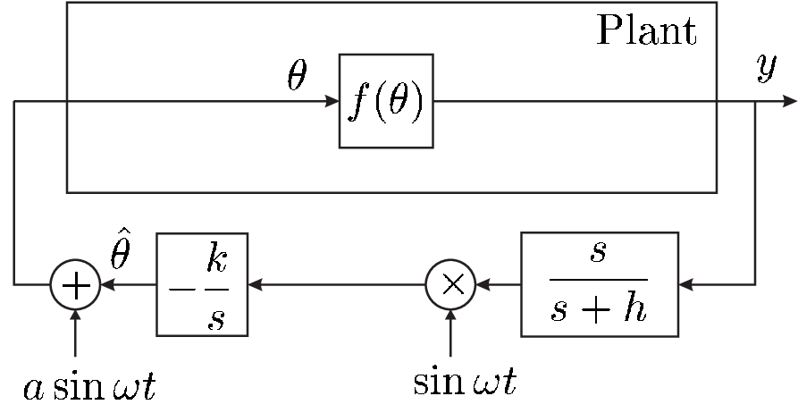
Our objective in this paper is to develop an adaptive controller that minimizes both the tracking errors and the errors in estimating the unknown parameters. Thus, we use extremum seeking as a means of optimizing a nonlinear cost function of the errors. In simple words, this cost function plays the role of the mapping $f(\theta)$ in Figure 1. This process yields an adaptation law which updates the gains of the controller. The use of a nonlinear cost function, along with the time dependent perturbation signals, lead to a non-autonomous, nonlinear set of equations. We use averaging and Lyapunov theory for stability analysis. Averaging removes time dependence from the equations and makes standard Lyapunov analysis possible. We reproduce essential definitions and theorems here for completeness and convenience.

We assume that the reader is familiar with the standard theorems regarding global asymptotic stability. Hence, we shall not provide such theorems here (see section 4.1 of [21] for example).

We are now equipped with the tools required to carry out a rigorous analysis on the use of the method of extremum seeking in adaptive control. The problem formulation and the main results are described in the following section.

To find the state tracking error dynamics, we substitute (7) and (6) into (8), and the resultant into (4). Defining the state tracking error as in (9), and the parameter convergence error as

we rearrange the resulting equation to show that the state tracking error dynamics is given by

Using Definition 3.4, we rewrite the state tracking error dynamics in state space form as

where

$\tilde{\bf a}=[\tilde{a}_{0},\ldots,\tilde{a}_{n}]^{T}$, and $\mathcal{S}$ denotes the vector of perturbation signals given by $\mathcal{S}=[c_{0}\sin\omega_{0}t,\ldots,c_{n}\sin\omega_{n}t]^{T}$. In addition, the vector $\bf v$ is the regression vector given by ${\bf v}=[y,\dot{y},\ldots,y^{(n-1)},z]^{T}$.

According to Figure 2, the parameter estimation error is governed by

Applying $s$ to the term in brackets,

where $J$ is given by (10), and $i=0,\ldots,n$. In order to write the last equation in vector form, we define a gain matrix ${\bf G}=\mbox{diag}(g_{i})\in R^{(n+1)\times(n+1)},i=0,\ldots,n+1$, and perturbation vectors, ${\bf d_{1}}(t)$ and ${\bf d_{2}}(t)$

Thus, we write (26) as

Equations (13) and (36), constitute the governing dynamics. These equations are non-autonomous since time appears explicitly in them.

Let the greatest common factor of all the probing frequencies, $\omega_{i}$,$i=0,\ldots,n$, be denoted by $\omega$. In other words, $\omega_{i}=n_{i}\omega$, where $n_{i}\in{N}$, $i=0,\ldots,n$. Furthermore, assume that $n_{i}\not=n_{j}$ for $i\not=j$. This will guarantee orthogonality of the sinusoidal perturbations. Let the design parameters be chosen such that

In order to be able to perform averaging, we scale the time as follows. Suppose that $\tau=\omega t$, and define $\varepsilon=\left(1/\omega\right)\ll 1$. By substituting $\tau=\omega t$ into (13), and using Definition 2.1, one can show that the averaged equation for tracking error dynamics is given by

Similarly, performing the same procedure on (36), one can show that the averaged equation for parameter estimation errors is given by

where $\mathcal{C}=\mbox{diag}(g_{i}d_{i}c_{i}\cos\phi_{i})\in{R}^{(n+1)\times(n+1)}$, $i=0,\ldots,n$. AppendixB provides the details on how averaging can lead us from (36) to (41).

Note that the perturbation amplitude, $c_{i}$, is chosen so as to produce a measurable variation in the plant output at the corresponding frequency.

Now, we are ready to use Lyapunov stability analysis to prove convergence of averaged tracking error, ${\bf x}_{\mbox{\scriptsize{av}}}$, to zero. Consider the following Lyapunov function

where $\bf P$, and $\bf\Gamma$ are symmetric positive definite matrices. Without loss of generality, we assume that $\varepsilon=1$, and conduct the stability analysis. We shall use the prime symbol to denote differentiation with respect to $\tau$. Taking the derivative of $V$ with respect to $\tau$ and noting that $\bf P$ and $\bf\Gamma$ are symmetric matrices, we can write

Substituting (40) and (41), and simplifying, we get

which we write as

with $Q=-({\bf A}^{T}{\bf P}+{\bf P}{\bf A})$ a positive definite matrix. By choosing the parameters in $\bf P$, $\mathcal{C}$, $\bf q$, and $\bf\Gamma$ such that

we get

that is, $V^{\prime}$ is negative semi-definite. This implies that $V(\tau)\leq V(0)$, and therefore, $\bf x_{\mbox{\scriptsize{av}}}$, and $\bf\tilde{a}_{\mbox{\scriptsize{av}}}$ are bounded. Moreover, $\bf v_{\mbox{\scriptsize{av}}}$ is also bounded by definition, since all its components are linear combinations of elements of $\bf x_{\mbox{\scriptsize{av}}}$ and the reference model. Therefore, $V^{\prime\prime}=-2{\bf x}_{\mbox{\scriptsize{av}}}^{T}{\bf QA}{\bf x}_{\mbox{\scriptsize{av}}}+\frac{2}{a_{n}}{\bf\tilde{a}}_{\mbox{\scriptsize{av}}}^{T}{\bf v}_{\mbox{\scriptsize{av}}}{\bf b}^{T}{\bf Q}{\bf x}_{\mbox{\scriptsize{av}}}$ is also bounded. Hence $V^{\prime}$ is uniformly continuous. Therefore, by Barbalat’s lemma, $V^{\prime}\to 0$ as $t\to\infty$. Hence, according to (46), ${\bf x}_{\mbox{\scriptsize{av}}}\to 0$ as $t\to\infty$, i.e. tracking error and all its derivatives converge asymptotically to zero. Furthermore, since $V\to\infty$ as $||\bf x_{\mbox{\scriptsize{av}}}||\to\infty$, global asymptotic tracking is achieved.

The following corollary, which follows from the above proof, provides some guidelines as how to choose the design parameters.

For example, we start by choosing the weighting factors $q_{i}$, and a positive definite matrix $\bf Q$, and solve for $\bf P$ using condition 4 above. Next, we choose large enough $c_{i}$’s to produce measurable variations in the plant output in the presence of noise. Then, for each parameter estimate, the gains are tuned by choosing $g_{i}$, and $d_{i}$ such that their orders of magnitude satisfy conditions 2 and 3, and their values satisfy (48) for some positive definite diagonal matrix $\Gamma$.

Since ${\bf x}_{\mbox{\scriptsize{av}}}\to 0$, therefore, $y_{\mbox{\scriptsize{av}}}\to y_{m}$ as $t\to\infty$. Using final value theorem, one can easily show that for a unit step reference signal $r(t)$, $\lim_{t\to\infty}y_{m}(t)=1/a_{m0}$. Thus, (51) will simplify to

which is the same as $k_{0}=0$.

In general, tuning the gains for optimal performance is very difficult in adaptive control, especially in MRAC. One advantage of ES-MRAC is that it provides some guidelines on gain tuning. In what follows, we shall use the results of Corollary 3.1 in a step by step manner, to help us in the process of gain tuning. Note that these steps are only provided here as guidelines, and one can use a different procedure to tune the gains. Moreover, these steps help the designer with a quick estimate of the orders of magnitudes of different gains, but will not necessarily provide optimal gains.

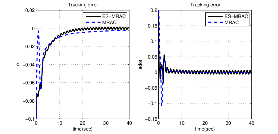
We use the following numerical values for our simulations. Let the true parameters of the system $a_{2}\ddot{y}+a_{1}\dot{y}+a_{0}y=u$, have the values $a_{2}=1$, $a_{1}=3$, and $a_{0}=6.25$. Let the model reference be given by $\ddot{y}_{m}+4.2\dot{y}_{m}+9y_{m}=r$, which corresponds to a system with a natural frequency of $\omega_{n}=3$ rad/sec and damping ratio of $\zeta=0.7$. The initial conditions are assumed to be zero for the model reference and $[y(0),\dot{y}(0)]^{T}=[-0.1,0.2]^{T}$ for the plant. The reference input $r$ is assumed to be a unit step function.

It is assumed that there is no a priori knowledge of the ideal values of parameters. Figures 3 and 4 demonstrate the performance of the system when the design parameters are chosen as follows: Let $\beta_{0}=9$, $\beta_{1}=3$, perturbation amplitudes $c_{0}=0.3$, $c_{1}=c_{2}=0.2$ perturbation frequencies $\omega_{0}=5$ rad/sec, $\omega_{1}=8$ rad/sec, $\omega_{2}=14$ rad/sec damping coefficients $d_{1}=d_{2}=d_{3}=0.1$, and gains $g_{1}=9000$, $g_{2}=3200$, $g_{3}=2000$. The matrix $\Gamma$ is chosen to be $\Gamma=0.01{\bf I_{3}}$.

We compare our results with those of MRAC applied to the same system. Definition of $\Gamma$ in chapter 8 of [10] for MRAC, is the inverse of what we have defined. Therefore, we use $\Gamma=\mbox{diag}(90,90,50)$ for MRAC. Although this is not the exact inverse of the matrix $0.01{\bf I_{3}}$, it produces better results for MRAC.

References

- [1] M. Leblanc, Sur l’electrification des chemins de fer au moyen de courants alternatifs de frequence elevee, Revue Generale de l’Electricite.
- [2] P. C. Gregory, Proceedings of the self adaptive flight control systems symposium, WADC 59-49, Wright Air Development Centre, Ohio.
- [3] H. Whitaker, J. Yamron, A. Kezer, Design of model-reference adaptive control systems for aircraft, Tech. Rep. R-16, MIT (1958).
- [4] P. V. Kokotovic, Method of sensitivity points in the investigation and optimization of linear control systems, Automat. Rem. Contr. 25 (1964) 1670–1676.
- [5] P. V. Kokotovic, B. Riedle, L. Praly, On a stability criterion for slow continuous adaptation, Syst. Control Lett. 6 (1985) 7–14.
- [6] K. J. Astrom, B. Wittenmark, Adaptive Control, 2nd Edition, Addison Wesley, Reading, MA, 1995.
- [7] K. S. Narendra, A. M. Annaswamy, Stable Adaptive Systems, Dover Publications, New York, 2005.
- [8] B. Egardt, Stability of adaptive controllers, Springer Verlag, New York, NY, 1979.
- [9] G. C. Goodwin, K. S. Sin, Adaptive Filtering Prediction and Control, Prentice-Hall, Englewood Cliffs, NJ, 1984.
- [10] J. J. E. Slotine, W. Li, Applied Nonlinear Control, Prentice Hall, New Jersey, 1991.
- [11] M. Krstic, I. Kanellakopoulos, P. V. Kokotovic, Nonlinear and Adaptive Control Design, John Wiley & Sons, New York, 1995.
- [12] P. A. Ioannou, P. V. Kokotovic, Adaptive systems with reduced models, Springer Verlag, New York, NY, 1983.
- [13] I. S. Morosanov, Method of extremum control, Automat. Rem. Contr. 18 (1957) 1077–1092.
- [14] I. I. Ostrovskii, Extremum regulation, Automat. Rem. Contr. 18 (1957) 900–907.
- [15] K. B. Ariyur, M. Krstic, Real-time optimization by extremum-seeking control, John Wiley & Sons, Hoboken, New Jersey, 2003.
- [16] K. J. Astrom, B. Wittenmark, On self-tuning regulators, Automatica 9 (1973) 185–199.
- [17] P. A. Ioannou, J. Sun, Robust Adaptive Control, Prentice Hall, New Jersey, 1995.
- [18] I. Kanellakopoulus, P. V. Kokotovic, A. S. Morse, Systematic design of adaptive controllers for feedback linearizable systems, IEEE T. Automat. Contr. 36 (1991) 1241–1253.
- [19] I. Kanellakopoulus, P. V. Kokotovic, A. S. Morse, Adaptive feedback linearization of nonlinear systems, in: Foundations of Adaptive Control, Springer-Verlag, Berlin, 1991, pp. 311–346.
- [20] P. Haghi, K. B. Ariyur, On the extremum seeking of model reference adaptive control in higher-dimensional systems, in: Proc. 2011 Amer. Contr. Conf., San Francisco, California, 2011, pp. 1176–1181.
- [21] H. K. Khalil, Nonlinear Systems, 3rd Edition, Prentice Hall, New Jersey, 2002.
- [22] K. B. Ariyur, S. Ganguli, D. F. Enns, Extremum seeking for model reference adaptive control, in: Proc. of the AIAA Guidance, Navigation, and Control Conference, Chicago, Illinois, 2009.
A Proof of Theorem 3.3
Proof 3
In order to study the properties of the actual system, we note that we can write the governing equations of the system, as . That is, (13) and (36) can be written as , with , and
As shown in section 3, we scale the time using , with , and . Thus we get