Studies in Astronomical Time Series Analysis.
VI. Bayesian Block Representations
Jeffrey D. Scargle
Space Science and Astrobiology Division,
NASA Ames Research Center
Jay P. Norris
Physics Department, Boise State University
Brad Jackson
San José State University, Department of Mathematics and Computer Science,
The Center for Applied Mathematics and Computer Science
James Chiang
Kavli Institute, SLAC
Keywords: time series, signal detection, triggers, transients, Bayesian analysis
“The line is similar to a length of time, and as the points are the beginning and end of the line, so the instants are the endpoints of any given extension of time.” Leonardo da Vinci, Codex Arundel, folio 190v., c. 1500 A.D. [Capra 2007].
Abstract
This paper addresses the problem of detecting and characterizing local variability in time series and other forms of sequential data. The goal is to identify and characterize statistically significant variations, at the same time suppressing the inevitable corrupting observational errors. We present a simple nonparametric modeling technique and an algorithm implementing it—an improved and generalized version of Bayesian Blocks [Scargle 1998]—that finds the optimal segmentation of the data in the observation interval. The structure of the algorithm allows it to be used in either a real-time trigger mode, or a retrospective mode. Maximum likelihood or marginal posterior functions to measure model fitness are presented for events, binned counts, and measurements at arbitrary times with known error distributions. Problems addressed include those connected with data gaps, variable exposure, extension to piecewise linear and piecewise exponential representations, multi-variate time series data, analysis of variance, data on the circle, other data modes, and dispersed data. Simulations provide evidence that the detection efficiency for weak signals is close to a theoretical asymptotic limit derived by [Arias-Castro, Donoho and Huo 2003]. In the spirit of Reproducible Research [Donoho et al. (2008)] all of the code and data necessary to reproduce all of the figures in this paper are included as auxiliary material.
1 The Data Analysis Setting
This paper describes a method for nonparametric analysis of time series data to detect and characterize structure localized in time. Nonparametric methods seek generic representations, in contrast to fitting of models to the data. By local structure we mean light-curve features occupying sub-ranges of the total observation interval, in contrast to global signals present all or most of the time (e.g. periodicities) for which Fourier, wavelet, or other transform methods are more appropriate. The goal is to separate statistically significant features from the ever-present random observational errors. Although phrased in the time-domain the discussion throughout is applicable to measurements sequential in wavelength, spatial quantities, or any other other independent variable.
This setting leads to the following desiderata: The ideal algorithm would impose as few preconditions as possible, avoiding assumptions about smoothness or shape of the signal that place a priori limitations on scales and resolution. The algorithm should handle arbitrary sampling (i.e., not be limited to gapless, evenly spaced data) and large dynamic ranges in amplitude, time scale and signal-to-noise. For scientific data mining applications and for objectivity, the method should be largely automatic. To the extent possible it should suppress observational errors while preserving whatever valid information lies in the data. It should be applicable to multivariate problems. It should incorporate variation of the exposure or instrumental efficiency during the measurement, as well auxiliary, extrinsic information, e.g. spectral or color information. It should be able to operate both retrospectively (analyze all the data after they are collected) and in a real-time fashion that triggers on the first significant variation of the signal from its background level.
The algorithm described here achieves considerable success in each of these desired features. In a simple and easy-to-use computational framework it represents the structure in the signal in a form handy for further analysis and the estimation of physically meaningful quantities. It includes an automatic penalty for model complexity, thus solving the vexing problems associated with model comparison in general and determining the order of the model in particular. It is exact, not a greedy11 1 This term refers to algorithms that greedily make optimal improvements at each iteration but are not guaranteed to converge to a globally optimal solution. approximation as in [Scargle 1998].
Versions of this algorithm have been used in various applications, such as [Qin et al. 2012, Norris Gehrels and Scargle 2010, Norris Gehrels and Scargle 2011, Way Gazis and Scargle 2011].
The following sections discuss, in turn, the basis of segmentation analysis (§1.1), the piecewise constant model adopted in this work (§1.2), extensions to piecewise linear and piecewise exponential models (§1.3), the types of data that the algorithm can accept (§§1.5 and 1.6), data gaps (§1.7), exposure variations (§1.8), a parameter from the prior on the number of blocks (§1.9), generalities of optimal segmentation of data into blocks (§2), some error analysis (§2.8), a variety of block fitness functions (§3), and sample applications (§4). Appendices present some MatLab © code, some miscellaneous results, and details of other data modes, including dispersed data (§C.8). Ancillary files are available providing scripts and data in order to reproduce all of the figures in this paper.
1.1 Optimal Segmentation Analysis
The above considerations point toward the most generic possible nonparametric data model, and have motivated the development of data segmentation and change-point methods – see e.g. [Ò Ruanaidh and Fitzgerald 1996, Scargle 1998]. These methods represent the signal structure in terms of a segmentation of the time interval into blocks, with each block containing consecutive data elements satisfying some well defined criterion. The optimal segmentation is that which maximizes some quantitative expression of the criterion – for example the sum over blocks of a goodness-of-fit of a simple model of the data lying in each block.
These concepts and methods can be applied in surprisingly general, higher dimensional contexts. Here, however, we concentrate on one-dimensional data ordered sequentially with respect to time or some other independent variable. In this setting segmentation analysis is often called change-point detection, since it implements models in which a signal’s statistical properties change discontinuously at discrete times but are constant in the segments between these change-points (see §2.5).
1.2 The Piecewise Constant Model
It is remarkable that all of the desiderata outlined in the previous section can be achieved in large degree by optimal fitting of a piecewise-constant model to the data. The range of the independent variable (e.g. time) is divided into subintervals (here called blocks) generally unequal in size, in which the dependent variable (e.g. intensity) is modeled as constant within errors. Of all possible such “step-functions” this approach yields the best one by maximizing some goodness-of-fit measure.
Defining the times ending one block and starting the next as change-points, the model of the whole observation interval contains these parameters:
- (1)
-
: the number of change-points
- (2)
-
: the change-point starting block
- (3)
-
: the signal amplitude in block
for .22 2 There is one more block than there are change-points: The first datum is always considered a change-point, marking the start of the first block, and is therefore not a free parameter. If the last datum is a change-point, it denotes a block consisting solely of that datum. The key idea is that the blocks can be treated independently, in the sense that a block’s fitness depends on its data only. Our simple model for each block has effectively two parameters. The first represents the signal amplitude, and is treated as a nuisance parameter to be determined after the change-points have been located. The second parameter is the length of the interval spanned by the block. (The actual start and stop times of this interval are needed for piecing blocks together to form the final signal representation, but not for the fitness calculation.)
How many blocks? A key issue is how to determine the number of blocks, . Nonparametric analysis invariably involves controlling in one way or another the complexity of the estimated representation. Typically such regulation is considered a trade-off of bias and variance, often implemented by adjusting a smoothing parameter.
But smoothing is one of the very things we are trying to avoid. The discontinuities at the block edges are regarded as assets, not liabilities to be smoothed over. So rather than smooth we influence the number of blocks by defining a prior distribution for the number of blocks. Adjusting a parameter controlling the steepness of this prior establishes relative probabilities of smaller or larger numbers of blocks. In the usual fashion for Bayesian model selection in cases with high signal-to-noise is determined by the structure of the signal; with lower signal-to-noise the prior becomes more and more important. In short, we are regulating not smoothness but complexity, much in the way that wavelet denoising [Donoho and Johnstone 1998] operates without smoothing over sharp features as long as they are supported by the data. The adopted prior and the determination of its parameter are discussed in §1.9 below.
This segmented representation is in the spirit of nonparametric approximation and not meant to imply that we believe the signal is actually discontinuous. The sometimes crude and blocky appearance of this model may be awkward in visualization contexts, but for deriving physically meaningful quantities it is not. Blocky models are broadly useful in signal processing [Donoho 1994] and have several motivations. Their simplicity allows exact treatment of various quantities, such as the likelihood. We can optimize or marginalize the rate parameters exactly, giving simple formulas for the fitness function (see §3 and Appendix C,§C). And in many applications the estimated model itself is less important than quantities derived from it. For example, while smoothed plots of pulses within gamma-ray bursts make pretty pictures, one is really interested in pulse locations, lags, amplitudes, widths, rise and decay times, etc. All these quantities can be determined directly from the locations, heights and widths of the blocks – accurately and free of any smoothness assumptions.
1.3 Piecewise Linear and Exponential Models
Some researchers have applied segmentation methods with other block representations. For example piecewise linear models have been used in measuring similarity among time series and in pattern matching [Lin, Keogh, Lonardi and Chiu 2003] and to represent time series generated by non-linear processes [Tong 1990]. While such models may seem better than discontinuous step functions, their improved flexibility is somewhat offset by added complexity of the model and its interpretation. Note further that if continuity is imposed at the change-points, a piecewise linear model has essentially the same number of degrees of freedom as does the simpler piecewise constant model.
We mention two such generalizations, one modeling the signal as linear in time across the block:
| (1) |
and the second as exponential:
| (2) |
In both cases is the signal strength at the fiducial time and the coefficient determines the rate of variation over the block. Such models may be useful in spite of the caveats mentioned above and the added complexity of the block fitness functions. Hence we provide some details in Appendix C, §§C.9 and C.10.
1.4 Histograms
For event data
the piecewise constant representation
can be interpreted as
a histogram of the measured
values – one in which the bins
are not fixed ahead of time and
are free to be unequal in size
as determined by the data.
In this context the time order
of the measurements is irrelevant.
Once one determines
the parameter in the prior
on the number of bins, ncp_prior,
one has an objective histogram procedure
in which the number,
individual sizes, and
locations of the bins
are determined solely and uniquely by the data.
1.5 Data Modes
The algorithms developed here can be used with a variety of types of data, often called data modes in instrumentation contexts. An earlier paper [Scargle 1998] described several, with formulas for the corresponding fitness functions. Here we discuss data modes in a broader perspective. It is required that the measurements provide sufficient information to determine which block they belong to and then to compute the model fitness function for the block (cf. §2.3).
Almost any physical variable and any measurement scheme for it, discrete or quasi-continuous, can be accommodated. In the simple one dimensional case treated here, the independent variable is time, wavelength, or some other quantity. The data space is the domain of this variable over which measurements were made – typically an interval, possibly interrupted by gaps during which the measuring system was not operating.
The measured quantity can be almost anything that yields information about the target signal. The three most common examples emphasized here are: (a) times of events (often called time-tagged event data, or TTE), (b) counts of events in time bins, and (c) measurements of a quasi-continuous observable at a sequence of points in time. For the first two cases the signal of interest is the event rate, proportional to the probability distribution regulating events which occur at discrete times due to the nature of the astrophysical process and/or the way it is recorded. We call case (c) point measurements, not to be confused with point data (also called event data). These modes have much in common, as they all comprise measurements that can be at any time; what differentiates them is their statistics, roughly speaking Bernoulli, Poisson, and Gaussian (or perhaps some other) respectively.
The archetypal example of (a) is light collected by a telescope and recorded as a set of detection times of individual photons to study source variability. Case (b) is similar, but with the events collected into bins – which do not have to be equal or evenly spaced. Case (c) is common when photons are not detected individually, such as in radio flux measurements. In all cases it is useful to represent the measurements with data cells, typically one for each measurement (see §2.2). In principle mixtures of cells from different data types can be handled, as described in the next section.
1.6 Mixed Data Modes
Our algorithm can analyze mixtures of any data types within a single time series. For example the data stream could consist of arbitrary combinations of cells of the three types defined above – measured values, counts in bins and events – with or without overlap in time among the various data modes. In regions of overlap the block representation would be based on the combined data; otherwise it would represent block structures supported by the corresponding individual data modes. In such applications the cost function must refer to a common signal amplitude parameter, possibly including normalization factors to account for differences in the measurement processes.
A related concept is that of multivariate time series, usually referring to concurrent observations from different telescopes. The distinction between this concept and mixed data modes is largely semantic. Hence we leave implimentation details to §4.2.
1.7 Gaps
In some cases there are subintervals over which no data can be obtained. For example there may be random interruptions such as detector malfunction at unpredictable but known periods of time, or regular interruptions as the Earth periodically blocks the view of an object from an orbiting space observatory. (Of course this case is very different from intervals in which no events happened to be detected, due to low event rate, or in which one simply did not happen to make point measurements.
Such data gaps have a nearly invisible affect on the algorithm, fundamentally due to the fact that it operates locally in the time domain. For event data all that matters is the live time during the block, i.e. the time over which data could have been registered. Other than correcting the total time span of any putative block containing data gaps by subtracting the corresponding dead time, gaps can be handled by ignoring them. Operationally one simply treats the data right after a gap as immediately following the data right before it (and not delayed by the length of the gap). Think of this as squeezing the interval to eliminate the gaps, carrying out the analysis as if no gaps are present, and then un-doing the squeezing by restoring the original times. This procedure is valid because event independence means that the fitness of a block depends on only its total live-time and the events within it.
For event data this squeezing can be implemented by subtracting from each event time the sum of the lengths of all the preceding gaps. One small detail concerns the points just before and just after a gap. One might think their time intervals should be computed relative to the gap edges. But it follows from the nature of independent events (Appendix B, §B) that they can be computed as though the gap did not exist.
The only other subtlety lies in interpreting the model in and around gaps. There are two possibilities: a given gap (a) may lie completely within a block or (b) it may separate two blocks. Case (a) can be taken as evidence that the event rates before and after the gap are deemed the same within statistical fluctuations. Case (b) on the other hand implies that the event rate did change significantly.
Of course the gaps must be restored for display and other post-processing analysis. Think of this as un-squeezing the data so that all blocks appear at their correct locations in time. Keeping in mind that there is no direct information about what happened during unobserved intervals, plots should probably include some indication that rates within gaps are unknown or uncertain, such as by use of dotted lines or shading in the gap for case (a) or leaving the gap interval completely blank in case (b).
For the case of point measurements the situation is different. In one sense there are no gaps at all, and in another sense the entire observation interval consists of many gaps separating tiny intervals over which the measurements were actually made. One is hard-pressed to make a statistical distinction between various reasons why there is not a measurement at a given time – e.g. detector and weather problems, or simply a choice as to how to allocate observing time (a choice that may even depend on the results of analyzing previous data). Basically the blocks in this case represent intervals where whatever measurements were made in the interval are consistent with a signal that is constant over that interval.
Note that things would be different if one wanted to define a fitness function dependent on the total length of the block, not just its live time. This would arise for example if a prior on the block length were imposed. Such possibilities will not be discussed here.
1.8 Exposure Variations
In some applications the effective instrument response is not constant. The measurements then reflect true source variations modified by changes in overall throughput of the detection system. We use the term exposure for any such effect on the detected signal – e.g. detector efficiency, telescope effective area, beam pattern and point spread function effects. Exposure can be quantified by the ratio of the expected signal with and without any such effects. It may be calculable from properties of the observing system, determined after the fact through some sort of calibration procedure, or a combination of the two. Here we assume that this ratio is known and expressed as a number , typically with , for data cell .
The adjustment for exposure is simple, namely change the parameter representing the observed signal amplitude in the likelihood to what it would have been if the exposure had been unity. First compute the exposure for data cell . Then increase by the factor whatever quantity in the data cell represents the measured signal intensity. Specifically, for time-tagged event data this parameter is the reciprocal of the interval of the corresponding data cell: (see eq. (20)), which is then replaced with . For bin counts the bin size can be multiplied by or equivalently the count by . For point measurements multiply the amplitude measurement by (and adjust any observational error parameters accordingly). In all cases the goal is to represent the data as closely as possible to what it would have been if the exposure had been constant. Of course this restoration is not exact in individual cases, but is correct on average.
For TTE data the fact that interval as we define it in eq. (20) depends on the times of two different events (just previous to and just after the one under consideration) may seem to pose a problem. The exposures of these events will in general be different, so what value do we use for the given event? The comforting answer is that the only relevant exposure is that for the given event itself. For consider the interval from the previous to the current time, namely . Here is regarded as simply a fiducial time and the distribution of this interval is given by eq. (47) with the true rate adjusted by the exposure for event , by the principle described in §B.5 just after this equation. Similarly by a time-reversal invariance argument the distribution of the interval to the subsequent event, namely , also depends on only the same quantity. In summary event independence (Appendix C, §C) yields the somewhat counterintuitive fact that the probability distribution of of the interval surrounding event depends on only the effective event rate for event .
1.9 Prior for the Number of Blocks
Earlier work [Scargle 1998] did not assign an explicit prior probability distribution for the number of blocks, i.e. the parameter . This omission amounts to using a flat prior, but in many contexts it is unreasonable to assign the same prior probability to all values. In particular, in most settings it is much more likely a priori that than that . For this reason it is desirable to impose a prior that assigns smaller probability to a large number of blocks, and we adopt this geometric prior [Coram 2002]:
| (3) |
for , and zero otherwise since cannot be negative or larger than the number of data cells. The normalization constant is easily obtained, giving
| (4) |
Through this prior the parameter influences the number of blocks in the optimal representation – a number of some importance since it affects the visual appearance of the representation and to a lesser extent the values of quantities derived from it. This form for the distribution dictates that finding blocks is less likely by the constant factor than is finding blocks. In almost all applications will be chosen to express that a smaller number of blocks is a priori more likely than a larger number.
In principle the choice of a prior and the values of its parameters expresses one’s prior knowledge in a specific problem. The convenient geometric prior adopted here has proven to be generic and flexible, and its parameterization is simple and straightforward. These properties are appropriate for a generic analysis tool meant for a wide variety of applications. One can think of selecting as a simple way of adjusting the amount of structure in the block representation of the signal. It is specifically not a smoothing parameter but is analogous to one.
The expected number of blocks follows from eq. (3)
| (5) |
Note that the actual number of blocks is a discontinuous, monotonic function of , and because its jumps can be it is not generally possible to force a prescribed number by adjusting this parameter.
The above prior is not the only one possible
and different forms may be useful in some applications.
But Eq. (3) is very convenient to implement,
since with the fitness equal to the
log of the posterior, one only needs to subtract the constant
(called ncp_prior in the MatLab code
and in the discussion of computational issues
below)
from the fitness of each block.
Determining the value
to use in applications is
discussed in §2.7 below.
2 Optimum Segmentation of Data on an Interval
Piecewise constant modeling of sequential measurements on a time interval is most conveniently implemented by seeking an optimal partition of the ordered set of data cells within . In this special case of segmentation the segments cover the whole set with no overlap between them (Appendix B). Segmentations with overlap are possible, for example in the case of correlated measurements, but are not considered here. One can envision our quest for the optimal segmentation as nothing more than finding the best step-function, or piecewise constant model, fit to the data – defined by maximizing a specific fitness measure as detailed in §2.4.
We introduce our algorithm in a somewhat abstract setting because the formalism developed here applies to other data analysis problems beyond time series analysis. It implements Bayesian Blocks or other 1D segmentation ideas for any model fitness function that satisfies a simple additivity condition. It improves the previous approximate segmentation algorithm [Scargle 1998] by achieving an exact, rigorous solution of the multiple change-point problem, guaranteed to be a global optimum, not just a local one.
The rest of this section describes how the model is structured for effective solution of this problem, while details on the quantity to be optimized are deferred to the next section.
2.1 Partitions
Partitions of a time interval are simply collections of non-overlapping blocks (defined below in §2.3), defined by specifying the number of its blocks and the block edges:
| (6) |
where the are indices of the data cells (§2.2) defining times called change-points (see §2.5).
Appendix B gives a few mathematical details about partitions, including justification of the restriction of the change-points to coincide with data points and the result that the number of possible partitions (i.e. the number of ways cells can be arranged in blocks) is . This number is exponentially large, rendering an explicit exhaustive search of partition space utterly impossible for all but very small . Our algorithm implicitly performs a complete search of this space in time of order , and is practical even for , for which approximately partitions are possible. The beauty of the algorithm is that it finds the optimum among all partitions without an exhaustive explicit search, which is obviously impossible for almost any value of arising in practice.
2.2 Data Cells
For input to the algorithm the measurements are represented with data cells. For the most part there is one cell for each measurement, although in the case of TTE data two or more events with identical time-tags may be combined into a single cell. A convenient data structure is an array containing the cells ordered by the measurement times.
Specification of the contents of the cells must meet two requirements. First they must include time information allowing determination of which cells lie in a block given its start and stop times. Post-processing steps such as plotting the blocks may in addition use the actual times, either absolute or relative to a specified origin.
The other requirement is that the fitness of a block can be computed from the contents of all the cells in it (§2.4, §3). For the three standard cases the relevant data are roughly speaking: (a) intervals between events (§3.1), (b) bin sizes, locations and counts (§3.2), and (c) measured values augmented by a quantifier of measurement uncertainty (§3.3). These same quantities enable construction of the resulting step function for post-processing steps such as computing signal parameters.
2.3 Blocks of Cells
A block is any set of consecutive cells, either an element of the optimal representation or a candidate for it. Each block represents a subinterval (within the full range of observation times) over which the amplitude of the signal can be estimated from the contents of its cells (§2.2). A block can be as small as one cell or as large as all of the cells.
Our time series model consists of a set of blocks partitioning the observations. All model parameters are constant within each block but undergo discrete jumps at the change-points (§2.5) marking the edges of the blocks. The model is visualized by plotting rectangles spanning the intervals covered by the blocks, each with height equal to the signal intensity averaged over the interval. The concept of fitness of a block is fundamental to everything else in this paper. As we will see in the next section the fitness of a partition is the sum of the fitnesses of the blocks comprising it.
2.4 Fitness of Blocks and Partitions
Since the goal is to represent the data as well as possible within a given class of models, we maximize a quantity measuring the fitness of models in the given class, here the class of all piecewise constant models. Alternatively, one can minimize an error measure. Both operations are called optimization. The algorithm relies on the fitness being block-additive, i.e.
| (7) |
where is the total fitness of the partition P of interval , and is the fitness of block . The latter can be any convenient measure of how well a constant signal represents the data within the block. Typically additivity results from independence of the observational errors. We here ignore the possibility of correlated errors, which could make the fitness of one block depend on that of its neighbors. Remember correlation of observational errors is quite separate from correlations in the signal itself.
All model parameters are marginalized except the specifying block edges. Then the total fitness depends on only these remaining parameters – i.e. on the detailed specification of the partition by indicating which cells fall in each of its blocks. The best model is found by maximizing over all possible such partitions.
2.5 Change-points
In the time series literature a point at which a statistical model undergoes an abrupt transition, by one or more of its parameters jumping instantaneously to a new value, is called a change-point. This is exactly what happens at the edges of the blocks in our model. In principle change-points can be at arbitrary times. However, following the data cell representation and without any essential loss of generality they can be restricted to coincide with a data point (Appendix B; §B).
A few comments on notation are in order. We take blocks to start at the data cell identified by the algorithm as a change-point and to end at the cell previous to the subsequent change-point. A slight variation of this convention is discussed below in §4.4 in connection with allowing the possibility of empty blocks in the context of event data. One might adopt other conventions, such as apportioning the change-point data cell to both blocks, but we do not do so here. Even though the first data cell in the time series always starts the first block, our convention is that it is not considered a change-point. In the code presented here the first change-point marks the start of the second block. For the -th block starts at index and ends at . The first block always starts with the very first data cell. The last block always terminates with the very last data cell. If the last cell is a change-point, it defines a block consisting of only that one cell. The set of change-points is empty if the best model consists of a single block, meaning that the time series is sensibly constant over the whole observation interval. The number of blocks is one greater than the number of change-points.
2.6 The Algorithm
We now outline the basic algorithm yielding the desired optimum partitions. The details of this dynamic programming33 3 Bellman’s explanation (before the word “programming” took on its current computational connotation) of how he chose this name is interesting. The Secretary of Defense at the time “… had a pathological fear and hatred of the word, research. … You can imagine how he felt, then, about the term, mathematical. … I felt I had to do something to shield … the Air Force from the fact that I was really doing mathematics inside the RAND Corporation. … I was interested in planning … But planning is not a good word for various reasons. I decided therefore to use the word, Ôprogramming.Õ I wanted to get across the idea that this was dynamic … it’s impossible to use the word, dynamic, in a pejorative sense. Try thinking of some combination that will possibly give it a pejorative meaning. It’s impossible. Thus, I thought dynamic programming was a good name. It was something not even a Congressman could object to. approach [Bellman 1961, Hubert, Arabie, and Meulman 2001, Dreyfus 2002] are in [Jackson et al. 2005]. It follows the spirit of mathematical induction: beginning with the first data cell, at each step one more cell is added. The analysis makes use of results stored from all previous steps. Remarkably the algorithm is exact and yields the optimal partition of an exponentially large space in time of order . The iterations normally continue until the whole interval has been analyzed. However its recursive nature allows the algorithm to function in a trigger mode, halting when the first change-point is detected (§4.3).
Let denote the optimal partition of the first cells. In the starting case the only possible partition (one block consisting of the first cell by itself) is trivially optimal. Now assume we have completed step , identifying the optimal partition . At this (and each previous) step store the value of optimal fitness itself in array best and the location of the last change-point of the optimal partition in array last.
It remains to show how to obtain . For some consider the set of all partitions (of these first cells) whose last block starts with cell (and by definition ends at ). Denote the fitness of this last block by . By the subpartition result in Appendix B the only member of this set that could possibly be optimal is that consisting of followed by this last block. By the additivity in Eq. (7) the fitness of said partition is the sum of and the fitness of saved from a previous step:
| (8) |
is the special case where the last block comprises the entire data array and thus no previous fitness value is needed. Over the indicated range of this equation expresses the fitness of all partitions P(R+1) that can possibly be optimal. Hence the value of yielding the optimal partition is the easily computed value maximizing :
| (9) |
At the end of this computation, when , it only remains to find the locations of the change-points of the optimal partition. The needed information is contained in the array last in which we have stored the index at each step. Using the corollary in Appendix B it is a simple matter to use the last value in this array to determine the last change-point in , peel off the end section of last corresponding to this last block, and repeat. That is to say, the set of values
| (10) |
are the index values giving the locations of the change-points, in reverse order. Note that the positions of the change-points are not necessarily fixed until the very last iteration, although in practice it turns out that they become more or less ‘‘frozen’’ once a few succeeding change-points have been detected. MatLab44 4 ™The Mathworks, Inc code for optimal partitioning of event data is given in Appendix A.
2.7 Fixing the Parameter in the Prior Distribution for
As mentioned in §1.9 the output of the algorithm is dependent on value of the parameter , characterizing the assumed prior distribution for the number of blocks, eq. (3). In many applications the results are rather insensitive to the value as long as the signal-to-noise ratio is even moderately large. Nevertheless extreme values of this parameter give bad results in the form of clearly too few or too many blocks. In any case one must select a value to use in applications.
This situation is much like that of selecting a smoothing parameter in various data analysis applications, e.g. density estimation. In such contexts there is no perfect choice but instead a tradeoff between bias and variance. Here the tradeoff is between a conservative choice not fooled by noise fluctuations but potentially missing real changes, and a liberal choice better capturing changes but yielding some false detections. Several approaches have proven useful in elucidating this tradeoff. Merely running the algorithm with a few different values can indicate a range over which the block representation is reasonable and not very sensitive to the parameter value (cf. Fig. 1).
The discussion of fitness functions below
in §3
gives implementation details of
an objective
method for calibrating ncp_prior
as a function of the number of data points.
It is based on
relating this parameter
to the false positive probability –
that is, the relative frequency with which
the algorithm falsely reports detection of
a change-point in data with no signal present.
It is convenient to use the complementary quantity
| (11) |
This number is the frequency with which the algorithm
correctly rejects the presence of a change-point
in pure noise.
Therefore it is also the probability that a
change-point reported by the algorithm
with this value of ncp_prior
is indeed statistically significant –
hence we call it the
correct detection rate for single change-points.
The needed
ncp_prior-
relationship is easily found by noting that
the rates of correct and incorrect responses to
fluctuations in simulated pure noise can be controlled by
adjusting the value of ncp_prior.
The procedure is:
generate a synthetic pure-noise time series;
apply the algorithm for a range of ncp_prior;
select the smallest value
that yields false detection frequency
equal or less than the desired rate, such as .05.
The values of ncp_prior
determined in this way are
averaged over a large number of realizations
of the random data.
The result depends on only the number
of data points and the adopted value of :
| (12) |
Results from simulations of this kind are given below for the various fitness functions in §§3.1, 3.2, and 3.3. We have no exact formulas, but rather fits to these numerical simulations.
The above discussion is useful in
the simple problem of deciding
whether or not a signal
is present above a background of noisy
observations.
In other words we have a procedure for
assigning a value of ncp_prior
that results in an acceptable frequency of
spurious change-points, or false positives,
when searching for a single statistically significant change.
Real-time triggering on transients
(§4.3) is an example of this situation,
as is any case where
detection of a single change-point
is the only issue in play.
But elucidating the shape of an actual detected signal
lies outside the scope of the above procedure,
since it is based on a pure noise model.
A more general goal
is to limit the number of both false negatives and
false positives in the context of an extended signal.
The choice of the parameter value here
depends on the nature of the signal
present and the signal-to-noise level.
One expects that somewhat larger values of
ncp_prior are necessary
to guard against corruption of the
estimate of the signal’s shape
due to errors at multiple change-points.
This idea suggests
a simple extension of the above procedure.
Assume that a value of
, the probability of correct detection
of an individual change-point,
has been adopted and the corresponding
value of ncp_prior
determined
with pure noise simulations as outlined above
and expressed in eq. (12).
For a complex signal our goal is
correct detection of not just one, but
several change-points, say in number.
The trick is to treat each of them
as an independent
detection of a single change-point
with success rate .
The probability of all successes
follows
from the law of compound probabilities:
| (13) |
There are problems with this analysis in that the following are not true:
-
(1) Change-point detection in pure noise and in a signal are the same.
-
(2) The detections are independent of each other.
-
(3) We know the value of .
All of these statements would have to be true
for eq. (13) to be rigorously valid.
We propose to regard the first
two as approximately true and address the
third as follows:
Decide that the probability of correctly detecting all the
change-points should be
at least a high as some value ,
such as .
Apply the algorithm using the value of
ncp_prior =
given by the pure noise simulation.
Use eq. (13) and
the number of change-points thus found to yield
a revised value
| (14) |
Stopping when
the iteration produces
no further modification of
the set of change-points,
one has the
recommended value of ncp_prior.
This ad hoc procedure is not rigorous, but it establishes
a kind of consistency and has proven useful
in all the cases where we have tried it,
e.g. [Norris Gehrels and Scargle 2010, Norris Gehrels and Scargle 2011].

Fig. 1 shows another approach, based on
cross-validation of the data being analyzed
(cf. [Hogg 2008]).
This study uses the collection of
raw TTE data at the BATSE web site
ftp://legacy.gsfc.nasa.gov/compton/data/batse/ascii_data/batse_tte/.
The files for each of 532 GRBs
contain time tags for all photons
detected for that burst.
The energy and
detector tags in the data files were not used here,
but §4.1 shows an example using the former.
An ordinary 256-bin histogram of
all photon times for each of 532 GRBs
was taken as the true signal for that burst.
Eight random subsamples smaller by a factor of were
analyzed with the algorithm
using the fitness in eq. (19).
The average RMS error between
these block representations
(evaluated at the same 256 time points)
and the histogram is roughly flat over a
broad range.
While this illustration with
a relatively homogeneous data set
should obviously not be taken as universal,
the general behavior seen here – determination
of a broad range of nearly equally optimal
values of ncp_prior –
is characteristic of a wide variety of situations.
2.8 Analysis of Variance
Assessment of uncertainty is an important part of any data analysis procedure. The observational errors discussed throughout this paper are propagated by the algorithm to yield corresponding uncertainties in the block representation and its parameters. The propagation of stochastic variability in the astronomical source is a separate issue, called cosmic variance, and is not discussed here.
Since the results here comprise a complete function defined by a variable number of parameters, quantification of uncertainty is considerably more intricate than for a single parameter. In particular one must specify precisely which of the block representation’s aspects is at issue. Here we discuss three: (a) the full block representation, (b) the very presence of the change-points themselves, and (c) locations of change-points.
A straightforward way to deal with (a) is by bootstrap analysis. As described in [Efron and Tibshirani 1998] for time series data this procedure is rather complicated in general. However resampling of event data in the manner appropriate to the bootstrap is trivial. The procedure is to run the algorithm on each of many bootstrap samples and evaluate the resulting block representations at a common set of evenly spaced times. In this way models with different numbers and locations of change-points can be added, yielding means and variances for the estimated block light curves. The bootstrap variance is an indicator of light curve uncertainty. In addition comparison of the bootstrap mean with the block representation from the actual data adds information about modeling bias. The former is rather like a model average in the Bayesian context. This average typically smoothes out the discontinuous block edges present in any one representation. In some applications the bootstrap mean may be more useful than the block representation.
This method does not seem to be useful for studying uncertainty in the change-points themselves, in particular their number, presumably because the duplication of data points due to the replacement feature of the resampling yields excess blocks (but with random locations and small amplitude variance, and therefore with little effect on the mean light curve).
By (b) is meant an assessment of the
statistical significance of the identification
of a given change point.
For a given change-point
we suggest quantification of this uncertainty
by evaluating the ratio of the fitness functions
for the two blocks on either side of that change-point
to that of the
single block that would exist if the
change-point were not there.
The corresponding difference of the (logarithmic)
fitness values should be adjusted by the
value of the constant parameter ncp_prior,
for consistency with the way fitness is computed
in the algorithm.
Finally, (c) is easily addressed in an approximate way by fixing all but one change-point and computing fitness as a function of the location of that change-point. This assessment is approximate because by fixing the other change-points because it ignores inter-change-point dependences. One then converts the run of the fitness function with change-point location into a normalized probability distribution, giving comprehensive statistical information about that location (mean, variance, confidence interval, etc.)
2.9 Multivariate Time Series
Our algorithm’s intentionally flexible data interface not only allows processing a wide variety of data modes but also facilitates joint analysis of mode combinations. This feature allows one to obtain the optimal block representation of several concurrent data streams with arbitrary modes and sample times. This analysis is joint in the sense that the change-points are constrained to be at the same times for all the input series; in other words the block edges for all of the input data series line up. The representation is optimal for the data as a whole but not for the individual time series.
To interpret the result of a multivariate analysis one can study the blocks in the different series in two ways: (a) separately, but with the realization that the locations of their edges are determined by all the data; or (b) in a combined representation. The latter requires that there be a meaningful way to combine amplitudes. For example the plot of a joint analysis of event and binned data could simply display the combined event rate for each block, perhaps adjusting for exposure differences. For other modes, such as photon events and radio frequency fluxes, a joint display would have to involve a spectral model or some sort of relative normalization. The example in §4.2 below will help clarify these issues.
The idea extending the basic algorithm to incorporate multiple time series is simple. Each datum in any mode has a time-tag associated with it – for example the event time, the time of a bin center, or the time of a point measurement. The joint change-points are allowed to occur at any one of these times. Hence the times from all of the separate data streams are collected together into a single ordered array; the ordering means that the times – as well as the measurement data – from the different modes are interleaved.

The cartoon in Fig. 2 shows how the individual concatenated times and data series are placed in separate blocks in a matrix (top) and then redistributed (bottom) by ordering the combined times. Then the fitness function for a given data series can be obtained from the corresponding data slice (e.g. the horizontal dashed line in the figure, for Series #2). The zero entries in these slices (indicated by white space in the figure) are such that the fitness function for data from each series is evaluated for only the appropriate data and mode combination. The overall fitness is then simply the sum of those for the several data series. The details of this procedure are described in the code provided in Appendix A (§A).
2.10 Comparison with Theoretical Optimal Detection Efficiency
How good is the algorithm at extracting weak signals in noisy data? This section gives evidence that it achieves detection sensitivity closely approaching ideal theoretical limits. The formalism in [Arias-Castro, Donoho and Huo 2003] treats detection of geometric objects in data spaces of arbitrary dimension using multiscale methods. The one dimensional special case in §II of this reference is essentially equivalent to our problem of detecting a single block in noisy time series.
Given measurements normalized so that the observational errors (normally distributed with zero mean and variance ), these authors show that the threshold for detection is
| (15) |
This result is asymptotic (i.e. valid in the limit of large ). It is valid for a frequentist detection strategy based on testing whether the maximum of the inner product of the model with the data exceeds the quantity in eq. (15) or not. These authors state “In short, we can efficiently and reliably detect intervals of amplitude roughly , but not smaller.” More formally the result is that asymptotically their test is powerful for signals of amplitude greater than and powerless for weaker signals.

It is of interest to see how well our algorithm stacks up against these theoretical results, since the two analysis approaches (matched filter test statistic vs. Bayesian model selection) are fundamentally different. Consider a simulation consisting of normally distributed measurements at arbitrary times in an interval. These variates are taken to be zero-mean-normal, except over an unknown sub-interval where the mean is a fixed constant. In this experiment the events are evenly spaced, but only their order matters, so the results would be the same for arbitrary spacing of the events. Fig. 3 shows synthetic data for four simulated realizations with different values for this constant. The solid line is the Bayesian blocks representation, using the posterior in Eq. (102). For the small amplitudes in the first two panels no change-points are found; these weak signals are completely missed. In the other two panels the signals are detected and approximately correctly represented – with small errors in the locations of the change-points.

Fig. 4 reports some results of detection of the same step-function process shown in Fig. 3, averaged over many different realizations of the observational error process and for several different values of . The lines are plots of a simple error metric (combing the errors in the number of change-points and their locations) as a function of the amplitude of the test signal. The left panel is for the case where the number of points in the putative block is held fixed, whereas the right panel is this number is taken to be proportional to , sometimes a more realistic situation. We have adopted the following definition for the threshold in this case:
| (16) |
This formula is consistent with adjusting the normalized width in [Arias-Castro, Donoho and Huo 2003] with a factor ; is an arbitrary factor for plotting.
Our method yields small errors when the signal amplitude is on the order or even somewhat smaller than the limit stated by [Arias-Castro, Donoho and Huo 2003], showing that we are indeed close to their theoretical limit. The main difference here is that our results are for specific values of and the theoretical results are asymptotic in .
3 Block Fitness Functions
To complete the algorithm all that remains is to define the model fitness function appropriate to a particular data mode. By equation (7) it is sufficient to define a block fitness function, which can be any convenient measure of how well a constant signal represents the data in the block. Naturally this measure will depend on all data in the block and not on any outside it. As explained in §2.4 it cannot depend on any model parameters other than those specifying the locations of the block edges. In practice this means that block height (signal amplitude) must somehow be eliminated as a parameter. This can be accomplished, for example, by taking block fitness to be the relevant likelihood either maximized or marginalized with respect to this parameter. Either choice yields a quantity good for comparing alternative models, but not necessarily for assessing goodness-of-fit of a single model. Note that these measures as such do not satisfy the additivity condition Eq. (7). As long as the cell measurement errors are independent of each other the likelihood of a string of blocks is the product of the individual values, but not the required sum. But simply taking the logarithm yields the necessary additivity.
There is considerable freedom in choosing fitness functions to be used for a given type of data. The examples described here have proven useful in various circumstances, but the reader is encouraged to explore other block-additive functions that might be more appropriate in a given application. For all cases considered in this paper the fitness function depends on data in the block through summary parameters called sufficient statistics, capturing the statistical behavior of the data. If these parameters are sums of quantities defined on the cells the computations are simplified; however this condition is not essential.
Two types of factors in the block fitness can be ignored. A constant factor appearing in the likelihood for each data cell yields an overall constant term in the derived logarithmic fitness function for the whole time series, namely . Such a term is independent of all model parameters and therefore irrelevant for the model comparison in the optimization algorithm. In addition, while a term in the block fitness that has the same value for each block does affect total model fitness, it contributes a term proportional to the number of blocks, and which therefore can be absorbed into the parameter derived from the prior on the number of blocks (cf. §1.9).
Many of the data modes discussed in the following subsections were operative in the Burst and Transient Source Experiment (BATSE) experiment on the NASA Compton Gamma Ray Observatory (GRO), the Swift Gamma-Ray Burst Mission, the Fermi Gamma Ray Space Telescope, and many x-ray and other high-energy observatories. They are also relevant in a wide range of other applications.
In the rest of this section we exhibit expressions that serve as practical and reliable fitness functions for the three most common data modes: event data, binned data, and point measurements with normal errors. Some refinements of this discussion and some other less common data modes are discussed in Appendix C, §C.
3.1 Event Data
For series of times of discrete events it is natural to associate one data cell (§2.2) with each event. The following derivation of the appropriate block fitness will elucidate exactly what information the cells must contain to allow evaluation of the fitness for the full multi-block model.
In practice the event times are integer multiples of some small unit (§C.1) but it is often convenient to treat them as real numbers on a continuum. For example the fitness function is easily obtained starting with the unbinned likelihood known as the Cash statistic ([Cash 1979]; a thorough discussion is in [Tompkins 1999]). If is a model of the time dependence of a signal the unbinned log-likelihood is
| (17) |
where the sum is over the events and represents the model parameters. The integral is over the observation interval and is the expected number of events under the model. Our block model is constant with a single parameter, , so for block
| (18) |
where is the number of events in block and is the length of the block. The maximum of this likelihood is at , yielding
| (19) |
The term is taken to the left side because its sum over the blocks is a constant (, the total number of events) that is model-independent and therefore irrelevant. Moreover note that changing the units of time, say by a scale factor , changes the log-likelihood by , irrelevant for the same reason. This felicitous property holds for other maximum likelihood fitness functions and removes what would otherwise be a parameter of the optimization. This effective scale invariance and the simplicity of eq. (19) make its block sum the fitness function of choice to find the optimum block representation of event data. A possible exception is the case where detection of more than one event at a given time is not possible, e.g. due to detector, deadtime, in which case the fitness function in Appendix C, §C.2 may be more appropriate.
It is now obvious what information a cell must contain to allow evaluation of the sufficient statistics and by summing two quantities over the cells in a block. First it must contain the number of events in the cell. (This is typically one, but can be more depending on how duplicate time tags are handled; see the code section in Appendix A, §A, dealing with duplicate time-tags, or ones that are so close that it makes sense to treat them as identical). Second, it must contain the interval
| (20) |
representing the contribution of cell to the length of the block. This interval contains all times closer to event than to any other. It is defined by the midpoints between successive events, and generalizes to data spaces of any dimension, where it is called the Voronoi tessellation of the data points, [Okabe, Boots, Sugihara and Chiu 2000, Scargle 2001a, Scargle 2001c]). Because can be regarded as an estimate of the local event rate at time , it is natural to visualize the corresponding data cell as the unit-area rectangle of width and height . These ideas lead to the comment in §1.8 that the event-by-event adjustment for exposure can be implemented by shrinking by the exposure factor .
It is interesting to note that the actual locations of the (independent) events within their block do not matter. The fitness function depends on only the number of events in the block, not their locations or the intervals between them. This result flows directly from the nature of the underlying independently distributed, or Poisson, process (see Appendix B, §B).
We conclude this section with evaluation of the
calibration of ncp_prior
from simulations of signal-free observational
noise as described in §2.7.
The results of extensive simulations
for a range of
values of and the adopted false positive
rate introduced in Eq. (11)
were found to be well fit with the formula
| (21) |
For example, with and
this formula gives ncp_prior = 3.97.
3.2 Binned Event Data
The expected count in a bin is the product of the true event rate at the detector, a dimensionless exposure factor (§1.8), and the width of the bin . Therefore the likelihood for bin is given by the Poisson distribution
| (22) |
where is the number of events in bin , is the actual event rate in counts per unit time, is the exposure averaged over the bin, and is the bin width in time units. Defining bin efficiency as , the likelihood for block is the product of the likelihoods of all its bins:
| (23) |
Here is the number of bins in block ,
| (24) |
is the sum of the bin efficiencies in the block, and
| (25) |
is the total event count in the block. The factor has been discarded because its product over all the bins in all the blocks is a constant (depending on the data only) and therefore irrelevant to model fitness. The log-likelihood is
| (26) |
identical to eq. (18) with playing the role of , a natural association since it is an effective block duration. Moreover in retrospect it is understandable that unbinned and binned event data have the same fitness function, especially in view of the analysis in §C.1 where ticks are allowed to contain more than one event and are thus equivalent to bins. In addition the way variable exposure is treated here could just as well have been applied to event data in the previous section. Note that in all of the above the bins are not assumed to be equal or contiguous – there can be arbitrary gaps between them (§1.7).

We now turn to the determination of for binned data. Figure 5 is a contour plot of the values of this parameter based on a simulation study with bins containing independently distributed events. These contours are very insensitive to the false positive rate, which was taken as in this figure.
3.3 Point Measurements
A common experimental scenario is to measure a signal at a sequence of times in order to characterize its time dependence. Inevitable corruption due to observational errors is frequently countered by smoothing the data and/or fitting a model. As with the other data modes Bayesian Blocks is a different approach to this issue, making use of knowledge of the observational error distribution and avoiding the information loss entailed by smoothing. In our treatment the set of observation times , collectively known as the sampling, can be anything – evenly spaced points or otherwise. Furthermore we explicitly assume that the measurements at these times are independent of each other, which is to say the errors of observation are statistically independent.
Typically these errors are random and additive, so that the observed time series can be modeled as
| (27) |
The observational error , at time , is known only through its statistical distribution. Consider the case where the errors are taken to obey a normal probability distribution with zero mean and given variance:
| (28) |
Using eqs. (27) and (28) if the model signal is the constant the likelihood of measurement is
| (29) |
Since we assume independence of the measurements the block likelihood is
| (30) |
Both the products and sum are over those values of the index such that lies in block . The quantities multiplying the exponentials in both the above equations are irrelevant because they contribute an overall constant factor to the total likelihood.
We now derive the maximum likelihood fitness function for this data mode (with other forms based on different priors relegated to Appendix C, §§C.4, C.5, C.6 and C.7). The quantities
| (31) |
| (32) |
| (33) |
appear in all versions of these fitness functions; the first two are sufficient statistics.
As usual we need to remove the dependence of eq. (30) on the parameter , and here we accomplish this result by finding the value of which maximizes the block likelihood, that is by maximizing
| (34) |
This is easily found to be
| (35) | |||||
| (36) |
As expected this maximum likelihood amplitude is just the weighted mean value of the observations within the block, because defining the weights
| (37) |
yields
| (38) |
Inserting Eq. (36) into the log of Eq. (30) with the irrelevant factors omitted yields the corresponding maximum value of the log-likelihood itself:
| (39) |
where again the sums are over the data in block . Expanding the square
| (40) |
dropping the first term (quadratic in ) which also sums to a model-independent constant, and using equations (31) and (32) we arrive at
| (41) |
As expected each data cell must contain and but we now see that these quantities enter the fitness function through the summands in the equations (31) and (32) defining and ( does not matter), namely and . The way the corresponding block summations are implemented is described in Appendix A §A, (c.f. data mode #3).
A few additional notes may be helpful. In the familiar case in which the error variance is assumed to be time-independent can be carried as an overall constant and does not have to be specified in each data cell. The are only relevant in determining which cells belong in a block and do not enter the fitness computation explicitly. And the fitness function in Eq. (41) is manifestly invariant to a scale change in the measured quantity, as is the alternative form derived in Appendix C, Eq. (94). That is to say under the transformation
| (42) |
corresponding for example to a simple change in the units of and , the fitness does not change.
Figure 6 exhibits a simulation study to calibrate for normally distributed point measurements. For illustration the pure noise data simulated was normally distributed with a mean of 10 and unit variance. The left-hand panel shows how the false positive rate is diminished as is increased, for the 8 values of N listed in the caption. The horizontal line is at the adopted false positive rate of 0.05; the points at which these curves cross below this line generate the curve shown in the bottom panel. The linear fit in the latter depicts the relation . This relation is insensitive to the signal-to-noise ratio in the simulations.

4 Examples
The following subsections present illustrative examples with sample data sets, demonstrating block representation for TTE data, multivariate time series, triggering, the empty block problem for TTE data, and data on the circle.
4.1 BATSE Gamma Ray Burst TTE Data
Trigger 551 in the BATSE catalog (4B catalog name 910718) was chosen to exemplify analysis of time-tagged event data as it has moderate pulse structure. See §2.7 for a description of the data source. Figure 7 shows analysis of all of the event data in the top panels, and separated into the four energy channels in the lower panels. On the left are optimal block representations and the right shows the corresponding data in 32 evenly spaced bins.
In all five cases
the optimal block representations
based on the block fitness function
for event data in eq. (19)
are depicted for two cases, using values
the values of ncp_prior:
(1) from eq. (21)
with (solid lines);
and
(2)
found with the iterative scheme
described in §2.7
(lightly shaded blocks bounded by dashed lines).
These two results are identical
for all cases except channel 3,
where the
iterative scheme’s
more conservative control
of false positives
yields fewer blocks (9 instead of 13).
Note that the ordinary histograms of the photon times in the right-hand panels leave considerable uncertainty as to what the significant and true structures are. In the optimal block representations two salient conclusions are clear: (1) there are three pulses, and (2) they are most clearly delineated at higher energies.

This figure depicts the error analysis procedures described above in §2.8.

4.2 Multivariate Time Series
This example in Fig. 9 demonstrates the multvariate capability of Bayesian Blocks by analyzing data consisting of three different modes sampled randomly from a synthetic signal. Time-tagged events, binned data, and normally distributed measurements were independently drawn from the same signal and analyzed separately, yielding the block representations depicted with thin lines.

The joint analysis of the data combined using the multivariate feature described above in §2.9 is represented as the thick dashed line. None of these analyses is perfect, of course, due to the statistical fluctuations in the data. The combined analysis finds a few spurious change-points, but overall these do not represent serious distortions of the true signal. The individual analyses are somewhat poorer at capturing the true change-points and only the true change-points. Hence in this example the combined analysis makes effective use of disparate data modes from the same signal.
4.3 Real Time Analysis: Triggers
Because of its incremental structure our algorithm is well suited for real-time analysis. Starting with a small amount of data the algorithm typically finds no change-points at first. Then by determining the optimal partition up to and including the most recently added data cell the algorithm effectively tests for the presence of the first change-point. The real time mode can be selected simply by triggering on the condition inserted into the code shown in Appendix A , §A, just before the end of the basic iterative loop on . For the entry of 1 in each element of array means that the optimal partition consists of the whole array encountered so far. It is thus obvious that this first indication of change-point cannot yield more than one change-point.
Thus the algorithm can be set to return at the first significant change-point. Other more complicated halting or return conditions can be programmed into the algorithm, such as returning after a specified number of change-points have been found, or when the location of a change-point has not moved for a specified length of time, etc. Essentially any condition on the change-points or the corresponding blocks can be imposed as a halt-and-return condition.
The real time mode is mainly of use to detect the first sign of a time-dependent signal rising significantly above a slowly varying background. For example, in a photon stream the resulting trigger may indicate the presence of a new bursting or transient source.
The conventional way to approach problems of this sort is to report a detection if and when the actual event rate, averaged over some interval, exceeds one or more pre-set thresholds. See [Band 2002] for an extensive discussion, as well as [Fenimore et al. 2001, McLean et al. 2003, Schmidt 1999] for other applications in high energy astrophysics. One must consider a wide range of configurations: “BAT uses about 800 different criteria to detect GRBs, each defined by a large number of commandable parameters.” [McLean et al. 2003]. Both the size and locations of the intervals over which the signal is averaged affect the result, and therefore one must consider many different values of the corresponding parameters. The idea is to minimize the chances of missing a signal because, for example, its duration is poorly matched to the interval size chosen. If the background is determined dynamically, by averaging over an interval in which it is presumed there is no signal, similar considerations apply to this interval.
Our segmentation algorithm greatly simplifies the above considerations, since predefined bin sizes and locations are not needed, and the background is automatically determined in real time. In practice there can be a slight complication for a continuously accumulating data stream, since the dependence of the compute time may eventually make the computations unfeasible. A simple countermeasure is to analyze the data in a sliding window of moderate size – large enough to capture the desired changes but not so large that the computations take too long. Slow variations in the background in many cases could mandate something like a sliding window anyway.
Because of additional complexities, such as accounting for background variability and the Pandora’s box that spectral resolution opens [Band 2002], we will defer a serious treatment of triggers to a future publication.
We end with
a few comments on the
false alarm (also called false positive) rate
in the context of triggers.
The considerations are very similar to the
tradeoff discussed in the context of
the choice for the parameter
ncp_prior described
in §1.9,
§2.7,
and §3 for
the various data modes.
Even if no signal is present
a sufficiently large
(and therefore rare) noise fluctuation can trigger
any algorithm’s detection
criteria.
Unavoidably all detection procedures embody a trade-off
between sensitivity and rate of false alarms.
Other things being equal,
making an algorithm more able to
trigger on weak signals
renders it more sensitive to noise fluctuations.
Conversely making an algorithm shun noise
fluctuations renders it insensitive to weak signals.
In practice one chooses
a balance of these competing factors
based on the relative importance of avoiding
false positives and not missing weak signals.
Hence there can be no universal prescription.
4.4 Empty Blocks
Recall that blocks are taken to begin and end with data cells (§2.5). This convention means that no block can be empty: each much contain at least its initiating data cell. Hence in the case of event data, blocks cannot represent intervals of zero event rate. This constraint is of no consequence for the other two data modes. There is nothing special about zero (or even negative) signals in the case of point measurements. Zero signal would be indicated by intervals containing only measured values not significantly different from zero. There is also no issue for binned data as nothing prevents a block from consisting of one or more empty data bins. In many event data applications zero signal may never occur (e.g. if there is a significant background over the entire observation interval). But in other cases it may be useful to represent such intervals in the form of a truly empty block, with corresponding zero height.
Allowing such null blocks is easily implemented in a post-processing step applied to each of the change-points. The idea is to consider reassignment of data cells at the start or end of a block to the adjoining block while leaving the block lengths unchanged. For a given change-point separating a pair of two blocks (“left” and “right”) there are two possibilities: (a) the datum marking the change-point itself, currently initiating the right block, can be moved from the right to the left block; (b) the datum just prior to the change-point itself, currently ending the left block, can be moved from the left block to the right block. Straightforward evaluation of the relevant fitness functions establishes whether one of these moves increases the fitness of the pair, and if so which one. (It is impossible that this calculation will favor both moves (a) and (b); taken together they yield no net change and therefore leave fitness unchanged.)
The suggested procedure is to carry out this comparison for each change-point in turn and adjust the populations of the blocks accordingly. We have not proved that this ad hoc prescription yields globally optimal models with the non-emptiness constraint removed, but it is obvious that the prescription can only increase overall model fitness. It is quite simple computationally and there is no real downside to using it routinely, even if the moves are almost never triggered. A code fragment to implement this procedure is given in Appendix A, §A.
4.5 Blocks on the Circle
Each of the data spaces discussed so far has been a linear interval with a well defined beginning and end. A circle does not have this property. Our algorithm cannot be applied to data defined on a circle,55 5 Of course the case where the measured value is confined to a specific subinterval of the circle is not a problem. such as directional measurements, because it starts with the first data point and iteratively works its way forward along the interval to the last point. Hence the first and last points are treated as distant, not as the pair of adjacent points that they are. Any choice of starting point, such as the coordinate origin for angles on , disallows the possibility of a block containing data just before and after it (on the circle). In short, the iterative (mathematical induction-like) structure of the algorithm prevents it from being independent of the arbitrary choice of origin, which on a circle is completely arbitrary. We have been unable to find a solution to this problem using a direct application of dynamical programming.
However there is a method that provides exact solutions at the cost of about one order of magnitude more computation time. First unfold the data with an arbitrary choice for the fiducial origin. The resulting series starts at this origin, continues with the subsequent data points in order, and ends at the datum just prior to the fiducial origin. Think of cutting a loop of string and straightening it out.
The basic algorithm is then applied to the data series obtained by concatenating three copies of the unfolded data. The underlying idea is that the central copy is insulated from any effects of the discontinuity introduced by the unfolding. In extensive tests on simulated data this algorithm performed well. One check is whether or not the two sets of change-points adjacent to the two divisions between the copies of the data are always equivalent (modulo the length of the circle). These results suggest but do not prove correctness for all data; there may be pathological cases for which it fails. Of course this computation will take times as long as it would if the data were on a simple linear interval.
Figure 10 shows simulated data representing measurements of an angle on the interval . In this case the procedure outlined above captures the central block (bottom panel) straddling the origin that is broken into two parts if the data series is taken to start at zero (upper panel). Note that the two blocks just above and below in the upper panel, are rendered as a single block in the central cycle in the bottom panel.
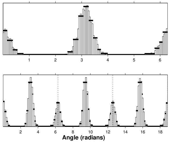

As a footnote, one application that might not be obvious is the case of gamma-ray burst light curves which are short enough that the background is accurately constant over the duration of the burst. If all of the data are rescaled to fit on a circle, then the pre- and post- burst background would automatically be subsumed into a single block (covering intervals at the beginning and end of the observation period). This procedure would be applicable to bursting light curves of any kind if and only if the background signal is constant, so that the event rates before and after the main burst are the same.
5 Conclusions and Future Work
The Bayesian Blocks algorithm finds the optimal step function model of time series data by implementing the dynamical programming algorithm of [Jackson et al. 2005]. It is guaranteed to find the representation that maximizes any block-additive fitness function, in time of order , and replaces the greedy approximate algorithm in [Scargle 1998]. Its real-time mode triggers on the first statistically significant rate change in a data stream.
This paper addresses the following issues in the use of the algorithm for a variety of data modes: gaps and exposure variations, piecewise linear and piecewise exponential models, the prior distribution for the number of blocks, multivariate data, the empty block problem (for event data), data on the circle, dispersed data, and analysis of variance (”error analysis”). The algorithm is shown to closely approach the theoretical detection limit derived in [Arias-Castro, Donoho and Huo 2003].
Work in progress includes extensions to generalized data spaces such as those of higher dimensions (cf. [Scargle 2001c]), and speeding up the algorithm.
Acknowledgements: This work was supported by Joe Bredekamp and the NASA Applied Information Systems Research Program, and the CAMCOS program through the Woodward Fund at San Jose State University. JDS is grateful for the hospitality of the Institute for Pure and Applied Mathematics at UCLA, and the Keck Institute for Space Studies at Cal Tech. We are grateful to Glen MacLachlan and Erik Petigura for helpful comments.
Appendix A Reproducible Research: MatLab Code
This paper implements the spirit of Reproducible Research, a publication protocol initiated by John Claerbout [Claerbout 1990] and developed by others at Stanford and elsewhere. The underlying idea is that the most effective way of publishing research is to include everything necessary to reproduce all of the results presented in the paper. In addition to all relevant mathematical equations and the reasoning justifying them, full implementation of this protocol requires that the data files and computer programs used to prepare all figures and tables are included. Cogent arguments for Reproducible Research, an overview of its development history, and honest assessment of its successes and failures, are eloquently described in [Donoho et al. (2008)].
Following this
discipline all of the MatLab code and data files
used in preparing this paper are available
as auxiliary material.
Included is the file ”read_me.txt” with details and
a script ”reproduce_figures.m”
that erases
all of the figure files and
regenerates them from scratch.
In some cases the default parameters
implement shorter simulation
studies than those that were used for the
figures in the paper,
but one of the features of Reproducible Research
is that such parameters and other aspects
of the code can be changed and experimented at will.
Accordingly this collection of scripts
includes illustrative exemplars of
the use of and algorithms and
serves as a tutorial for the methods.
In addition here is
a commented version of
the key fragment of the MatLab script
(named find_blocks.m)
for the basic algorithm described in this paper:
% For data modes 1 and 2:
% nn_vec is the array of cell populations.
% Preliminary computation:
block_length=tt_stop-[tt_start 0.5*(tt(2:end)+tt(1:end-1))’ tt_stop];
...
%-----------------------------------------------------------------
% Start with first data cell; add one cell at each iteration
%-----------------------------------------------------------------
best = [];
last = [];
for R = 1:num_points
   % Compute fit_vec : fitness of putative last block (end at R)
    if data_mode == 3 % Measurements, normal errors
        sum_x_1 = cumsum( cell_data( R:-1:1, 1 ) )’; %sum(x/sig^2)
        sum_x_0 = cumsum( cell_data( R:-1:1, 2 ) )’; %sum(1/sig^2)
        fit_vec=((sum_x_1(R:-1:1) ) .^ 2 ) ./( 4*sum_x_0(R:-1:1));
    else
        arg_log = block_length(1:R) - block_length(R+1);
        arg_log( find( arg_log <= 0 ) ) = Inf;
        nn_cum_vec = cumsum( nn_vec(R:-1:1) );
        nn_cum_vec = nn_cum_vec(R:-1:1);
        fit_vec = nn_cum_vec .* ( log( nn_cum_vec ) - log( arg_log ) );
    end
    [ best(R), last(R)] = max( [ 0 best ] + fit_vec - ncp_prior );
end
%-----------------------------------------------------------------
% Now find changepoints by iteratively peeling off the last block
%-----------------------------------------------------------------
index = last( num_points );
change_points = [];
while index > 1
    change_points = [ index change_points ];
    index = last( index - 1 );
end
Appendix B Mathematical Details
Partitions of arrays of data cells are crucial to the block modeling which our algorithm implements. This appendix collects a few mathematical facts about partitions and the nature of independent events.
B.1 Definition of Partitions
A partition of a set is a collection of its subsets that add up to the whole with no overlap. Formally, a partition is a set of elements, or blocks satisfying
| (43) |
and
| (44) |
Note that these conditions apply to the partitions of the time series data by sets of data cells. The data cells themselves may or may not partition the whole observation interval, as either the completeness in eq. (43) or the no-overlap condition in eq. (44) may be violated.
B.2 Reduction of Infinite Partition Space to a Finite One
For a continuous independent variable, such as time, the space of all possible partitions is infinitely large. We address this difficulty by introducing a construct in which and its partitions are represented in terms of a collection of discrete data cells in one-to-one correspondence with the measurements.66 6 The cells may form a partition of , as for example with event data with no gaps (see §3.1), but it is not necessary that they do so. The blocks which make up the partitions are sets of data cells contiguous with respect to time-order of the cells. I.e. a given block consists of exactly all cells with observation times within some sub-interval of .
Now consider two sets of partitions of : (a) all possible partitions (b) all possible collections of cells into blocks. Set (a) is infinitely large since the block boundaries consist of arbitrary real numbers in , but set (b) is a finite subset of (a). Nevertheless, under reasonable assumptions about the data mode, any partition in (a) can be obtained from some partition in (b) by deforming boundaries of its blocks without crossing a data point. Because the potential of a block to be an element of the optimum partition (see the discussion of block fitness in §3) is a function of the content of the cells, such a transformation cannot substantially change the fitness of the partition.
B.3 The Number of Possible Partitions
How many different partitions of cells are possible? Represent a partition by an ordered set of zeros and ones, with one indicating that the corresponding time is a change-point, and zero that it is not. With two choices at each time, the number of combinations is
| (45) |
Except for very short time series this number is too large for an exhaustive search, but our algorithm nevertheless finds the optimum over this space in a time that scales as only .
B.4 A Result for Subpartitions
We here define subpartitions and prove an elementary corollary that is key to the algorithm.
Definition: a subpartition of a given partition is a subset of the blocks of .
It is obvious that a subpartition is a partition of that subset of consisting of those blocks. Although not a necessary condition for the result to be true, in all cases of interest here the blocks in the subpartition are contiguous, and thus form a partition of a subinterval of . It follows that:
Theorem: A subpartition of an optimal partition is an optimal partition of the subset that it covers.
For if there were a partition of , different from and fitter than , then combining it with the blocks of P not in would, by the block additivity condition, yield a partition of fitter than P, contrary to the optimality of P.
We will make use of the following corollary:
Corollary: removing the last block of an optimal partition leaves an optimal partition.
B.5 Essential Nature of the “Poisson” Process
The term Poisson process refers to events occurring randomly in time and independently of each other. That is, the times of the events,
| (46) |
are independently drawn from a given probability distribution. Think of the events as darts thrown randomly at the interval. If the distribution is flat (i.e. the same all over the interval of interest) we have a constant rate Poisson process. In this special case a point is just as likely to occur anywhere in the interval as it is anywhere else; but this need not be so. What must be so in general – the essential nature of the Poisson process from a physical point of view – is the above-mentioned independence: each dart is not at all influenced by the others. Throwing darts that have feathers or magnets, although random, is not a Poisson process if these accoutrements cause the darts to repel or attract each other.
This key property of independence determines all of the other features of the process. Most important are a set of remarkable properties of interval distributions (see e.g. [Papoulis 1965]). The time interval between a given point and the time of the next event is exponentially distributed
| (47) |
where . The remarkable aspect is that it does not matter how is chosen; in particular the distribution is the same whether or not an event occurs at . This fact makes the implementation of event-by-event exposure straightforward (§1.8).
Note that we have not mentioned the Poisson distribution itself. The number of events in a fixed interval does obey the Poisson distribution, but this result is subsidiary to, and follows from, event independence. In this sense a better name than Poisson process is independent event process.
In representing intensities of such processes, one scheme is to represent each event as a delta-function in time. But a more convenient way to extract rate information incorporates the time intervals77 7 A method for analyzing event data based solely on inter-event time intervals has been developed in ([Prahl 1996]). between photons. Specifically, for each photon consider the interval starting half way back to the previous photon and ending half way forward to the subsequent photon. This interval, namely
| (48) |
is the set of times closer to than to any other time,88 8 These intervals form the Voronoi tessellation of the total observation interval. See ([Okabe, Boots, Sugihara and Chiu 2000]) for a full discussion of this construct, highly useful in spatial domains of 2, 3, or higher dimension; see also ([Scargle 2001a, Scargle 2001c]). and has length equal to the average of the two intervals connected by photon , namely
| (49) |
Then the reciprocal
| (50) |
is taken as an estimate of the signal amplitude corresponding to observation . When the photon rate is large, the corresponding intervals are small.

demonstrates the data cell concept, including the simple modifications to account for variable exposure and for weighting by photon energy.
[Prahl 1996] has derived a statistic for event clustering in Poisson process data that tests departures from the known interval distribution by evaluating the likelihood over a restricted interval range. Prahl’s statistic is
| (51) |
where is the interval between events and , and
| (52) |
is the empirical mean interval. In other settings, the fact that this statistic is a global measure of departure of the distribution (used here only locally, over one block) may be useful in the detection of periodic, and other global, signals in event data.
Appendix C Other Block Fitness Functions
This appendix describes fitness function for a variety of data modes.
C.1 Event Data: Alternate Derivation
The Cash statistics used to derive the fitness function in Eq. (19) is based on representation of event times as real numbers. Of course time is not measured with infinite precision, so it is interesting to note that a more realistic treatment yields the same formula.
Typically the data systems’ finest time resolution is represented as an elementary quantum of time, which will be called a tick since it is usually set by a computer clock. Measured values are expressed as integer multiples of it (cf. §2.2.1 of [Scargle 1998]). We assume that , the number of events (e.g. photons) detected in tick obeys a Poisson distribution:
| (53) |
where is the length of the tick. The event rates and are counts per second and per tick, respectively. Time here is given in units such as seconds, but a representation in terms of (dimensionless) integer multiples of is sometimes more convenient.
Due to event independence the block likelihood is the product of these individual factors over all ticks in the block. Assuming all ticks have the same length this is:
| (54) |
where is the number of ticks in block . Note that non-events are included via the factor for each tick with . When this expression is used to compute the likelihood for the whole interval (i.e. product of the block likelihoods over all blocks of the model) the denominator contributes the factor
| (55) |
where on the right-hand side the product is over all the ticks in the whole interval. For low event rates where never exceeds , this quantity is unity. No matter what it is a constant, fixed once and for all given the data; in model comparison contexts it is independent of model parameters and hence irrelevant. Dropping it, noting that is just Collecting together all factors for ticks with the same number of events eq. (54) simplifies to
| (56) |
where is the number of ticks in the block with events. Noting that
| (57) |
where is the total number of events in block , we have simply
| (58) |
In order for the model to depend on only the parameters defining the block edges, we need to eliminate from eq. (58). One way to do this is to find the maximum of this likelihood as a function of , which is easily seen to be at , yielding
| (59) |
The exponential contributes the overall constant factor to the full model. Moving this ultimately irrelevant factor to the left-hand side, noting that , and taking the log, we have for the maximum-likelihood block fitness function
| (60) |
equivalent to Eq. (19).
An alternative way to eliminate is to marginalize it as in the Bayesian formalism. That is, one specifies a prior probability distribution for the parameter and integrates the likelihood in Eq. (58) times this prior. Since the current context is generic, not devoted to a specific application, we seek a distribution that expresses no particular prior knowledge for the value of . It is well known that there are several practical and philosophical issues connected with such so-called non-informative priors. Here we adopt this simple flat, normalized prior:
| (61) |
where the normalization condition yields
| (62) |
Thus eq. (58), with marginalized, is the posterior probability
| (63) | |||||
| (64) |
where . In terms of the incomplete gamma function
| (65) |
we have, utilizing ,
| (66) |
The infinite range , gives
| (67) |
This prior is unnormalized (and therefore sometimes regarded as improper). Technically approaches zero as , but is retained here in order to formally retain the scale invariance to be discussed at the end of this section.
Another commonly used prior is the so-called conjugate Poisson distribution
| (68) |
As noted by [Gelman, Carlin, Stern, and Rubin 1995] this “prior density is, in some sense, equivalent to a total count of -1 in prior observations,” a relation that might be useful in some circumstances. The normalization constant , and with this prior the marginalized posterior probability distribution is
| (69) |
yielding
| (70) |
Note that for this prior and posterior reduce to those in Eqs. (28) and (29) of [Scargle 1998].
Equations (19), (66), (67) and (70) are all invariant under a change in the units of time. The case of eq. (67) is slightly dodgy, as mentioned above, but otherwise is a direct result of expressing and as dimensionless counts, of events and time-ticks, respectively. (Further, in the case of eq. (66), and are dimensionless.) As mentioned above, the simplicity of eq. (19) recommends it in general, but specific prior information (e.g. as represented by eq. 68) may suggest use of one of the other forms.
C.2 0-1 Event Data: Duplicate Time Tags Forbidden
In Mode 2 duplicate time tags are not allowed, the number of events detected at a given tick is or , and the corresponding tick likelihood is:
| (71) | |||||
| (72) |
where is the model event rate, in events per unit time. From the Poisson distribution is the probability of an event, and that of no event. Note that or interchangeably specify the event rate. Since independent probabilities multiply, the block likelihood is the product of the tick likelihoods:
| (73) |
where is the number of ticks in block and is the number of events in the block.
There are again two ways to proceed. The maximum of this likelihood occurs at and is
| (74) |
Using the logarithm of the maximum likelihood,
| (75) |
yields the fitness function, additive over blocks.
As in the previous sub-section, an alternative is to marginalize :
| (76) |
where is the prior probability distribution for the rate parameter. With the flat prior in eq. (61)99 9 In [Scargle 1998] we used as the independent variable, and chose a prior flat (constant) as a function of . Here, we use a prior flat as a function of the rate parameter. the posterior, marginalized over is
| (77) |
Changing variables to , with , this integral becomes
| (78) |
with , and expressible in terms of the incomplete beta function
| (79) |
as follows:
| (80) |
The case yields the ordinary beta function:
| (81) |
differing from Eq. (21) of [Scargle 1998] by one in the second argument, due to the difference between a prior flat in and one flat in . All of the equations (75), (80), and (81), can be used as fitness functions in the global optimization algorithm and, as with Mode 1, are invariant to a change in the units of time.
A brief aside: one might be tempted to use intervals between successive events instead of the actual times, since in some sense they express rate information more directly. However, as we now prove, the likelihood based on intervals is essentially equivalent to that in eq. (58). It is a classic result [Papoulis 1965] that intervals between (time-ordered) consecutive independent events (occurring with a probability uniform in time, with a constant rate ) are exponentially distributed:
| (82) |
where is the unit step function:
Pretend that the data consists of the inter-event intervals, and that one does not even know the absolute times. The likelihood of our constant-rate Poisson model for interval is
| (83) |
so the block likelihood is
| (84) |
the same as in eq. (58), except that here is the number of inter-event intervals, one less than the number of events.
[Prahl 1996] derived a statistic for event clustering, by testing for significant departures from the known interval distribution, by evaluating the likelihood over a restricted interval range. This statistic is
| (85) |
where is the interval between events and , is the number of terms in the sum, and
| (86) |
is the empirical mean of the relevant intervals. In some settings, the fact that this statistic is a global measure (as opposed to the local – over one block at a time – ones used here) may be useful in the detection of global signals, such as periodicities, in event data.
C.3 Time-to-Spill Data
As discussed in §2.2.3 of [Scargle 1998], reduction of the necessary telemetry rate is sometimes accomplished by recording only the time of detection of every Sth photon, e.g. with S=64 for the BATSE time-to-spill mode. This data mode has the attractive feature that its time resolution is greater when the source is brighter (and possibly more active, so that more time resolution is useful). With slightly revised notation the likelihood in Eq. (32) of [Scargle 1998] simplifies to
| (87) |
where is the number of spill events in the block, and is as usual the length of the block in ticks. With this is identical to the Poisson likelihood in Eq.(54), and in particular the maximum likelihood is at and the corresponding fitness function is
| (88) |
just as in Eq. (19) with , and with the same property that the unit in which block lengths are expressed is irrelevant.
C.4 Point measurements: Alternative Form
An alternative form can be derived by inserting (38) instead of (36) into the log of Eq. (30) as in §3.3. The result is:
| (89) |
Expanding the square gives
| (90) |
| (91) |
| (92) |
| (93) |
yielding
| (94) |
where
| (95) |
is the weighted average variance of the measured signal values in the block. It makes sense that the block fitness function is proportional to the negative of the variance: the best constant model for the block should have minimum variance.
C.5 Point measurements: Marginal Posterior, Flat Prior
First, consider the simplest choice, the flat, unnormalizable prior
| (96) |
giving equal weight to all values. The marginal posterior for block is then, from Eq. (30),
| (97) |
Using the definitions introduced above in eqs. (31), (32), and (33) we have
| (98) |
Using standard “completing the square,” letting , giving
| (99) |
and then using
| (100) |
we have
| (101) |
From this result, the log-posterior fitness function is
| (102) |
where
| (103) |
and the subscript refers to the fact that the marginal posterior was obtained with the unnormalized prior. The second and third terms in Eq. (102 ) are invariant under the transformation (42). Further, since the integral of with respect to must be dimensionless, we have , so and have the same -dependence, yielding a formal invariance for (102). However the prior in eq. (96) is not normalizable, so that technically is undefined. A way to make practical use of this formal invariance is simply to include a constant that has the proper dimension ().
C.6 Point Measurements: Marginal Posterior, Normalized Flat Prior
Marginalizing the likelihood in eq. (30) with the prior in eq. (61), yields for the marginal posterior for block :
| (104) |
As before
| (105) |
Now complete the square by letting , giving
| (106) |
so we have
| (107) |
where
| (108) |
Finally, introducing the error function
| (109) |
we have
| (110) |
Taking the log gives the final expression
| (111) |
where the subscript indicates the fact that this result is based on the finite-range prior in eq. (61). Note that this fitness function is manifestly invariant under the transformation in eq. (42), for the same reasons discussed at the end of the previous section, plus the invariance of . In the limits and , , and we recover eq.(102) – but remember that in this limit the invariance is only formal.
C.7 Point Measurements: Marginal Posterior, Gaussian Prior
Finally, consider using the following normalized Gaussian prior for :
| (112) |
corresponding to prior knowledge that roughly speaking most likely lies in the range , with a normal distribution. This prior is not to be confused with the Gaussian form for the likelihood in eq. (29).
Eq. (30), when is marginalized with this prior, becomes
| (113) |
so with
| (114) |
| (115) |
C.8 Data with Dispersed Measurements
Throughout it has been presumed that two things are small compared to any relevant time scales: errors in the determination of times of events, and the intervals over which individual measurements are obtained as averages. These assumptions justify treatment of the corresponding data modes as points in §3.1 and §3.3 respectively. Below are discussions of data that are dispersed because of (1) random errors in event times and (2) measurements that are summations or averages over non-negligible intervals. Binned data, an example of the latter, have already been treated in §3.2 and are not discussed here.
A simple ad hoc way to deal with both of these situations is to compute kernel functions for each data point, representing the window or error distribution in either of the two above contexts. Each such function would be centered at the corresponding measured value, evaluated at all of the data points, and normalized to represent unit intensity. Each such kernel would be maximum at the data point at which it is centered, but distribute some weight to the other data cells. The sum of all of these kernels would then be a set of weights at each measurement, which could then be treated as ordinary event data but with fractional rather than unit weights. The ad hoc aspect of this approach lies in the way the fitness function is extended. The following sub-sections provide more rigorous analysis.
C.8.1 Uncertain Event Locations
Timing of events is always uncertain at some level. Here we treat the case where the error distribution is wide enough to make the point approximation inappropriate. Rare for photon time series, with microsecond timing errors, this situation is more common in other contexts and with other independent variables. With overlapping error distributions even the order of events can be uncertain. In the context described in §1.4 one often wants to construct histograms from measurements with errors – errors that may be different for each point (then called heteroscedastic errors).
A simple modification of the fitness function described in §3.1 addresses this kind of data. On the right-hand side of Eq. (19) quantifies the contribution of the individual events within block . In extending the reasoning leading to this fitness function, the main issue concerns events with error distributions that have fractional overlap with the extent of block – for events distributed entirely outside (inside) obviously contribute in no way (fully) to block fitness. By the law for the sum of probabilities of independent events, in the log-likelihood implicit in Eqs. (17) and (18) is replaced by the sum of the areas under the probability distributions overlapping block , namely summed over all events with significant contribution to block , and is the integral of the overlapping part of the error distribution, a fraction between and . Thus we have
| (117) |
in place of Eq. (19), with the analogous constant term on the left-hand side of that equation dropped. This result holds because a given datum falling inside and outside a block are mutually exclusive events.
Implementing this relationship
in the algorithm is easily accomplished.
For a given event and the interval assigned to it
(cf. Figure 12
in §B.5)
sum the overlap fractions with that interval
of all events
– including that event itself.
These quantities could be approximated
with very simple or complex quadrature
schemes, depending on the context and
the way in which the relevant distributions
are represented.
Normally the array nn_vec, as in the
code fragment in §A, is all 1’s
(or counts of events with identical time-tags there are any);
but here replace it with these summed event weights.
This construction automatically assigns the
correct fractional weights to the block with
no further alteration of the algorithm.
C.8.2 Measurements in Extended Windows
This section discusses the case of distributed measurements in the sense that the time of measurement is either uncertain or is effectively an interval rather than a point. (This is different from the use of this term in §3.3 to describe the distribution of the measurement error in the dependent variable.) Measurements may refer to a quantity averaged over a range of values of , not at a single time as in §§3.3, C.4, C.5, C.6, and C.7. In the context of histograms (§1.4) the measured quantity becomes the independent variable, and the dependent variable is an indicator marking the presence of the measurement there. In both cases the measurement can be thought of as distributed over an interval, not just at a point.
In this case the data cell array would be augmented by the inclusion of a window function, indicating the variation of the instrumental sensitivity:
| (118) |
where describes, for the value reported as , the relative weights assigned to times near .
This is a nontrivial complication if the window functions overlap, but can nevertheless be handled with the same technique.
We assume the standard piece-wise constant model of the underlying signal, that is, a set of contiguous blocks:
| (119) |
where each block is represented as a boxcar function:
the are the change-points, satisfying
| (123) |
and the are the heights of the blocks.
The value of the observed quantity, , at , under this model is
so we can write
| (129) |
where
| (130) |
is the inner product of the -th weight function with the support of the -th block. The analysis in [Bretthorst 1988] shows how do deal with the non-orthogonality that is generally the case here.1010 10 If the weighting functions are delta functions, it is easy to see that is non-zero if and only if lies in block , and since the blocks do not overlap the product is zero for , yielding orthogonality, . And of course there can be some orthogonal blocks, for which there happens to be no “spill over”, but these are exceptions.
The averaging process in this data model induces dependence among the blocks. The likelihood, written as a product of likelihoods of the assumed independent data samples, is
| (131) | |||||
| (132) | |||||
| (133) | |||||
| (134) |
where
| (135) |
After more algebra and adopting a new notation, symbolized by
| (136) |
and
| (137) |
we arrive at
| (138) |
where
| (139) |
The last two equations are equivalent to Eqs. (3.2) and (3.3) of [Bretthorst 1988], so that the orthogonalization of the basis functions and the final expressions follow exactly as in that reference.
C.9 Piecewise Linear Model: Event Data
Here we outline the computations of a fitness function for the piecewise linear model in the case of event data. This means that the event rate for a block is assumed to be linear, as in Eq. (1).
For convenience we take the fiducial time to be , the time at the end of the block. Take to be the time at the beginning, so is the length of the block, and the signal is at the beginning of the block and at the end, and varies linearly in between.
The block likelihood for the case of event data is
| (140) |
where the sum is over the events in the block and the integral is over the time interval covered by the block. Simplifying we have
| (141) |
| (142) |
Now let’s compute the maximum likelihood as a function of and , starting by setting
| (143) |
so that at the maximum of this likelihood we have
| (144) |
and therefore
| (145) |
| (146) |
| (147) |
| (148) |
| (149) |
| (150) |
| (151) |
| (152) |
| (153) |
| (154) |
| (155) |
C.10 Piecewise Exponential Model: Event Data
In this case we model the signal as varying exponentially across the time interval contained in the block. Denoting the times beginning and ending the block as and , and taking the latter as the fiducial time in Equation (2), the signal is at the beginning of the block and at the end.
Much as in §C.9 the block likelihood for the case of event data is the follow expression involving a sum over the events in the block and an integral over the time interval covered by the block:
| (156) |
| (157) |
where is the length of the block.
Now let’s compute the maximum likelihood as a function of and :
| (158) |
and therefore at the maximum we have
| (159) |
| (160) |
| (161) |
| (162) |
| (163) |
where
| (164) |
| (165) |
To solve for the value of that makes this derivative zero (to find the maximum of the likelihood) we will use Newton’s method to find the zeros of
| (166) |
where
| (167) |
is the mean of the differences between the event times and the time at the end of the block. The iterative equation is
| (168) |
and since is a constant we have
| (169) |
| (170) |
and defining
| (171) |
we have
| (172) |
and
| (173) |
References
- [Arias-Castro, Donoho and Huo 2003] Arias-Castro, E., , Donoho, D., and Huo, X. 2003, “Near-Optimal Detection of Geometric Objects by Fast Multiscale Methods,” preprint.
- [Band 2002] Band, D. (2002), “A Gamma-Ray Burst Trigger Toolkit,” Astrophys.J., 578, 806-811 (arxiv.org/abs/astro-ph/0205548)
- [Bellman 1961] Bellman, R. (1961), “On the approximation of curves by line segments using dynamic programming, Communications of the ACM, Vol. 4 No. 6, p.284.
- [Bretthorst 1988]
Bretthorst, G. Larry (1988),
Bayesian Spectrum Analysis and Parameter
Estimation, Lecture Notes in Statistics,
Springer-Verlag.
http://bayes.wustl.edu/ - [Capra 2007] Fritjof Capra (2007) The Science of Leonardo, Doubleday: New York
- [Cash 1979] Cash, W., Parameter-Estimation in Astronomy through Application of the Likelihood Ratio, Astrophysical Journal, 228, 939Ð947
- [Claerbout 1990] Claerbout, J. (1990) Active documents and reproducible results, Stanford Exploration Project Report 67, 139-144
- [Coram 2002]
Coram, Marc, (2002), personal communication and Ph. D.
thesis, Nonparametric Bayesian Classification,
www-stat.stanford.edu/~mcoram/ - [Donoho 1994] Donoho, D., (1994), Smooth Wavelet Decompositions with Blocky Coefficient Kernels, in Recent Advances in Wavelet Analysis, L Schumaker and G. Webb, eds., Academic Press, pp. 259-308.
- [Donoho and Johnstone 1998] Donoho, D., and Johnstone, I. (1998), Minimax estimation via wavelet shrinkage. Ann. Statist., 26, 879-921.
- [Donoho et al. (2008)]
Donoho, D., Maleki, A., Rahman, I.,
Shahram, M., and Stodden, V. (2009),
15 Years of Reproducible Research in
Computational Harmonic Analysis.
Computing in Science and Engineering, 11, 8-18.
http://stats.stanford.edu/~donoho/Reports/2008/15YrsReproResch-20080426.pdf - [Dreyfus 2002] Dreyfus, S. (2002). “Richard Bellman on the Birth of Dynamic Programming,” Operations Research, 50, 48Ð51.
- [Efron and Tibshirani 1998] Efron, B. and Tibshirani, R. (1998) An Introduction to the Bootstrap, CRC Press LLC: New York
- [Fenimore et al. 2001] Fenimore, E., Palmer, D., Galassi, M., Tavenner, T., Barthelmy, S., Gehrels, N., Parsons, A., Tueller, J. (2001), “The Trigger Algorithm for the Burst Alert Telescope on Swift,” in Gamma-Ray Burst and Afterglow Astronomy 2001, Ricker and Vanderspek (eds), AIP, 662, 491, astro-ph/0408514
- [Gelman, Carlin, Stern, and Rubin 1995] Gelman, A., Carlin, J., Stern, H., and Rubin, D., Bayesian Data Analysis, Chapman & Hall, London: 1995.
- [Hogg 2008]
Hogg, D. W. (2008),
“Data analysis recipes: Choosing the binning for a histogram,”
http://arxiv.org/abs/0807.4820
- [Hubert, Arabie, and Meulman 2001] Hubert, L., Arabie, P., and Meulman, J., 2001, Combinatorial Data Analysis: Optimization by Dynamic Programming, SIAM: Philadelphia
- [Jackson et al. 2005] “An algorithm for optimal partitioning of data on an interval,” Jackson, B., Scargle, J.D., Barnes, D., Arabhi, S., Alt, A., Gioumousis, P., Gwin, E., Sangtrakulcharoen, P., Tan, L., and Tun Tao Tsai, IEEE Signal Processing Letters Vol.12, No. 2, 105- 108
- [Lin, Keogh, Lonardi and Chiu 2003]
A symbolic representation of time series, with implications for streaming algorithms, DMKD ’03 Proceedings of the 8th ACM SIGMOD workshop on Research issues in data mining and knowledge discovery. Also
www.cs.ucr.edu/~eamonn/SAX.htm. - [McLean et al. 2003] McLean, K., Fenimore, E., Palmer, D., Barthelmy, S., Gehrels, N., Krimm, H., Markwardt, C., and Parsons, A. (2003), “Setting the Triggering Threshold on Swift, in proceedings of the Gamma-Ray Bursts: 30 Years of Discovery conferance in Sante Fe NM, Fenimore and Galassi (eds), AIP, astro-ph/0408512
- [Norris Gehrels and Scargle 2010] Norris, J., Gehrels, N., and Scargle (2010) Ap. J., 717, 411
- [Norris Gehrels and Scargle 2011] Norris, J., Gehrels, N., and Scargle (2011) Ap. J., 735, 23
- [Okabe, Boots, Sugihara and Chiu 2000] Okabe, A., Boots, B., Sugihara, K., and Chiu, S. N. (2000), Spatial Tessellations: Concepts and Applications of Voronoi Diagrams, John Wiley and Sons, Ltd., New York, Second Edition
- [Ò Ruanaidh and Fitzgerald 1996] Ò Ruanaidh, J. J. & Fitzgerald, W. J., 1996, Numerical Bayesian Methods Applied to Signal Processing, Springer: New York.
- [Papoulis 1965] Papoulis, A, 1965, Probability, Random Variables, and Stochastic Processes, McGraw-Hill: New York.
- [Prahl 1996] Prahl, J., “A fast unbinned test on event clustering in Poisson processes,” astro-ph/9909399.
- [Qin et al. 2012] Qin, Y., Liang, E-W., Yi, S-X., Liang, Y-F., Lin, L., Zhang, B-B., Zhang, J., Lu, H-J., Lu, R-J., Lu, L-Z. and Zhang, B. (2012) “Duration Distribution of Fermi/GBM Gamma-Ray Bursts: Instrumental Selection Effect of the Bimodal T90 Distribution,” submitted to Ap. J.
- [Scargle 1998] Scargle, J., 1998, “Studies in Astronomical Time Series Analysis. V. Bayesian Blocks, A New Method to Analyze Structure in Photon Counting Data”, Astrophysical Journal, 504, p. 405-418, Paper V.
- [Scargle 2001a] Scargle, J. D., (2001), Bayesian Blocks: Divide and Conquer, MCMC, and Cell Coalescence Approaches, in Bayesian Inference and Maximum Entropy Methods in Science and Engineering, 19th International Workshop, Boise, Idaho, 2-5 August, 1999. Eds. Josh Rychert, Gary Erickson and Ray Smith, AIP Conference Proceedings, Vol. 567, p. 245-256.
- [Scargle 2001c] Scargle, J. D., (2001), “Bayesian Blocks in Two or More Dimensions: Image Segmentation and Cluster Analysis,” Contribution to Workshop on Bayesian Inference and Maximum Entropy Methods in Science and Engineering (MAXENT 2001), Johns Hopkins University, Baltimore, MD USA on August 4-9, 2001.
- [Schmidt 1999] Schmidt, M. (1999), “Derivation of a Sample of Gamma-Ray Bursts from BATSE DISCLA Data,” in Proc. of the 5th Huntsville Gamma Ray Burst Symposium, Oct. 1999, ed. R.M. Kippen, AIP astro-ph/0001122
- [Tompkins 1999]
Tompkins, W. (1999),
Applications of Likelihood Analysis
in Gamma-Ray Astronomy,
Stanford Ph. D. Thesis,
http://arxiv.org/pdf/astro-ph/0202141v1.pdf - [Tong 1990] Tong, H. (1990). Non-Linear Time Series: A Dynamical System Approach. Oxford University Press.
- [Way Gazis and Scargle 2011] Way, M., Gazis, P. and Scargle, J., Structure in the 3D Galaxy Distribution: I. Methods and Example Results, Ap. J., 727