On proton synchrotron blazar models: the case of quasar 3C 279

By combining equation (7) with the integrated power over all synchrotron frequencies (equation 8) one obtains the total comoving synchrotron power

that is related to the total observed $\gamma$-ray luminosity $L_{\gamma}^{\rm obs}\approx 10^{48}$ ers/s by the usual relation $L_{\gamma}^{\rm obs}=\delta^{4}L$. This leads to our second relation

where $C_{2}^{\prime}=2C_{2}V(\nu_{\gamma}^{\rm obs})^{1/2}/\ln(\gamma_{\rm max})m_{\rm p}c^{2}$. For a specific magnetic field we find a relation of proportionality

which is also verified by the detailed numerical treatment (see section 3.2). We note that the proportionality at the right hand side of relation (13) holds only if the magnetic field is not strong enough to cause significant proton cooling due to synchrotron radiation.

The maximum proton Lorentz factor has remained so far undetermined. However, the fact that the proton gyroradius $r_{\rm g}$ should be less or equal than the size of the blob $R$ (Hillas, 1984) sets a strong upper limit

where $\kappa$ is a scaling factor that takes values less or equal to unity. It has been introduced in order to take into account the fact, that good fits can be obtained for certain parameter sets with $\gamma_{\rm max}<<eBR/m_{\rm p}c^{2}$; as an example see the parameters used for figure 4. By combining the above relation with equation (7) we find a lower limit for the Doppler factor

where

Automatic quenching of $\gamma$-rays was irrelevant to the derivation of the relations presented up to this point. Actually, it will not play any role in the evolution of the system if the magnetic field is weak enough. There is, in other words, a necessary but not sufficient condition for the operation of automatic quenching, the so-called feedback criterion. This can be derived from the requirement that the magnetic field is strong enough so that the synchotron photons of the automatically produced pairs lie above the threshold for further photon-photon absorption on the $\gamma$-rays (Stawarz & Kirk, 2007; Petropoulou & Mastichiadis, 2011; Petropoulou & Mastichiadis, 2012). This requirement sets a lower limit for the magnetic field

where $B_{\mathrm{c}r}=4.4\times 10^{13}$ G. If we set $\epsilon_{\gamma}=\epsilon_{\gamma}^{\rm obs}(z+1)\delta^{-1}$ and use equations (7) and (14) we find an expression for the magnetic field $B_{\mathrm{q}}$, below which the feedback criterion is not satisfied. This involves only physical constants except for the size of the blob $R$ and the scaling factor $\kappa$:

In order to have an estimate, the above expression gives $B_{\mathrm{q}}\approx 3.5$ G for $R=3\times 10^{16}$ cm and $\kappa=1$. Note that for a given $R$ this is also the minimum value of $B_{\mathrm{q}}$. One could also express $B_{\mathrm{q}}$ in terms of $\gamma_{\rm max}$ as

as long as $\gamma_{\rm max}$ does not exceed the value given by equation (14) for $\kappa=1$. From equation (12) becomes evident that if the Doppler factor decreases then the proton energy density or the proton compactness equivalently should increase in order to obtain the same observed luminosity. If, however, the feedback criterion is satisfied, then the proton compactness is bounded from above. This immediately sets a lower limit for the Doppler factor. We proceed next to obtain an expression of $\delta_{\rm min}$. In previous work we have obtained an analytical expression for the critical $\gamma$-ray compactness (see equation (34) of Petropoulou & Mastichiadis (2011)), which will prove very useful for our analytical calculations

where $C_{4}=\left(2\epsilon_{\gamma}^{\rm obs}/\sigma_{0}^{2}B_{\mathrm{c}r}m_{\rm e}c^{2}\right)^{1/2}$ and $\sigma_{0}=4/3$ is a normalization constant. The $\gamma$-ray compactness is defined as $\ell_{\gamma}=L\sigma_{\mathrm{T}}/4\pi Rm_{\rm e}c^{3}$. Using equation (11) expressed in terms of proton compactness $\ell_{\rm p}$ instead of total proton number $N_{\rm p}$ we can rewrite the above definition as

where

In order to avoid an overproduction of soft photons that would violate the upper limit set by the X-ray observations we require that $\ell_{\gamma}\leq\lambda\ell_{\rm cr}^{\rm inj}$, where $\lambda$ is a numerical factor between 1 and 10; the exact value can be estimated only numerically. This requirement defines a maximum proton compactness

which, if inserted in equation (12), gives the minimum Doppler factor

We note that $\delta_{\rm min}$ given by the equation above is a rather robust limit, since it depends weakly on the physical quantities. We note also that the numerical factor $\lambda$ appears in the above expression raised to the power $-2/7$ and therefore it does not affect the value of $\delta_{\rm min}$ severely.

Summarizing, we have found that for $B<B_{\mathrm{q}}$, the minimum value of the Doppler factor is defined by the requirement that the gyroradius is less than the blob size and it has a very strong dependence on the magnetic field, i.e. $\delta_{\rm min}\propto B^{-3}$. On the other hand, for $B\geq B_{\mathrm{q}}$ , it is defined by the requirement that the proton compactness cannot exceed a critical value. The dependence on the magnetic field is in this case weak, i.e. $\delta_{\rm min}\propto B^{-1/7}$.

Estimations of the equipartition magnetic field of a relativistically moving blob are common in the literature and are based on fitting the low-frequency synchrotron spectrum of a power-law distribution electrons to radio observations (Pacholczyk, 1970). Here we derive an expression for the equipartition magnetic field in a proton-synchrotron blazar model, replacing the power-law distribution of electrons with protons and the radio with VHE $\gamma$-ray observations. From equation (12) we find that the comoving proton energy density is given by

where $A=L_{\gamma}^{\rm obs}{C_{2}^{\prime}}^{-1}$. Assuming that the energy density of secondary leptons is negligible with respect to that of protons, we can compute the equipartition field $B_{\rm eq}$

or

We note that here and in what follows the convention $Q_{X}\equiv Q/10^{X}$ in cgs units was adopted unless stated otherwise. The above expression apart from the numerical constant, is identical to that found using equipartition arguments in the context of a leptonic model (see e.g. equation (A7) of Harris & Krawczynski (2002)). In the previous subsection it was found that the Doppler factor of the blob has a minimum value $\delta_{\rm min}$ and its functional dependence on $B$ was also derived. One can therefore investigate whether or not the system can achieve equipartition under the requirement that $\delta=\delta_{\rm min}$ and in this case estimate $B_{\rm eq}$ using equation (27).

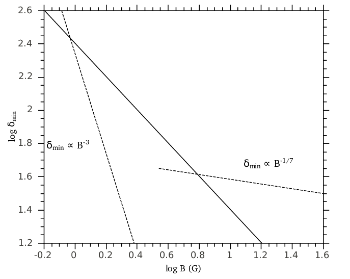
Figure  1 shows $\delta_{\rm min}(B)$ given by equations (15) and (24) and the line $\delta\propto B_{\rm eq}$ for $R=3\times 10^{16}$ cm and $\lambda=5$. The discontinuity occurs at $B_{\mathrm{q}}$, where the functional dependence of $\delta_{\rm min}$ on $B$ changes. The expressions derived should not be trusted in the neighbourhood of $B_{\mathrm{q}}$. The points of intersection correspond to the equipartition magnetic field values. The physical system can be found in equipartition either moving with a high Doppler factor and being weakly magnetized or moving with a modest Doppler factor and containing a stronger magnetic field.

A robust result of our treatment, which also differentiates it from other works, is that for a given magnetic field there is a minimum value for the Doppler factor of the flow that is set either by the gyroradius or by automatic quenching arguments. Whenever the analysis of a physical problem leads in the derivation of an extremum for some parameter, it is interesting to study the properties of the physical system in this case. For this reason, in the following we present how the particle energy density and the power of the jet depend on the magnetic field in the particular case of $\delta=\delta_{\rm min}$. Using equations (15), (24) and (25) we find that

and

Note the large change in the dependence of the proton energy density on $B$. The last proportionality is not valid for very high values of the magnetic field, since in this case the synchrotron cooling becomes important and is against our initial assumptions.

In an one-zone homogeneous model the emitting plasma is confined in a blob with radius $R$ moving with a velocity $\beta c$ and bulk Lorentz factor $\Gamma$ at an angle $\theta$ with respect to the line of sight. The radiation is further assumed to originate from a region in the jet of volume $V\approx\pi R^{3}$. The energy densities of particles, magnetic field and radiation are contributing to the jet power. Using the approximations $\theta\approx 1/\Gamma$, $\delta\approx\Gamma$ and $\beta\approx 1$ the observed jet power is given by

where $u_{\rm part}\approx u_{\rm p}$, $\beta=\sqrt{1-1/\Gamma^{2}}$ and $u_{\rm rad}$ is the radiation energy density, which for simplifying reasons will not be included in the following analytical calculations. It will be however taken into account in our numerical treatment of section 3. Note also that in our analytical formulation we have not included any population of ‘cold’ protons and electrons, which are physically implied by charge conservation arguments. However, their contributions to the total jet power are minor (see for example Protheroe & Mücke 2001) and would not affect our results significantly.

Inserting the expression for $u_{\rm p}$ given by equation (25) in the above relation we find that the jet power is a function only of the product $\delta\cdot B$

The jet power is minimized when the following condition holds

Comparison of equations (26) and (32) shows that whenever the system achieves equipartition the jet power also minimizes at the value

Thus, even the minimum jet power obtained in the framework of the proton-synchrotron blazar model is high compared to values inferred from pure leptonic modelling of blazar emission; see e.g. Celotti & Ghisellini (2008). Since for a large range of $B$ values the system lies far from equipartition (see figure 1), equations (27) and (32) imply that the calculated jet power differs significantly from its minimum value.

The fact that the Doppler factor has a lower limit implies that for magnetic fields higher than a certain value $B_{\rm h}$, equation (32) cannot be further satisfied and there is no set of parameters that lead to minimization of the jet power. The characteristic value $B_{\rm h}$ can be derived by combining equations (24) and (32). It is given by:

The same holds also for weak enough magnetic fields. Thus, by combination of equations (15) and (32) one derives a second characteristic value $B_{\rm l}$ for the magnetic field, below which there is no set of parameters that could minimize the power of the jet

Therefore, the discussion above reveals another important physical aspect of $\delta_{\rm min}$; it limits the range of $B$-values among which one should choose in order to obtain the minimum power of the jet. If $\delta=\delta_{\rm min}$ the dependence of $P_{\rm jet}^{\rm obs}$ on $B$ can also be derived by combining equations (15), (24) and (31)

and

where $a_{1,2}$ and $b_{1,2}$ are constants. Note that the functional form of $P_{\rm jet}^{\rm obs}$ is not trivial and it consists of four power-law segments. We will return to this point in the next section, where we perform the numerical approach in fitting the $\gamma$- ray observations of 3C 279.

Our aim is to produce a parameter space which gives ‘good’ fits to February 2006 observations of 3C 279. Application of existing theoretical models to AGN observations leads to one set of parameters that minimizes the $\chi^{2}$-value. However, the goodness-of-fit may pose some interesting questions, especially when two very different sets of parameters may have very similar values of $\chi^{2}$. For this reason, in what follows, we do not restrict ourselves to the best fit with the minimum $\chi^{2}$-value, but we rather relax the definition of a ‘good’ fit. Thus, fits to the TeV data that have $\chi^{2}_{\rm red}<1.5$ are characterized as ‘good’ and they are obtained for different combinations of the parameters. This, as we will show in the next section, results in the formation of a parameter space instead of a single set of accepted parameter values.

Since we keep $\gamma_{\rm min}$, $s$ and $R$ fixed the number of free parameters in the context of a pure hadronic model reduces to four: $B$, $\gamma_{\rm max}$, $\ell_{\rm p}$ and $\delta$. Thus, we search for combinations of the aforementioned parameters that provide good fits to the TeV data. At the same time we have treated the X-ray observations as upper limits: As long as the proton induced emission is below the X-ray data, we assume that one can always find a fit to them by using a suitably parametrized leptonic component. On the other hand, if the emission due to photon quenching is above the X-rays, then we discard the fit. The steps of the algorithm followed are

1. 1.

   Choose a value for the magnetic field strength $B$.

2. 2.

   Choose a value for the maximum proton Lorentz factor $\gamma_{\rm max}$ starting from the highest possible value, which is imposed by the Hillas criterion (see equation (14)).

3. 3.

   Choose an injection compactness for the proton distibution $\ell_{\rm p}$. For high enough values, automatic quenching sets in and creates a soft-photon component that exceeds the X-ray observations.

4. 4.

   Choose a value for the Doppler factor $\delta$ after taking into account that the variability timescale of 3C 279 does not exceed that of one day.

For each triad $(B,\gamma_{\rm max},\ell_{\rm p})$ two values of $\delta$ can be found that correspond to fits with $\chi^{2}_{\rm red}\leq 1.5$. This can be easily explained by the parabolic shape of the $\chi^{2}_{\rm red}$ curves. Figure 2 shows $\chi^{2}_{\rm red}$ as a function of $\delta$ for $B=40$ G and $\gamma_{\rm max}=4\times 10^{9}$. Different curves correspond to different values of $\ell_{\rm p}$. The part of the curve that lies below the horizontal line with $\chi^{2}_{\rm red}=1.5$ provides good fits. Its projection on the horizontal axis defines an interval of $\delta$-values. For simplifying reasons, we consider that each monotonic branch of the $\chi^{2}_{\rm red}$-curve that lies below the horizontal line is represented only by one $\delta$-value, i.e. only by one point on the horizontal axis. Thus, for each $\ell_{\rm p}$ we find two representative values of the Doppler factor. The error we make in this case is not large since the curves are very steep. Note also that Doppler factors lying between the two representative $\delta$-values also provide good fits. If we repeat the above proceedure for various $\gamma_{\rm max}$ we can then create a parameter space for $\ell_{\rm p}$ and $\delta$ for a specific value of the $B$-field. An example is shown in figure 3 for $B=40$ G and different $\gamma_{\rm max}$. For the case considered here, $\gamma_{\rm max}$ ranges from $10^{9.6}$ (horizontally dashed area) to $10^{10}$ (vertically dashed area) with a step of 0.2 in logarithmic units. The envelope of each striped area is the result of the two representative values of $\delta$ defined for each $\ell_{\rm p}$, as previously described. Note that in a log-log plot the lines of the envelope are power laws with an exponent $-0.22$, i.e. $\delta\propto\ell_{\rm p}^{-0.22}$. This almost coincides with the value $-2/7$ found in our analytical approach (see equation 13). Values of $\gamma_{\rm max}$ outside this range do not provide good fits and are therefore discarded. Thus, the shaded areas in Figure 3 depict all the possible combinations of $\ell_{\rm p}$, $\gamma_{\rm max}$ and $\delta$ that provide good fits to the TeV observations. We note that one can use low values of the proton injection compactness $\ell_{\rm p}$ and get acceptable TeV fits but this can be done only if he/she allows the Doppler factor to take high values – this is due to the fact that the observed and blob frame luminosities are related by $L_{\rm obs}\propto\delta^{4}L_{\rm int}$, while $L_{\rm int}\propto L_{\rm p}\propto\ell_{\rm p}$. On the other hand, higher values of $\ell_{\rm p}$ naturally result in lower $\delta$ values. However, as stated earlier, we find that $\gamma-$ray quenching plays an important role when $\ell_{\rm p}$ takes higher values. In this case the spontaneously produced soft photons increase and eventually will start violating the X-ray observations, destroying the goodness of the fit. Therefore, an upper limit is imposed on the allowed values of $\ell_{\rm p}$ which implies in turn, the existence of a minimum value of the Doppler factor (see equations (23) and (24)).

Figure 4 exemplifies the effect of $\gamma$-ray absorption on the adopted values of $\ell_{\rm p}$ and $\delta$ for fitting the TeV data. The MAGIC TeV data points show the measured flux corrected for intergalactic $\gamma\gamma$ absorption. The lowest possible level of extragalactic background light (EBL) according to Primack et al. (2005) has been used for the de-absorption of the VHE $\gamma$-rays. The full line curve depicts the last good-fit spectrum we obtain for a high $\ell_{\rm p}$. Here $\ell_{\rm p}=4\times 10^{-5}$, $\gamma_{\rm max}=10^{9.8}$ and $\delta_{\rm min}=18.6$. Other parameters used for this plot are: $\gamma_{\rm min}=1$, $R=3\times 10^{16}$ cm, $B=40$ G and $s=2$. Note first that the minimum Doppler factor derived here does not violate the inequality (38) for $t_{\rm days}=1$, and second that $B^{2}\gamma_{\rm max}$ satisfies the constraint given by relation (6). The non-linear cascade due to quenching has produced a soft component that is almost at the observed X-ray flux. Any attempt to increase $\ell_{\rm p}$ further will produce a higher flux of soft photons which would violate the X-rays. To demonstrate this point further, we have ran the code for a high value of $\ell_{\rm p}=10^{-3}$. This value is well inside the quenching regime and thus should be excluded due to strong X-ray production. However, by turning artificially $\gamma\gamma$ absorption off, we inhibit the growth of the non-linear cascade and therefore a good fit can be obtained with a $\delta$ as low as 10 (dashed line). Moreover, if $\gamma\gamma$ absorption is treated in an approximate semi-analytic manner as a linear absorption process, automatic quenching of $\gamma$-rays will not even occur , since it is a purely non-linear absorption process. Therefore, no limiting value of the proton and $\gamma$-ray compactness would be found and the transition of the hadronic system to supercriticality would not be seen. As a result one would find erroneously a more extended parameter space that fits the data. In such case, the Doppler factor would not be limited to a lower value apart from the one found by the usual gyroradius arguments made in section 2.

As a next step we have obtained $\delta_{\rm min}$ for various values of the magnetic field $B$. This is depicted in figure 5, where the two branches derived analytically in the previous section (see figure 1) are clearly seen. The power law dependence of $\delta_{\rm min}$ on $B$ can be modelled as of $\delta_{\rm min}\propto B^{-\alpha}$ with $\alpha\simeq 2.85$ for the low-B branch and $\alpha\simeq 0.05$ for the high-B branch. We note that the numerically derived power-law exponents of the two branches are very close to those given by equations (15) and (24) respectively. A new feature of figure 5 is that for very strong magnetic fields, where synchrotron cooling affects a significant part of the proton power-law distribution, the minimum Doppler factor required for a good fit slightly increases with increasing $B$.

The previous analysis makes evident that acceptable fits to the TeV observations of 3C 279, within the context of the hadronic model, can be found for a large choice of magnetic fields, maximum proton energies and injection luminosities. We note also that these values are similar to the ones found in standard hadronic modelling of TeV sources (Böttcher et al., 2009).

Having already derived $\delta_{\rm min}$ for each magnetic field strength, we numerically then derive the steady state proton energy density $u_{\rm p}^{\star}\equiv u_{\rm p}(\delta_{\rm min}(B))$ and plot this quantity as a function of $B$ – see figure 6. The system becomes magnetically dominated either for high enough ($B>10$ G) or low enough ($B<0.7$ G) magnetic fields. These values should be compared to $B_{\rm h}$ and $B_{\rm l}$ given by equations (34) and (35) respectively. The two curves intersect at two points, exactly as was analytically derived (see section 2.2). At these points the two energy densities are equal and this corresponds to a minimum of the total energy density, i.e. to an equipartition between the particles and the magnetic field – we emphasize that the quantity $u_{\rm p}^{\star}$ is not the minimum particle energy density. The fact that $\delta_{\rm min}$ has a strong dependence on $B$ at low values is also reflected to $u_{\rm p}^{\star}$. Our analytical result given by equation (28) should be compared to the numerical one, i.e. $u_{\rm p}^{\star}\propto B^{8.7}$. For $B>2$ G (c.f. $B_{\rm q}$ of equation 27) the particle energy density decreases with increasing magnetic field as $B^{-1.4}$. This trend was also found analytically. The power-law exponent however is slightly different – see equation (29).

From equation (30) and for $\delta=\delta_{\rm min}(B)$ and $\ell_{\rm p}=\ell_{\rm p}(\delta_{\rm min})$ we have calculated numerically the observed jet power, which becomes a function only of the magnetic field, i.e. $P_{\rm jet}^{\rm obs}(\delta_{\rm min}(B))$. This is shown in figure 7. The function $P_{\rm jet}^{\rm obs}(\delta_{\rm min}(B))$ shows two local minima for two values of the magnetic field that differ more than one order of magnitude. For a wide range of $B$ values the calculated jet power is rather high $\approx 10^{48}-10^{49}$ erg/s in comparison to leptonic models (Celotti & Ghisellini, 2008). In a log-log plot the curve consists of four distinct power-law segments labeled with the numbers 1 to 4. In Table 1 the power-law exponents of the four segments and the corresponding analytically derived values given by equations (36) and (37) are listed. Apart from the first segment both results are in good agreement.

We have already shown that the jet power minimizes whenever $\delta$ and $B$ satisfy equation (32). In this case the system is close to a state of equipartition. We proceed to investigate whether these results are verified numerically. For each value of $B$, we therefore search among the triads $(\gamma_{\rm max},\ell_{\rm p},\delta)$ found during the fitting process for that specific set of values that minimizes the jet power. Figures 8 and 9 show respectively the minimum calculated jet power $P_{\rm jet,min}^{\rm obs}$ and the corresponding proton energy density as a function of $B$. Dashed lines are same as in figures 6 and 7 and are shown for comparison reasons.

Figure 8 shows that for $0.7\leq B\leq 10$ G all points lie close to the minimum value $P_{\rm jet,min}^{\rm obs}\simeq 6.5\times 10^{47}$ erg/s, whereas for $B>10$ G and $B<0.7$ G the minimum jet power found from our numerical data sets coincides with that calculated for $\delta=\delta_{\rm min}$ (open circles lying on the dashed line). As already discussed in section 2.3 the jet power calculated in this case is not the lowest possible minimum value, since this would be obtained for Doppler factors less than $\delta_{\rm min}$. Note that the transitions occur at $B\approx B_{\rm l}\approx 0.7\ \textrm{G}$ and $B\approx B_{\rm h}\approx 10\ \textrm{G}$.

In figure 9 one can see that $u_{\rm p}\approx u_{\rm B}$ for $B_{\rm l}\leq B\leq B_{\rm h}$, which is in complete agreement with the analytical estimates of section 2.3 . The fact that the calculated jet power is not the minimum possible one, can also be verified by the fact that the system for $B>10$ G and $B<0.7$ G is far from an equipartition state.

Each of the points shown as open circles in figures 8 and 9 corresponds to a set of parameters $(B,\gamma_{\rm max},\ell_{\rm p},\delta)$ with $\delta\geq\delta_{\rm min}$, for which the jet power is actually the minimum possible in the context of a hadronic model. In figure 10 we plot the ratio $\delta/\delta_{\rm min}$ against the magnetic field strength. For the range $0.7<B\leq 10$ G where the system is close to equipartition and the power of the jet is minimum, the ratio becomes larger than unity.

The conclusions drawn from the figures of the present section can be summarized as follows: if one chooses to model the VHE $\gamma$-ray spectra using values of $(B,\gamma_{\rm max},\ell_{\rm p},\delta)$ that minimize both the required jet power and the total energy density of the system, i.e. model the system using optimum energetic conditions, then one will be confronted with the requirement of a high Doppler factor. On the other hand, acceptable fits of the TeV data using the minimum possible Doppler factor lead to a particle dominated system and to high values of $P_{\rm jet}^{\rm obs}$ for a wide range of $B$ values, i.e. the energetic requirements in this case are higher.

Throughout the present work we have assumed that the proton distribution is a power law of exponent $s=2$. In this case the energy per logarithmic interval is the same. A different adopted value would affect the proton energy density quantitavely and therefore our energetics estimates. Let us for example consider a steep power law distribution with $s>2$. In this case more energy is injected to the protons with the minimum Lorentz factor, whereas protons at the upper cutoff of the distribution, which are responsible for the emitted radiation, carry only a small fraction of the energy. Thus, for the same proton injection compactness the total number $N_{\rm p}$ and consequently the energy density of protons $u_{\rm p}$ increases with increasing $s$. In addition, the calculated $\gamma$-ray compactness for the same $\ell_{\rm p}$ is lower. Thus, a larger proton compactness $\ell_{\rm p}$ and therefore energy density would be required in order to fit the TeV observations with the same Doppler factor. As an extreme example, we considered a very steep proton distribution with the highest value for the power law exponent predicted by acceleration theory, i.e. $s=2.5$. The fit to the TeV observations was obtained using: $B=40$ G, $\delta\approx 25$ and $\ell_{\rm p}=10^{-1.3}$. The proton energy density in this case is $u_{\rm p}=10^{4}$ erg/cm^-3, which is much higher than the values presented in section 3.3. Therefore, the case of a flat proton distribution is rather conservative as far as the energetics is concerned.

The fact that there is a very good agreement between the numerical results and our analytical expressions, where the dependence on $R$ is explicit, makes possible the prediction of the effects of a different adopted value on our results. Let us assume a more compact source with $R=3\times 10^{15}$ cm. The quantities that are directly affected by a change in the source size are listed below in descending order in terms of their dependence on $R$:

1. 1.

   The minimum Doppler factor for $B<B_{\mathrm{q}}$ (see equation 15), which would be increased by two orders of magnitude. Therefore, the ‘steep’ branch of the plot in figure 5 would be shifted upwards by a factor of two in logarithmic scale. Note, that the constraint set by variability arguments (relation 38) will not be violated since it implies an even lower limit to the Doppler factor than previously.
   

2. 2.

   The equipartition magnetic field $B_{\rm eq}$ given by equation (27), which for a certain $\delta$ will be increased by a factor of 7.
   

3. 3.

   The magnetic field above which the feedback criterion is satisfied. We remind that the scaling of $B_{\mathrm{q}}\propto R^{-3/5}$ has been derived after taking into account the constraint of the Hillas criterion on $\gamma_{\rm max}$.
   

4. 4.

   The minimum Doppler factor set by the automatic quenching is rather insensitive to changes of $R$ and it would be increased just by a factor of 2 (see equation (24)).

The proton energy density as well as the jet power calculated in the case of a blob moving with $\delta=\delta_{\rm min}$ will be also affected by a change in $R$. We remind that $u_{\rm p}\propto R^{-3}\delta^{-7/2}$ (see equation 25); the dependence on $R$ comes through the constant $A$. Taking into account points (i) and (iv) above, we find that $u_{\rm p}(\delta_{\rm min})\propto R^{4}$ for $B<B_{\mathrm{q}}$ and $u_{\rm p}(\delta_{\rm min})\propto R^{-4}$ for $B>B_{\mathrm{q}}$. Since $B_{\mathrm{q}}$ also increases by a factor of 4, one expects to find significantly smaller values for $u_{\rm p}(\delta_{\rm min})$ than those shown in figure 6 for a wider range of B-values (up to $\simeq 14$ G). The jet power obtained in this case has also a strong dependence on $R$, which is embedded in the constants $\alpha_{1,2}$ and $b_{1,2}$ of equations (36) and (37) respectively. More specifically one finds that $\alpha_{1}\propto R^{-2}$ and $\alpha_{2}\propto R^{2}$ whereas $b_{1}\propto R^{10/7}$ and $b_{2}\propto R^{-4/7}$. The shape of the curve shown in figure 7 would be transformed by shifting the different power-law segments vertically and horizontally, since the values of the magnetic field where the local minima occur would also be affected (see equations 34 and 35). It is important, however, to note that the minimum Doppler factor in this case would be extremely high (see also point (i) above). This makes the scenario of a more compact $\gamma$-ray emitting region for 3C 279 less plausible.

Another question that naturally arises is how our results would change if the fitting method was used for another set of $\gamma$- ray observations, e.g. in the GeV regime. Note that some recent contemporary $\gamma$- and X-ray observations of 3C 279 (e.g. Abdo et al. 2010; Hayashida et al. 2012) could be an interesting case. In principle, the method outlined in sections 2 and 3 can be applied with the only difference that the effects of quenching will not be seen, as automatic quenching cannot set in for lower $\gamma$-ray energies at least for typical magnetic field strengths. This is examplified in figure 11, where characteristic values of the magnetic field are plotted against $\gamma_{\rm max}$ in the extreme case of $\delta=1$. Specifically, the thick solid line corresponds to $B_{\mathrm{q}}$ (see equation (19)) and divides the parameter space into two regions. For $B$ values that lie above this line, the feedback criterion is satisfied. The thin solid line corresponds to the Hillas criterion, i.e. $B\geq(m_{\rm p}c^{2}/eR)\gamma_{\rm max}$. Therefore, the parameter space below this line is not allowed. Finally, the thin and thick dotted lines show the locus of $B$ and $\gamma_{\rm max}$ values, that correspond to $\epsilon_{\gamma}^{\rm obs}$ equal to 0.1 TeV and 1 GeV respectively, i.e. $B=\epsilon_{\gamma}^{\rm obs}(m_{\rm p}c/\hbar e)\gamma_{\rm max}^{-2}\delta^{-1}$ for $\delta=1$. Therefore, in the case where GeV observations were used, one would need extremely high values of the magnetic field, in order to see the effects of automatic quenching. These would be even higher if one would take into account the exact value of the Doppler factor.

References

- Abdo et al. (2010) Abdo A. A. et al., 2010, Nature, 463, 919
- Albert et al. (2008) Albert J. et al., 2008, Science, 320, 1752
- Böttcher et al. (2009) Böttcher M., Reimer A., Marscher A. P., 2009, ApJ, 703, 1168
- Celotti & Ghisellini (2008) Celotti A., Ghisellini G., 2008, MNRAS, 385, 283
- Chatterjee et al. (2008) Chatterjee R. et al., 2008, ApJ, 689, 79
- Dermer & Schlickeiser (1993) Dermer C. D., Schlickeiser R., 1993, ApJ, 416, 458
- Dermer et al. (1992) Dermer C. D., Schlickeiser R., Mastichiadis A., 1992, A&A, 256, L27
- Dimitrakoudis et al. (2012) Dimitrakoudis S., Petropoulou M., Mastichiadis A., 2012, International Journal of Modern Physics Conference Series, 8, 19
- Harris & Krawczynski (2002) Harris D. E., Krawczynski H., 2002, ApJ, 565, 244
- Hartman et al. (1996) Hartman R. C. et al., 1996, ApJ, 461, 698
- Hayashida et al. (2012) Hayashida M. et al., 2012, ArXiv e-prints
- Hillas (1984) Hillas A. M., 1984, ARAA, 22, 425
- Kirk & Mastichiadis (1992) Kirk J. G., Mastichiadis A., 1992, Nature, 360, 135
- Mannheim & Biermann (1992) Mannheim K., Biermann P. L., 1992, A&A, 253, L21
- Maraschi et al. (1992) Maraschi L., Ghisellini G., Celotti A., 1992, ApJ, 397, L5
- Mastichiadis & Kirk (1995) Mastichiadis A., Kirk J. G., 1995, A&A, 295, 613
- Mastichiadis et al. (2005) Mastichiadis A., Protheroe R. J., Kirk J. G., 2005, A&A, 433, 765
- Mücke & Protheroe (2001) Mücke A., Protheroe R. J., 2001, Astroparticle Physics, 15, 121
- Mücke et al. (2003) Mücke A., Protheroe R. J., Engel R., Rachen J. P., Stanev T., 2003, Astroparticle Physics, 18, 593
- Murase et al. (2012) Murase K., Dermer C. D., Takami H., Migliori G., 2012, ApJ, 749, 63
- Pacholczyk (1970) Pacholczyk A. G., 1970, Radio Astrophysics
- Petropoulou & Mastichiadis (2011) Petropoulou M., Mastichiadis A., 2011, A&A, 532, A11+
- Petropoulou & Mastichiadis (2012) Petropoulou M., Mastichiadis A., 2012, MNRAS, 421, 2325
- Primack et al. (2005) Primack J. R., Bullock J. S., Somerville R. S., 2005, in American Institute of Physics Conference Series, Vol. 745, High Energy Gamma-Ray Astronomy, Aharonian F. A., Völk H. J., Horns D., eds., pp. 23–33
- Protheroe & Mücke (2001) Protheroe R. J., Mücke A., 2001, in Astronomical Society of the Pacific Conference Series, Vol. 250, Particles and Fields in Radio Galaxies Conference, Laing R. A., Blundell K. M., eds., p. 113
- Stawarz & Kirk (2007) Stawarz Ł., Kirk J. G., 2007, ApJ, 661, L17
- Tavecchio et al. (2011) Tavecchio F., Ghisellini G., Bonnoli G., Foschini L., 2011, MNRAS, 414, 3566