Swing switching of spin-torque valves
Abstract
We propose a method for inducing magnetization reversal using an AC spin current polarized perpendicular to the equilibrium magnetization of the free magnetic layer. We show that the critical AC spin current is significantly smaller than the corresponding DC one. The effect is understood as a consequence of the underdamped nature of the spin-torque oscillators. It allows to use the kinetic inertia to overcome the residual energy barrier, rather than suppressing the latter by a large spin current. The effect is similar to a swing which may be set into high amplitude motion by a weak near-resonant push. The optimal AC frequency is identified as the upper bifurcation frequency of the corresponding driven nonlinear oscillator. Together with fast switching times it makes the perpendicular AC method to be the most efficient way to realize spin-torque memory valve.
pacs
75.70.-i, 85.75.-d, 75.75.JnI Introduction
Spin-torque (ST) induced switching in magnetic tunnel junctions (MTJ) has been a subject of intense experimental and theoretical research since its inception by Slonczewski [1] and Berger [2] over a decade ago. It has been demonstrated [3, 4, 5, 6] to be a viable candidate for fast, scalable and non-volatile memory storage. Early MTJ devices [7, 8, 9, 10, 11] utilized two ferromagnetic layers, separated by a non-magnetic layer, with magnetization axes aligned parallel to each other and orthogonal to the vertical axis of the pillar, Fig. 1a (hereafter referred to as the parallel method). These devices tend to have switching times longer than [12, 13, 14] as well as a broad switching time distribution [15]. These characteristics come from an initial incubation time during the switching process when thermal noise provides for an initial incipient misalignment between the two layers [16, 17]. Sub nanosecond switching times are possible [18], but require rather strong currents and are far from the optimal efficiency [19]. It was recently proposed by Kent et all [20] that adding a third ferromagnetic layer, with an easy axis perpendicular to the other two, i.e. along the vertical axis of the MTJ, Fig. 1b, may reduce switching times below [13, 14, 21, 22]. The improvement is due to the fact that the torque acts perpendicular to the initial magnetization direction and therefore does not rely on thermal noise to initiate the switch. This approach, here known as the DC perpendicular method, allows magnetic reversals of the free layer at a fraction of the energy cost, i.e. associated Joule heating [22]. While a significant improvement over the parallel method, it has it’s own deficiency. The reason is that the magnetization tends to precess around the easy axis direction. As a result the perpendicular torque acts in the wrong direction for a half of the precession period [20]. Therefore the protocol is most efficient if it can accomplish the switch during the half of the precession period. This dictates rather high values of the required spin current.

In this paper we suggest an alternative approach to magnetic reversal in MTJs using an AC current in the perpendicular configuration (here known as the AC perpendicular method) with the driving frequency near the natural precession frequency of the free layer. The use of microwave frequency AC spin-current to influence the magnetization dynamics of the free layer has been studied in a number of works in recent years. References [23, 24] employed a weak AC signal to excite ferromagnetic resonance excitations of the free layer, detected through the induced DC voltage in the perpendicular geometry. References [25, 26] performed similar experiments in the parallel geometry. References [27, 28] showed that in the parallel geometry an AC signal on top of a DC pulse may facilitate stochastic thermal switching events between the two metastable states. And reference [29] showed that an AC signal prior to a DC pulse can also facilitate switching by reducing the critical current in the parallel geometry.
Here we show that a properly tuned purely AC current in the perpendicular geometry may serve as the most energy efficient way to switch ST memory valves. Our simulations show that this method produces fast switching times, below , and allows for switching currents about a factor of two below the critical current of the equivalent DC device. As a result it accomplishes the switch with a significantly smaller energy dissipation than the DC method. We develop a theory which explains the behavior observed in the simulations and serves as a useful guide to optimize the system parameters. It is based on the fact that the energy of the Stoner-Wohlfarth (SW) orbital and the relative phase between the magnetization and the external AC drive form a canonical action-angle pair [30]. As a result, the system may be described as a weakly damped non-linear oscillator. Its effective potential landscape is affected by both the amplitude and the frequency of the AC spin current. The key observation, explaining the critical current reduction, is the inertial, i.e. underdamped, nature of this effective oscillator. It allows the switching to occur without fully suppressing the energy barrier, but rather overcoming it by inertia. The effect is similar to setting a swing into a rotation by weak near-resonance AC push.
II Simulations of the perpendicular spin-torque valve

To model the magnetic switching we treat the free layer as a single magnetic domain with a constant saturation magnetization and magnetization direction specified by a time-dependent unit vector . Its dynamics is described by the Landau-Lifshitz-Gilbert equation with Slonczewski spin torque term
| (1) |
where is the torque induced by an effective magnetic field which incorporates both the conservative and thermal stochastic components. Gilbert damping phenomenologically describes the rate with which the energy is removed from the system. Its torque is perpendicular to the Landau-Lifshitz one as well as to the SW orbits of the constant energy. The last term describes the effect of the spin current on the magnetization direction
| (2) |
Here is the time dependent spin current in units of magnetization, polarized along the direction and is the gyromagnetic ratio . For the DC perpendicular method is a rectangular pulse with duration and the amplitude , while for AC case we take it as . An example of the AC spin current pulse is shown in Fig. (5)a. For most simulations discussed here we took the pulse duration as three full periods of AC signal.

The effective magnetic field is given by
| (3) |
Here is the conservative anisotropy energy, which we take as
| (4) |
where and are the anisotropy fields describing the easy axis and easy plane respectively. The energy is zero along the easy axis directions in the easy plane and reaches a maximum along the hard axis direction perpendicular to the easy plane . There are two saddle points along the axis, which separate the two minima and act as the energy barrier with the energy . The magnetization must overcome this barrier before the switching occurs. Thermal noise is included via a random Gaussian magnetic field [31] with the correlator determined by the fluctuation-dissipation theorem 11 1 Non-equilibrium noise such as spin shot noise is omitted here as it is usually weaker than the thermal noise at room temperature [33]
| (5) |
where is the temperature of the free layer.
Using the above model we performed numeric simulations of switching processes for DC-perpendicular and AC-perpendicular spin currents. We first present results for material parameters chosen as , , , and . Other choices of parameters are discussed after the theoretical part. In both DC and AC perpendicular cases the spin current is polarized along the and axes to simulate the influence of the two fixed layers, Fig. 1b. The component of the spin current was chosen in the direction to facilitate better switching behavior in the DC case. This choice of z-axis polarization had little impact on the AC-perpendicular method switching behavior. For simplicity we assume equal magnitudes for the perpendicular and parallel components the spin current. Their magnitudes may differ in practice depending on the direction of the current through the spin valve and the materials used.
For the DC case Fig. 2 shows the switching probability as a function of spin current amplitude and the inverse pulse duration . One may notice that the switching current saturates at about in the limit of long pulses (the inverse period of small energy precessions is about . As was mentioned in the introduction the switch is most reliable then the pulse duration is less than half of the precession period. In this case the perpendicular torque is always acting in the proper direction of increasing the precession amplitude. For shorter pulses the critical current increases roughly as , the fidelity of the switch improves as well.
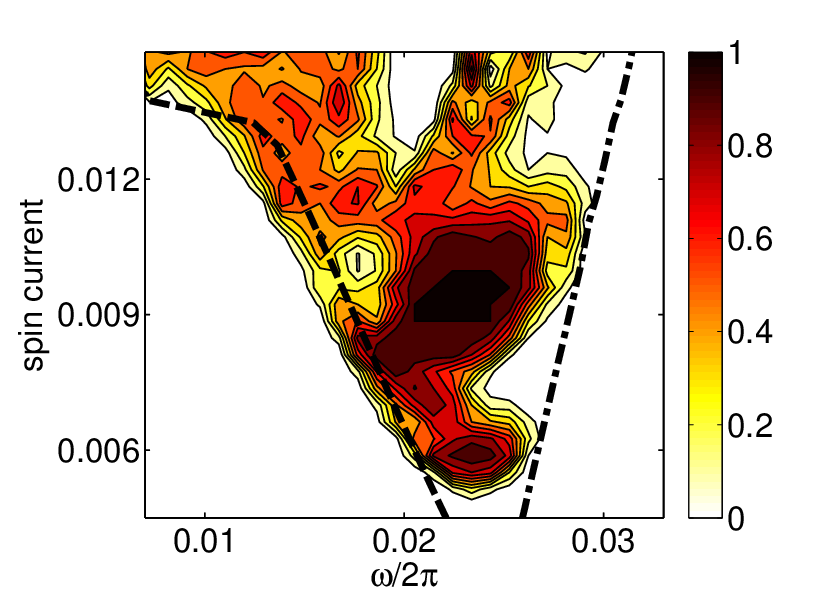
For the AC-perpendicular case Fig. 3 shows the switching probability as a function of spin current amplitude and AC frequency with the pulse duration of three oscillation periods , see also Fig. 5a. Notice that at optimal conditions the switching occurs at the current nearly two times lower than that in the DC perpendicular case with the switching currents as low as . One should also notice the sharp frequency selectivity of the switching process. The optimal AC frequency appears to be somewhat below the natural small precession frequency .
Simulations were also performed for pulses with different number of spin-current oscillations . For pulses with regions of low current switching were gradually excluded as approached until the switching probability was qualitatively the same as in the DC case of Fig. 2. For pulses with the range of currents and frequencies which produced switching remained qualitatively the same as in Fig. 3. However, the switching probabilities are reduced and oscillate with increasing reaching probability of 50% for sufficiently large values of . This behavior is the result of magnetization switching back and forth between the two minima with longer pulse times.

Fig. 4 shows the minimal Joule heat lost during the switch as a function of the spin current magnitude for both the DC and AC perpendicular cases. It is calculated by numerically integrating the power over time , where is a resistance which we assume to be constant through the switching process. For both AC and DC cases only combinations of spin current and AC frequency which result in switching probabilities above were are displayed. Notice the AC perpendicular method cost significantly less energy to produce switching at low spin current strengths. At its most energy efficient point the AC perpendicular method costs nearly one half the energy of the the most energy efficient DC perpendicular method. This point occurs at driving frequency , spin current amplitude , and the pulse duration of .
III Analytical considerations
We look now for a qualitative understanding of why the AC protocol requires a significantly smaller critical spin current. Another feature calling for an explanation is a sharp frequency dependence of the switching efficiency seen in Fig. 3. Figure 5a shows the AC spin torque pulse and the time dependence of the energy along a switching trajectory. Notice that the energy increases up to a bit over the top of the energy barrier during the time of the AC pulse and later decreases down to zero in the state with the reversed magnetization. Notice also that the energy is a rather smooth function of time. On the other hand the magnetization , depicted in Fig. 5b, goes through three full revolutions before the switching, exhibiting highly non-monotonic behavior.

This observation suggests to parameterize the magnetization vector in terms of a slow variable , which is nothing more than the energy of the free layer given by equation (4), and a fast variable which runs along a closed SW orbit of a constant energy. It is convenient to make the latter linearly related to the physical time (in the absence of the spin-torque). To this end we identify with the normalized time required to reach a given point along SW orbit within the purely conservative evolution, i.e. if (we omit the thermal stochastic noise (5) throughout this section). With this choice one takes , where, cf. Eq. (2),
| (6) |
and is the frequency of SW orbit, given by , where the integral runs along the SW orbit with energy and is given by Eq. (6). This defines the local parametrization , which may be shown [30] to be implicitly specified by its partial derivatives:
| (7) |
Notice that the parametrization is locally orthogonal, i.e. . One can thus project the identity onto these two orthogonal directions and employ LLG equation (1) for to find equations of motion for and pair
| (8) | |||||
| (9) |
Here the right hand sides may be also expressed as functions of and . The energy evolution is driven only by relatively weak damping and spin-torque terms, making the energy a slow variable. On the other hand, the phase dynamics is primarily given by a large , coming from LL term and making the phase the fast variable.
In presence of near resonant AC spin-torque the fast rotation phase tends to follow the external drive, see Fig. 5. One can thus introduce the relative phase as another slow variable. The equation of motion for the slow phase follows trivially from Eq. (9) and the relation
| (10) |
One can now employ the fact that both and change relatively little through one precession cycle to average over the fast precessing variable [17, 32]. To this end we write the AC spin current as and integrate the right hand sides of Eqs. (8), (10) over with the help of Eq. (6). This way we arrive at the pair of equations of motion for the slow degrees of freedom
| (11) |
Here the generalized forces averaged over the orbit with energy are given by
| (12) | |||||
where in the last two expressions we used the parity with respect to to single out odd and even components. It is worth noting here that the contribution to the spin current averages to zero upon this procedure.

A typical parametric trajectory versus is shown in figure (6) for a subcritical spin current. Notice that after averaging over the fast fluctuations and behave similarly to coordinate/momentum pair of an underdamped oscillator. The oscillation frequency of this effective oscillator is much smaller than the precession frequency and is rather given by . Of particular importance is the fact that before winding down into the stationary point (), the energy highly overshoots its equilibrium value. Had the energy exceeded the height of the energy barrier in the course of such an overshoot – a switch is likely to occur. This remains to be the case even if the equilibrium value is still below the barrier height . This is the qualitative reason for the AC critical current being significantly smaller than the DC one.
To make progress in explaining sharp frequency dependence of the effect, one needs to look closely at the equilibrium point () of the effective oscillator. Such a point would be reached by the free layer magnetization upon continuous AC drive with the amplitude below the switching one after all transients decay due to dissipation. Setting the left hand sides of equations (11) to zero gives such equilibrium conditions
| (13) |
Figure 7 shows the equilibrium energy over a range of frequencies along with simulated result found by adiabatically varying over time. Notice that for the range of frequencies there are two stable solutions and an unstable branch in between. Consequently the simulation reveal hysteretic loop with two jump frequencies, where the equilibrium energy abruptly jumps to a higher or lower value. Since the goal is to reach the switching energy , one wants to insure that the oscillator follows the upper of the two branches, while having as large equilibrium energy as possible. As seen from Fig. 7 this is achieved at frequencies right above the upper hysteresis jump . We thus calculate the upper jump frequency of the hysteresis as a function of the spin current and plot in Fig. 9.

To find a critical current of the swing switching it is useful to notice that in the absence of the dissipation , the AC spin-torque driven oscillator (11) possesses an integral of motion. Indeed, one may check that the following function
| (14) |
is conserved by the equations of motion (11), with , if the function is a solution of the following linear homogeneous differential equation:
| (15) |
In fact one may define the action , such that the change of variables in Eq. (14) results in the Hamiltonian written in terms of the canonical action-angle pair. The equations of motions (11) are nothing but the Hamilton equations: and .

The consequence of this observation is that without the dissipation the trajectories are closed. The corresponding phase portraits are are plotted in Fig. 8a,b for the case of and , correspondingly. There are two stable points and in the former case and only one in the latter. Hereafter we focus on the latter case, since for the former the evolution starting from can only bring the system to a small energy fixed point and thus is not beneficial for the switching. Starting from a vicinity of line the system evolves along a trajectory which is close to the separatrix line , before winding down towards the fixed point due to dissipation. For the switching to take place one must require that the separatrix goes beyond the top of the barrier . Since the maximum extent of the separatrix is reached at , a necessary condition for switching to occur is:
| (16) |
In fact this is an underestimate, since it does not take into account the dissipation. The latter dictates that the separatrix must exceed , where is the work done by the dissipative force along the separatrix trajectory. One can now substitute , where is found from the separatrix equation , to find the dissipative loss . One then uses instead of in Eq. (16) to obtain the minimal switching current. The resulting critical line is plotted in Fig. 9. One can see that this line is indeed close to the boundary of the observed switching range.
To make the general theory more transparent it is useful to evaluate the averaged generalized forces (12) at small energy . In this limits SW orbits are elliptical and the integrals in Eqs. (12) may be easily performed, leading to
| (17) | |||||
where
and . We have checked numerically that these expressions remain almost quantitatively correct in the entire relevant range of parameters. With these forces one finds , where is eccentricity index which ranges from in the absence of the easy plane anisotropy to in the strong easy plane case .
With these approximations the top of the separatrix line, given by the conditions and , is found from the cubic equation for , cf. Eq. (14),
| (18) |
It may have either three or one solution with the bifurcation point determining the relation. The critical current (16) is then found by the substitution of in the left hand side of Eq. (18). This way one finds an approximate location of the two lines depicted in Fig. 9. Their intersection results in the theoretical lower boundary for swing-switching critical current, which happens to be practically -independent for
| (19) |
One may notice that in our simulations the critical switching current is about factor of larger than this idealized estimate. The reason is that the estimate based on the conserved quantity (14) neglects the dissipation. Calculating the work of the friction force as described below Eq. (16), one finds with the proportionality coefficient which logarithmically diverges at (indeed, at the bifurcation point the dissipation always prevents the switching). In practice we found from the simulations that the condition
| (20) |
provides a good estimate for the underdamped range (). If one expects to approach the theoretical boundary (19). In the opposite case the AC perpendicular method losses its advantage over the DC approach, because the effective oscillator is overdamped.

One may notice that the simulations discussed above happen to have a mediocre quality factor , which may explain why they result in the critical current which is bigger than the theoretical bound (19). To test these predictions we performed additional simulations. Figure 10 shows for , , and . Notice that for is overdamped and for is highly underdamped. Notice also that in the underdamped case the maximum energy is significantly higher than in the other two. Expanding this analysis further Fig. 11 shows the maximum transient energy as a function of for several values of . To keep constant we adjusted dissipation according to Eq. (20), while and are kept fixed and . Notice that the maximal energy remains almost completely constant for each value of and grows with increasing , so that for the maximum energy is nearly larger than for . This shows that, if the spin-current is scaled with and AC frequency is scaled with , the system behavior is governed by the single scaling parameter , defined in Eq. (20). This observation reduces the multidimensional space of system’s parameters down to the single essential parameter: the quality factor .
For cases where the effectiveness of the AC-perpendicular method is diminished in comparison to the equivalent DC method. This is the result of higher energy trajectories, , spending more time at larger values of azimuthal angle . This causes the contribution to the ST in the DC case to become stronger than the contribution to the ST in the AC case. A more detailed description of this effect is left for future works.

IV Conclusion
We have shown that by using an AC spin current with driving frequency close to the precession frequency of the free layer one may achieve the reliable switching of spin-torque valves. Keeping advantages of the DC perpendicular approach [13, 14, 21, 22], the switching times are well below . In addition, the AC method offers a significant reduction of the critical switching current and associated energy dissipation. We explained the effect by the underdamped nature of the effective non-linear oscillator, which allows to cross the energy barrier by transient oscillations. The latter may significantly overshoot the equilibrium energy, reducing the spin-torque required for the switch to occur.
We have developed a theoretical description of the effect which allowed us to identify the optimal AC frequency with the upper bifurcation frequency of the driven non-linear oscillator. It also provides with the estimate of the current amplitude needed to perform the switch. Possibly most essentially, it provides the scaling arguments showing that ; , while the relative advantage of the AC method is governed by the single scaling parameter: the quality factor , Eq. (20).
We would like to thank Alex Chudnovskiy for enlightening discussions. This work was supported by NSF Grant DMR-0804266 and U.S.-Israel Binational Science Foundation Grant 2008075.
References
- [1] J. C. Slonczewski, J. Magn. Magn. Mater. 159, L1 (1996).
- [2] L. Berger, Phys. Rev. B 54, 9353 (1996).
- [3] E. B. Myers, D. C. Ralph, J. A. Katine, R. N. Louie, and R. A. Buhrman, Science 285, 867 (1999).
- [4] J. A. Katine, F. J. Albert, R. A. Buhrman, E. B. Myers, and D. C. Ralph, Phys. Rev. Lett. 84, 3149 (2000).
- [5] M. Hosomi, H. Yamagishi, T. Yamamoto, K. Bessho, Y. Higo, K. Yamane, H. Yamada, M. Shoji, H. Hachino, C. Fukumoto, et al., in Electron Devices Meeting, 2005. IEDM Technical Digest. IEEE International (2005), pp. 459 –462.
- [6] S. Matsunaga, K. Hiyama, A. Matsumoto, S. Ikeda, H. Hasegawa, K. Miura, J. Hayakawa, T. Endoh, H. Ohno, and T. Hanyu, Applied Physics Express 2, 023004 (2009).
- [7] J. Grollier, V. Cros, A. Hamzic, J. M. George, H. Jaffres, A. Fert, G. Faini, J. B. Youssef, and H. Legall, Appl. Phys. Lett. 78, 3663 (2001).
- [8] B. Ozyilmaz, A. D. Kent, D. Monsma, J. Z. Sun, M. J. Rooks, and R. H. Koch, Phys. Rev. Lett. 91, 067203 (2003).
- [9] S. Urazhdin, N. O.Birge, W. P. Pratt, and J. Bass, Phys. Rev. Lett. 91, 146803 (2003).
- [10] T. Seki, S. Mitani, K. Yakushiji, and K. Takanashi, Appl. Phys. Lett. 88, 172504 (2006).
- [11] S. Yuasa and D. D. Djayaprawira, J. Phys. D: Appl. Phys. 40, R337 (2007).
- [12] J. Z. Sun, Phys. Rev. B. 62, 570 (2000).
- [13] O. J. Lee, V. S. Pribiag, P. M. Braganca, P. G. Gowtham, D. C. Ralph, and R. A. Buhrman, Appl. Phys. Lett. 95, 012506 (2009).
- [14] D. E. Nikonov, G. I. Bourianoff, G. Rowlands, and I. N. Krivorotov, J. Appl. Phys. 107, 113910 (2010).
- [15] E. B. Myers, F. J. Albert, J. C. Sankey, E. Bonet, R. A. Buhrman, and D. C. Ralph, Phys. Rev. Lett. 89, 196801 (2002).
- [16] Z. Li and S. Zhang, Phys. Rev. B 70, 024417 (2004).
- [17] D. M. Apalkov and P. B. Visscher, Phys. Rev. B 72, 180405(R) (2005).
- [18] D. Bedau, H. Liu, J.-J. Bouzaglou, A. D. Kent, J. Z. Sun, J. A. Katine, E. E. Fullerton, and S. Mangin, Appl. Phys. Lett. 96, 022514 (2010).
- [19] T. Dunn and A. Kamenev, Appl. Phys. Lett. 98, 143109 (2011).
- [20] A. D. Kent, B. Özyilmaz, and E. del Barco, Appl. Phys. Lett. 84, 3897 (2004).
- [21] H. Liu, D. Bedau, D. Backes, J. A. Katine, J. Langer, and A. D. Kent, Appl. Phys. Lett. 97, 242510 (2010).
- [22] G. E. Rowlands, T. Rahman, J. A. Katine, J. Langer, A. Lyle, H. Zhao, J. G. Alzate, A. A. Kovaley, Y. Tserkovnyak, Z. M. Zeng, et al., Appl. Phys. Lett. 98, 102509 (2011).
- [23] J. C. Sankey, P. M. Braganca, A. G. F. Garcia, I. N. Krivorotov, R. A. Buhrman, and D. C. Ralph, Phys. Rev. Lett 96, 227601 (2006).
- [24] A. Mourachkine, O. V. Yazyev, C. Ducati, and J. P. Ansermet, Nano Lett 8, 3683 (2008).
- [25] A. A. Tulapurkar, Y. Suzuki, A. Fukushima, H. Kubota, H. Maehara, K. Tsunekawa, D. D. Djayaprawira, N. Watanabe, and S. Yuasa, Nature 438, 339 (2005).
- [26] B. Georges, J. Grollier, V. Cros, A. Fert, A. Fukushima, H. Kubota, K. Yakushijin, S. Yuasa, and K. Ando, App. Phys. Expr. 2, 123003 (2009).
- [27] D. E. Nikonov, G. I. Bourianoff, G. Rowlands, and I. N. Krivorotov, Phys. Rev. B 78, 184403 (2008).
- [28] X. Cheng, C. T. Boone, J. Zhu, and I. N. Krivorotov, Phys. Rev. Lett. 105 (2010).
- [29] Y. T. Cui, J. C. Sankey, C. Wang, K. V. Thadani, Z. P. Li, R. A. Buhrman, and D. C. Ralph, Phys. Rev. B 77, 214440 (2008).
- [30] T. Dunn, A. Chudnovskiy, and A. Kamenev, in Fluctuating Nonlinear Oscillators (2012), pp. 142 –164.
- [31] W. F. Brown, Phys. Rev. 130, 1677 (1963).
- [32] M. I. Dykman and M. A. Krivoglaz, JETP 50, 30 (1979).
- [33] J. Swiebodzinski, A. Chudnovskiy, T. Dunn, and A. Kamenev, Phys. Rev. B. 82, 144404 (2010).