Minimally Infrequent Itemset Mining using Pattern-Growth Paradigm and Residual Trees
Abstract
Itemset mining has been an active area of research due to its successful
application in various data mining scenarios including finding association
rules. Though most of the past work has been on finding frequent itemsets,
infrequent itemset mining has demonstrated its utility in web mining,
bioinformatics and other fields. In this paper, we propose a new algorithm
based on the pattern-growth paradigm to find minimally infrequent itemsets.
A minimally infrequent itemset has no subset which is also infrequent. We
also introduce the novel concept of residual trees. We further utilize the
residual trees to mine multiple level minimum support itemsets where
different thresholds are used for finding frequent itemsets for different
lengths of the itemset. Finally, we analyze the behavior of our algorithm
with respect to different parameters and show through experiments that it
outperforms the competing ones.
Keywords: Itemset Mining, Minimal Infrequent Itemsets, Residual Tree, Projected Tree.
1 Introduction
Mining frequent itemsets has found extensive utilization in various data mining applications including consumer market-basket analysis [1], inference of patterns from web page access logs [11], and iceberg-cube computation [2]. Extensive research has, therefore, been conducted in finding efficient algorithms for frequent itemset mining, especially in finding association rules [3].
However, significantly less attention has been paid to mining of infrequent itemsets, even though it has got important usage in (i) mining of negative association rules from infrequent itemsets [12], (ii) statistical disclosure risk assessment where rare patterns in anonymous census data can lead to statistical disclosure [7], (iii) fraud detection where rare patterns in financial or tax data may suggest unusual activity associated with fraudulent behavior [7], and (iv) bioinformatics where rare patterns in microarray data may suggest genetic disorders [7].
The large body of frequent itemset mining algorithms can be broadly classified into two categories: (i) candidate generation-and-test paradigm and (ii) pattern-growth paradigm. In earlier studies, it has been shown experimentally that pattern-growth based algorithms are computationally faster on dense datasets.
Hence, in this paper, we leverage the pattern-growth paradigm to propose an algorithm IFP_min for mining minimally infrequent itemsets. For some datasets, the set of infrequent itemsets can be exponentially large. Reporting an infrequent itemset which has an infrequent proper subset is redundant, since the former can be deduced from the latter. Hence, it is essential to report only the minimally infrequent itemsets.
Haglin et al. proposed an algorithm, MINIT, to mine minimally infrequent itemsets [7]. It generated all potential candidate minimal infrequent itemsets using a ranking order of the items based on their supports and then validated them against the entire database.
Instead, our proposed IFP_min algorithm proceeds by processing minimally infrequent itemsets by partitioning the dataset into two parts, one containing a particular item and the other that does not.
If the support threshold is too high, then less number of frequent itemsets will be generated resulting in loss of valuable association rules. On the other hand, when the support threshold is too low, a large number of frequent itemsets and consequently large number of association rules are generated, thereby making it difficult for the user to choose the important ones. Part of the problem lies in the fact that a single threshold is used for generating frequent itemsets irrespective of the length of the itemset. To alleviate this problem, Multiple Level Minimum Support (MLMS) model was proposed [5], where separate thresholds are assigned to itemsets of different sizes in order to constrain the number of frequent itemsets mined. This model finds extensive applications in market basket analysis [5] for optimizing the number of association rules generated. We extend our IFP_min algorithm to the MLMS framework as well.
In summary, we make the following contributions:
-
We propose a new algorithm IFP_min for mining minimally infrequent itemsets. To the best of our knowledge, this is the first such algorithm based on pattern-growth paradigm (Section 5).
-
We introduce the concept of residual trees using a variant of the FP-tree structure termed as inverse FP-tree (Section 4).
-
We propose an optimization on the Apriori algorithm to mine minimally infrequent itemsets (Section 5.4).
-
We present a detailed study to quantify the impact of variation in the density of datasets on the computation time of Apriori, MINIT and our algorithm.
-
We extend the proposed algorithm to mine frequent itemsets in the MLMS framework (Section 6).
| Tid | Transactions |
|---|---|
| T1 | F, E |
| T2 | A, B, C |
| T3 | A, B |
| T4 | A, D |
| T5 | A, C, D |
| T6 | B, C, D |
| T7 | E, B |
| T8 | E, C |
| T9 | E, D |
1.1 Problem Specification
Consider to be a set of items. An itemset is a subset of items. If its length or cardinality is , it is referred to as a k-itemset. A transaction is a tuple where is the transaction identifier and is an itemset. It is said to contain an itemset if and only if . A transaction database is simply a set of transactions.
Each itemset has an associated statistical measure called support. For an itemset , where is the number of transactions in that contains . For a user defined threshold , an itemset is frequent if and only if its support is greater than or equal to . It is infrequent otherwise.
As mentioned earlier, the number of infrequent itemsets for a particular database may be quite large. It may be impractical to generate and report all of them. A key observation here is the fact that if an itemset is infrequent, so will be all its supersets. Thus, it makes sense to generate only minimal infrequent itemsets, i.e., those which are infrequent but whose all subsets are frequent.
Definition 1 (Minimally Infrequent Itemset).
An itemset is said to be minimally infrequent for a support threshold if it is infrequent and all its proper subsets are frequent, i.e., and .
Given a particular support threshold, our goal is to efficiently generate all the minimally infrequent itemsets (MIIs) using the pattern-growth paradigm.
Consider an example transaction database shown in Table 1. If , is one of the minimally infrequent itemsets for the transaction database. All its subsets, i.e., and , are frequent but it itself is infrequent as its support is . The whole set of MIIs for the transaction database is , , , , , , , . Note that is not a MII since one of its subsets is infrequent as well.
In the MLMS framework, the problem is to find all frequent (equivalently, infrequent) itemsets with different support thresholds assigned to itemsets of different lengths. We define as the minimum support threshold for a k-itemset () to be frequent. A k-itemset is frequent if and only if .
For efficient processing of MLMS itemsets, it is useful to sort the list of items in each transaction in increasing order of their support counts. This is called the i-flist order. Also, let be lowest minimum support threshold.
Most applications use the constraint . This is intuitive as the support of larger itemsets can only decrease or at most remain constant. In this case, . Our algorithm IFP_MLMS, however, does not depend on this assumption, and works for any general .
Consider an example transaction database shown in Table 2. The frequent itemsets corresponding to the different thresholds are shown in Table 3.
| Tid | Transactions | Items in i-flist order |
|---|---|---|
| T1 | A, C, T, W | A, T, W, C |
| T2 | C, D, W | D, W, C |
| T3 | A, C, T, W | A, T, W, C |
| T4 | A, D, C, W | A, D, W, C |
| T5 | A, T, C, W, D | A, D, T, W, |
| T6 | C, D, T, B | B, D, T, C |
| Frequent k-itemsets | |
|---|---|
| {C}, {W}, {T}, {D}, {A} | |
| {C, D}, {C, W}, {C, A}, {W, A}, {C, T} | |
| {C, W, T}, {C, W, D}, {C, W, A}, | |
| {C, T, A}, {W, T, A} | |
| {C, W, T, A}, {C, D, W, A} | |
| {C, W, T, D, A} |
2 Related Work
The problem of mining frequent itemsets was first introduced by Agrawal et al. [1], who proposed the Apriori-algorithm. Apriori is a bottom-up, breadth-first search algorithm that exploits the downward closure property “all subsets of frequent itemsets are frequent”. Only candidate frequent itemsets whose subsets are all frequent are generated in each database scan. Apriori needs database scans if the size of the largest frequent itemset is . In this paper, we propose a variation of the Apriori algorithm for mining minimally infrequent itemsets (MIIs).
In [8], Han et al. introduced a novel algorithm known as the FP-growth method for mining frequent itemsets. The FP-growth method is a depth-first search algorithm. A data structure called the FP-tree is used for storing the frequency information of itemsets in the original transaction database in a compressed form. Only two database scans are needed for the algorithm and no candidate generation is required. This makes the FP-growth method much faster than Apriori. In [6], Grahne et al. introduced a novel FP-array technique that greatly reduces the need to traverse the FP-trees. In this paper, we use a variation of the FP-tree for mining the MIIs.
To the best of our knowledge there has been only one other work that discusses the mining of MIIs. In [7], Haglin et al. proposed the algorithm MINIT which is based upon the SUDA2 algorithm developed for finding unique itemsets (itemsets with no unique proper subsets) [9, 10]. The authors also showed that the minimal infrequent itemset problem is NP-complete [7].
In [5], Dong et al. proposed the MLMS model for constraining the number of frequent and infrequent itemsets generated. A candidate generation-and-test based algorithm Apriori_MLMS was proposed in [5]. The downward closure property is absent in the MLMS model, and thus, the Apriori_MLMS algorithm checks the supports of all possible k-itemsets occurring at least once in the transaction database, for finding the frequent itemsets. Generally, the support thresholds are chosen randomly for different length itemsets with the constraint . In [4], Dong et al. extended their proposed algorithm from [5] to include an interestingness parameter while mining frequent and infrequent itemsets.
3 Need for Residual Trees
By definition, an itemset is a minimally infrequent itemset (MII) if and only if it is infrequent and all its subsets are frequent. Thus, a trivial algorithm to mine all MIIs would be to compute all the subsets for every infrequent itemset and check if they are frequent. This involves finding all the frequent and infrequent itemsets in the database and proceeding with checking the subsets of infrequent itemsets for occurrence in the large set of frequent itemsets. This is a simple but computationally expensive algorithm.
The use of residual trees reduces the computation time. A residual tree for a particular item is a tree representation of the residual database corresponding to the item, i.e., the entire database with the item removed. We show later that a MII found in the residual tree is a MII of the entire transaction database.
The projected database, on the other hand, corresponds to the set of transactions that contains a particular item. A potential minimal infrequent itemset mined from the projected tree must not have any infrequent subset. The itemset itself is a subset since it is actually the union with the item of the projected tree that is under consideration. As we show later, the support of only this itemset needs to be computed from the corresponding residual tree.
In this paper, our proposed algorithm IFP_min uses a structure similar to the FP-tree [8] called the IFP-tree. This is due to the fact that the IFP-tree provides a more visually simplified version of the residual and projected trees that leads to enhanced understanding of the algorithm. A similar algorithm FP_min can be designed that uses the FP-tree. The time complexity remains the same. In the next section, we describe in detail the IFP-tree and the corresponding structures, projected tree and residual tree.
4 Inverse FP-tree (IFP-tree)
The inverse FP-tree (IFP-tree) is a variant of the FP-tree [8]. It is a compressed representation of the whole transaction database. Every path from the root to a node represents a transaction. The root has an empty label. Except the root node, each node of the tree contains four fields: (i) item id, (ii) count, (iii) list of child links, and (iv) a node link. The item id field contains the identifier of the item. The count field at each node stores the support count of the path from the root to that node. The list of child links point to the children of the node. The node link field points to another node with the same item id that is present in some other branch of the tree.
An item header table is used to facilitate the traversal of the tree. The header table consists of items and a link field associated with each item that points to the first occurrence of the item in the IFP-tree. All link entries of the header table are initially set to null. Whenever an item is added into the tree, the corresponding link entry of the header table is updated. Items in each transaction are sorted according to their order in i-flist.
For inserting a transaction, a path that shares the same prefix is searched. If there exists such a path, then the count of the common prefix is incremented by one in the tree and the remaining items of the transaction (which do not share the path) are attached from the last node with their count value set to . If items of a transaction do not share any path in the tree, then they are attached from the root. The IFP-tree for the sample transaction database in Table 1 (considering only the transactions T2 to T9) is shown in Figure 1.

The IFP_min algorithm recursively mines the minimally infrequent itemsets (MIIs) by dividing the IFP-tree into two sub-trees: projected tree and residual tree. The next two sections describe them.
4.1 Projected Tree
Suppose be the transaction database represented by the IFP-tree and denotes the database of transactions that contain the item . The projected database corresponding to the item is the database of these transactions , but after removing the item from the transactions. The IFP-tree corresponding to this database is called the projected tree of item in . Figure 2a shows the projected tree of item , which is the least frequent item in Figure 1.
The IFP_min algorithm considers the projected tree of only the least frequent item (lf-item). Henceforth, for simplicity, we associate every IFP-tree with only a single projected tree which is that of the lf-item. Moreover, since the items are sorted in the i-flist order, there would be a single node of the lf-item in the IFP-tree. Thus, the projected tree of can be obtained directly from the IFP-tree by considering the subtree rooted at node .
4.2 Residual Tree
The residual database corresponding to an item is the database of transactions obtained by removing item from . The IFP-tree corresponding to this database is called residual tree of item in . Figure 2b shows the residual tree of the least frequent item . It is obtained by deleting the node corresponding to item and then merging the subtree below that node into the main tree at appropriate positions.
Similar to the projected tree, the IFP_min algorithm considers the residual tree of only the lf-item. Since there is only a single node of the lf-item in the IFP-tree, the residual tree of can be obtained directly from the IFP-tree by deleting the node from the tree and then merging the subtree below the node with the rest of the tree.
Furthermore, the projected and residual tree of the next item (i.e., ) in the i-flist is associated with the residual tree of the current item (i.e., ). Figure 3 shows the projected and residual trees of the item for the tree .


5 Mining Minimally Infrequent Itemsets
In this section, we describe the IFP_min algorithm that uses a recursive approach to mine minimally infrequent itemsets (MIIs). The steps of the algorithm are shown in Algorithm 1.
The algorithm uses a dot-operation () that is used to unify sets. The unification of the first set with the second produces another set whose element is the union of the entire first set with the element of the second set. Mathematically, and .
The infrequent 1-itemsets are trivial MIIs and so they are reported and pruned from the database in Step 1. After this step, all the items present in the modified database are individually frequent. IFP_min then selects the least frequent item (lf-item, Step 3) and divides the database into two non-disjoint sets: projected database and residual database of the lf-item (Step 11 and Step 12 respectively).
The IFP_min algorithm is then applied to the residual database in Step 13 and the corresponding MIIs are reported in Step 14. In the base case (Step 6 to Step 12) when the residual database consists of a single item, the MII reported is either the item itself or the empty set accordingly as the item is infrequent or frequent respectively.
After processing the residual database, the algorithm mines the projected database in Step 15. The itemsets in the projected database share the lf-item as a prefix. The MIIs obtained from the projected database by recursively applying the algorithm are compared with those obtained from residual database. If an itemset is found to occur in the second set, it is not reported; otherwise, the lf-item is included in the itemset and is reported as an MII of the original database (Step 16).
IFP_min also reports the 2-itemsets consisting of the lf-item and frequent items not present in the projected database of the lf-item (Step 17). These 2-itemsets have support zero in the actual database and hence also qualify as MIIs.
5.1 Example
Consider the transaction database shown in Table 1. Figure 4 shows the recursive partitioning of the tree corresponding to . The box associated with each tree represents the MIIs in that tree for .
The algorithm starts by separating the infrequent items from the database. This results in removal of the item (which is inherently a MII). The lf-item in the modified tree is . The algorithm then constructs the projected tree and the residual tree corresponding to item and recursively processes them to yield MIIs containing and MIIs not containing respectively.
-
MIIs not containing (itemsets obtained from )
The lf-item in is . Therefore, similar to the first step, is again divided into projected tree and residual tree , which are then recursively mined.
-
MIIs not containing (itemsets obtained from )
Every 1-itemset is frequent. By recursively processing the residual and projected trees of , is obtained as a MII. Itemset is also obtained as a potential MII. However, since it is frequent, it is not returned. Since is also frequent, only is returned from this tree.
-
MIIs containing (itemsets obtained from )
All the 1-itemsets are infrequent (Step 6 of the algorithm). is included with these itemsets to return .
and are mutually exclusive. Hence, the combined set forms the MIIs not containing .
-
-
MIIs containing (itemsets obtained from )
Item is infrequent (). Hence, forms a MII. Similarly, itemset with is also obtained as a potential MII. The other MIIs obtained from recursive processing are . The itemset , however, appears as a MII in both and . Hence, it is removed (Step 16 of the algorithm). This avoids the inclusion of the itemset which is not a MII since is infrequent (as shown in ). is included with the remaining set of MIIs from to form the itemsets .
The combined set thus forms the MIIs containing .
As mentioned in Step 3 of the algorithm, the infrequent 1-itemset is also included. Hence, in all, the algorithm returns the set as the MIIs for the database .

5.2 Completeness and Soundness
In this section, we prove formally the our algorithm is complete and sound, i.e., it returns all minimally infrequent itemsets and all itemsets returned by it are minimally infrequent.
Consider the lf-item in the transaction database. MIIs in the database can be exhaustively divided into the following sets:
-
Group 1: MIIs not containing
This can be again of two kinds:
- (a)
Itemsets of length 1:
These constitute the infrequent items in the database obtained from the initial pruning.
- (b)
Itemsets of length greater than 1:
These constitute the minimally infrequent itemsets obtained from the residual tree of .
- (a)
-
Group 2: MIIs containing
This consists of itemsets of the form where can be of following two kinds:
- (a)
occurs with in at least one transaction:
All items in occur in the projected tree of .
- (b)
does not occur with in any transaction:
Note that the path corresponding to does not exist in the projected tree of . Also, is a 1-itemset. Assume the contrary, i.e., contains two or more items. A subset of would then exist, which would not occur with in any transaction. As a result, the subset would also be infrequent and would not be qualified as a MII. Thus, is a node that is absent in the projected tree of .
- (a)
The following set of observations and theorems prove the correctness of the IFP_min algorithm. They exhaustively define and verify the set of itemsets returned by the algorithm.
The first observation relates the (in)frequent itemsets of the database to those present in the residual database.
Observation 1.
An itemset (not containing the item ) is frequent (infrequent) in the residual tree if and only if the itemset is frequent (infrequent) in , i.e.,
is frequent in is frequent in ()
is infrequent in is infrequent in ()
Proof.
Since does not contain , it does not occur in the projected tree of . All occurrences of must, therefore, be only in the residual tree , i.e.,
| (1) |
Hence, is frequent (infrequent) in if and only if is frequent (infrequent) in . ∎
The following theorem shows that the MIIs that do not contain the item can be obtained directly as MIIs from the residual tree of .
Theorem 1.
An itemset (not containing the item ) is minimally infrequent in if and only if the itemset is minimally infrequent in the residual tree of , i.e.,
is minimally infrequent in
is minimally infrequent in ()
Proof.
Suppose is minimally infrequent in . Therefore, it is itself infrequent, but all its subsets are frequent.
As does not contain , all occurrences of or any of its subsets must occur in the residual tree only. Hence, using Observation 1, in also, is infrequent but all are frequent. Therefore, is minimally infrequent in as well.
The converse is also true, i.e., if is minimally infrequent in , since all its occurrences are in only, it is globally minimally infrequent (i.e., in ) as well. ∎
Theorem 1 guides the algorithm in mining MIIs not containing the least frequent item (lf-item) . The algorithm makes use of this theorem recursively, by reporting MIIs of residual trees as MIIs of the original tree. For mining of MIIs that contain , the following observation and theorem are presented.
The second observation relates the (in)frequent itemsets of the database to those present in the projected database.
Observation 2.
An itemset is frequent (infrequent) in the projected tree if and only if the itemset obtained by including in (i.e., ), is frequent (infrequent) in , i.e.,
is frequent in is frequent in
is infrequent in is infrequent in
Proof.
Consider the itemset . All occurrences of it are only in the projected tree . The projected tree, however, does not list , and therefore, we have,
| (2) |
Hence, is frequent (infrequent) in if and only if is frequent (infrequent) in . ∎
The next theorem shows that the potential MIIs obtained from the projected tree of an item (by appending to it) is a MII provided it is not a MII in the corresponding residual tree of .
Theorem 2.
An itemset is minimally infrequent in if and only if the itemset is minimally infrequent in the projected tree but not minimally infrequent in the residual tree , i.e.,
is minimally infrequent in
is minimally infrequent in and
is not minimally infrequent in
Proof.
LHS to RHS:
Suppose is minimally infrequent in . Therefore, it is itself infrequent, but all its subsets , including , are frequent.
Since is frequent and it does not contain , using Observation 1, is frequent in and is, therefore, not minimally infrequent in .
From Observation 2, is infrequent in . Assume that is not minimally infrequent in . Since it is infrequent itself, there must exist a subset which is infrequent in as well. Now, consider the itemset . From Observation 2, it must be infrequent in . However, since this is a subset of , this contradicts the fact that is minimally infrequent. Therefore, the assumption that is not minimally infrequent in is false.
Together, it shows that if is minimally infrequent in , then is minimally infrequent in but not in .
RHS to LHS:
Given that is minimally infrequent in but not in , assume that is not minimally infrequent in . Since is infrequent in , using Observation 2, is also infrequent in .
Now, since we have assumed that is not minimally infrequent in , it must contain a subset which is infrequent in as well.
Suppose contains , i.e., . Consider the itemset such that . Note that since , . Since is infrequent in , from Observation 2, is infrequent in . However, since , this contradicts the fact that is minimally infrequent in . Hence, cannot contain .
Therefore, it must be the case that . To show that this leads to a contradiction as well, we first show that
Now, if is minimally infrequent in but not in and is not minimally infrequent in , then every subset is frequent in . Thus, is frequent in as well (since is only a part of ). Then, if is infrequent, it must be a MII. However, from Theorem 1, it becomes a MII in which is a contradiction. Therefore, cannot be infrequent and is, therefore, frequent in .
Since, but , therefore, . We have already shown that is infrequent in . Using the Apriori property, cannot then be frequent. Hence, it contradicts the original assumption that is not minimally infrequent in .
Together, we get that if is minimally infrequent in but not in , then is minimally infrequent in . ∎
Theorem 2 guides the algorithm in mining MIIs containing the least frequent item (lf-item) . The algorithm first obtains the MIIs from its projected tree and then removes those that are also found in the residual tree. It thus shows the connection between the two parts of the database, projected and residual.
5.3 Correctness
We now formally establish the correctness of the algorithm IFP_min by showing that the MIIs as enumerated in Group 1 and Group 2 in Section 5.2 are generated by it.
In Step 1, the algorithm first finds the infrequent items present in the tree. These 1-itemsets cover the Group 1(a).
Consider the least frequent item . In Step 11 and Step 12, the tree is divided into smaller trees, the residual tree and the projected tree .
In Step 13, Group 1(b) MIIs are obtained by the recursive application of IFP_min on the residual tree . Theorem 1 proves that these are MIIs in the original dataset.
In Step 14, potential MIIs are obtained by the recursive application of IFP_min on the projected tree . MIIs obtained from are removed from this set. Combined with the item , these form the MIIs enumerated as Group 2(a). Theorem 2 proves that these are indeed MIIs in the original dataset.
The projected database consist of all those transactions in which is present. The Group 2(b) MIIs are of length 2 (as shown earlier). Thus, single items that are frequent but do not appear in the projected tree of , when combined with , constitute MIIs with support count of zero. These items appear in though as they are frequent. Hence, they are obtained as single items that appear in but not in as shown in Step 17 of the algorithm.
The algorithm is, hence, complete and it exhaustively generates all minimally infrequent itemsets.
5.4 MIIs using Apriori
In this section, we show how the Apriori algorithm [1] can be improved to mine the MIIs. Consider the iteration where candidate itemsets of length are generated from frequent itemsets of length . From the generated candidate set, itemsets whose support satisfies the minimum support threshold are reported as frequent and the rest are rejected. This rejected set of itemsets constitute the MIIs of length . This is attributed to the fact that for such an itemset, all the subsets are frequent (due to the candidate generation procedure) while the itemset itself is infrequent. For the experimentation purposes, we label this algorithm as the Apriori_min algorithm.
6 Frequent Itemsets in MLMS Model
In this section, we present our proposed algorithm IFP_MLMS to mine frequent itemsets in the MLMS framework. Though most applications use the constraint for the different support thresholds at different lengths, our algorithm (shown in Algorithm 2) does not depend on it and works for any general .
We use the lowest support in the algorithm. The algorithm is based on the item with least support which we term as the ls-item.
IFP_MLMS is again based on the concepts of residual and projected trees. It mines the frequent itemsets by first dividing the database into projected and residual trees for the ls-item , and then mining them recursively. We show that the frequent itemsets obtained from the residual tree are frequent itemsets in the original database as well.
The itemsets obtained from the projected tree share the ls-item as a prefix. Hence, the thresholds cannot be applied directly as the length of the itemset changes. The prefix accumulates as the algorithm goes deeper into recursion, and hence, a track of the prefix is maintained at each recursion level. At any stage of the recursive processing, if -, then this item cannot occur in a frequent itemset of any length (as any superset of it will not pass the support threshold). Thus, its sub-tree is pruned, thereby reducing the search space considerably.
To analyze the prefix items corresponding to a tree, the following two definitions are required:
Definition 2 (Prefix-set of a tree).
The prefix-set of a tree is the set of items that need to be included with the itemsets in the tree, i.e., all the items on which the projections have been done. For a tree , it is denoted by .
Definition 3 (Prefix-length of a tree).
The prefix-length of a tree is the length of its prefix-set. For a tree , it is denoted by .
For a tree having and , the corresponding values for the residual tree are and while those for the projected tree are and . For the original transaction database and its tree , and .
For any -itemset in a tree , the original itemset must include all the items in the prefix-set. Therefore, if , for to be frequent, it must satisfy the support threshold for -length itemsets, i.e., (henceforth, is also used to denote ). The definitions of frequent and infrequent itemsets in a tree with a prefix-length are, thus, modified as follows.
Definition 4 (Frequent* itemset).
A k-itemset is frequent* in having if .
Definition 5 (Infrequent* itemset).
A k-itemset is infrequent* in having if .
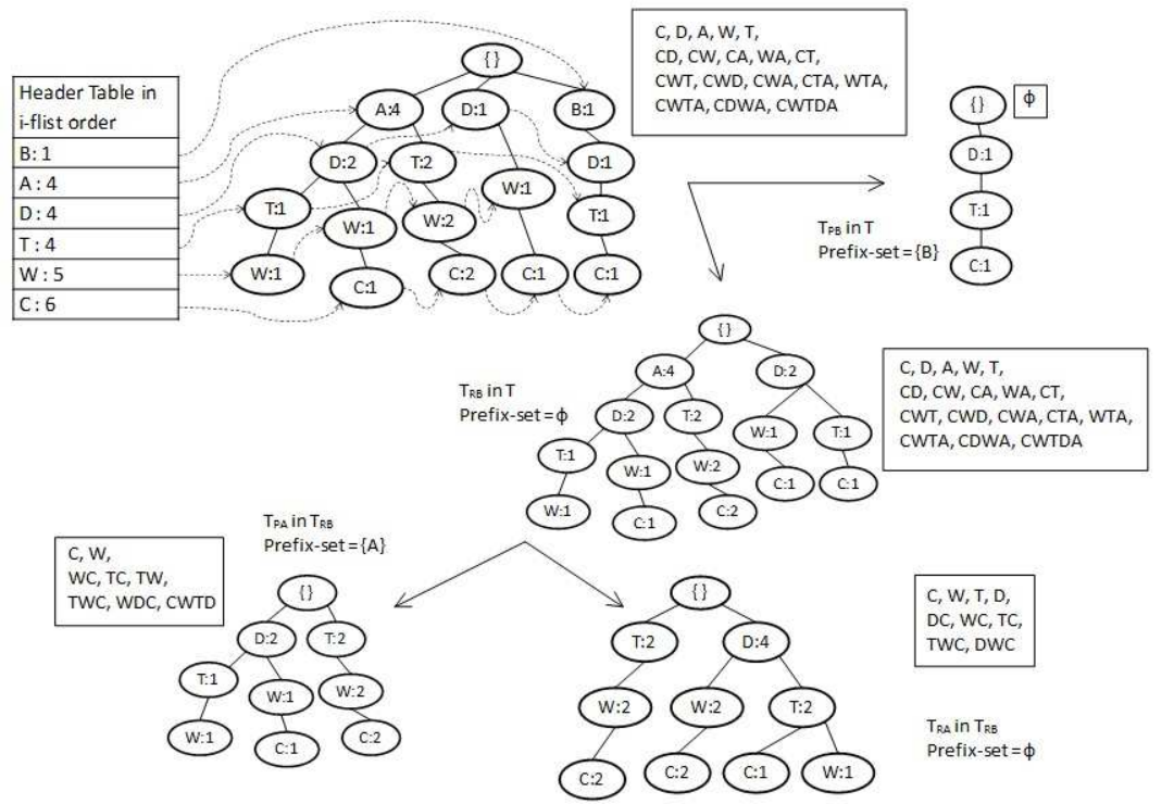
Using these definitions, we explain Algorithm 2 along with an example shown in Figure 5 for the database in Table 2. The support thresholds are , , , , and .
The item with least support for the initial tree is . Since its support is above (Step 5), the algorithm extracts the projected tree and then recursively processes it (Step 11 to Step 13).
The algorithm then processes the residual tree recursively (Step 12 to Step 14). For that, it breaks it into the projected and residual trees of the ls-item there, which is . Figure 5 shows all the frequent itemsets mined.
Since itself is not frequent in (Step 15), it is not returned. The other itemsets are returned (Step 18).
6.1 Correctness of IFP_MLMS
Let be the ls-item in tree (having ) and be a k-itemset not containing .
For computing the frequent* itemsets for a tree , the IFP_MLMS algorithm merges the frequent* itemsets, obtained by the processing of the projected tree and residual tree of ls-item, using the following theorem
Theorem 3.
An itemset is frequent* in if and only if is frequent* in the projected tree of , i.e.,
is frequent* in is frequent* in
Proof.
Suppose is a -itemset.
is frequent* in
(since
)
(using
Observation 2)
is frequent* in (since ).
∎
Theorem 4.
An itemset (not containing ) is frequent* in if and only if frequent* in the residual tree of , i.e.,
is frequent* in is frequent* in
Proof.
Suppose is a -itemset.
is frequent* in
(since )
(using
Observation 1)
is frequent* in (since ).
∎
The algorithm IFP_MLMS merges the following frequent* itemsets: (i) frequent* itemsets obtained by including with those returned from the projected tree (shown to be correct by Theorem 3), (ii) frequent* itemsets obtained from the residual tree (shown to be correct by Theorem 4) and (iii) 1-itemset if it is frequent* in . The root of the tree that represents the entire database has a null prefix-set, and therefore, zero prefix-length. Hence, all frequent* itemsets mined from that tree are the frequent itemsets in the original transaction database.
7 Experimental Results
In this section, we report the experimental results of running our algorithms on different datasets. We first report the performance of IFP_min algorithm in comparison with the Apriori_min and MINIT algorithms, followed by that of the IFP_MLMS algorithm. The benchmark datasets have been taken from Frequent Itemset Mining Implementations (FIMI) repository http://fimi.ua.ac.be/data/. All experiments were run on a machine with Dual Core Intel Processor running at 2.4GHz with 8GB of RAM.
7.1 IFP_min
The Accident dataset is characteristic of dense and large datasets. Figure 6 shows the performance of different algorithms on the dataset. The IFP_min algorithm outperforms the MINIT and Apriori_min algorithm by exponential factors. Apriori_min algorithm, due to its inherent property of performing worse than the pattern growth based algorithms on dense datasets, performs the worst.
The Connect (Figure 7), Mushroom (Figure 8) and Chess (Figure 9) datasets are characteristic of dense and small datasets. The Apriori_min algorithm achieves better reduction on the size of candidate sets. However, when there exist a large number of frequent itemsets, candidate generation-and-test methods may suffer from generating huge number of candidates and performing several scans of database for support-checking, thereby increasing the computational time. The corresponding computational times have not been shown in the interest of maintaining the scale of the graph present for IFP_min and MINIT.
As can be observed from the figures, dense and small datasets are characterized by a neutral support threshold below which the MINIT algorithm performs better than IFP_min and above which IFP_min performs better than MINIT. The MINIT algorithm prunes an item based on the support threshold and length of the itemset in which the item is present (minimum support property [7]). As the support thresholds are reduced, the pruning condition becomes activated and leads to reduction in search space. Above the neutral point, the pruning condition is not effective. In IFP_min algorithm, any candidate MII itemset is checked for set membership in a residual database whereas in MINIT the candidates are validated by computing the support from the whole database. Due to reduced validation space, IFP_min outperforms MINIT.


The T10I4D100K (Figure 10) and T40I10D100K (Figure 11) are sparse datasets. Since Apriori_min is a candidate-generation-and-test based algorithm, it halts when all the candidates are infrequent. As such, it avoids the complete traversal of the database for all possible lengths. However, both IFP_min and MINIT, being based on the recursive elimination procedure, have to complete their full run in order to report the MIIs. This results in higher computational times for these methods.


On analyzing and comparing the MIIs generated by IFP_min, Apriori_min and MINIT algorithms, we found that the MIIs belonging to Group 2b (i.e., the itemsets having zero support threshold in the transaction database) are not reported by the MINIT algorithm, thereby leading to its incompleteness. Based on the experimental analysis, it is observed that for large dense datasets, it is preferable to use IFP_min algorithm. For small dense datasets, MINIT should be used at low support thresholds and IFP_min should be used at larger thresholds. For sparse datasets, Apriori_min should be used for reporting MIIs.
7.2 IFP_MLMS
In this section, we report the performance of IFP_MLMS algorithm in comparison with the Apriori_MLMS [5] algorithm. Several real and synthetic datasets (obtained from http://archive.ics.uci.edu/ml/datasets) have been used for testing the performance of the algorithms. For dense datasets, due to the presence of large number of transactions and items, the Apriori_MLMS algorithm crashes for lack of memory space.
The first dataset we used is the Anonymous Microsoft Web dataset that records areas of www.microsoft.com each user visited in a one week time frame in February 1998 (http://archive.ics.uci.edu/ml/datasets/Anonymous+Microsoft+Web+Data). The dataset consists of 1,31,666 transactions and 294 attributes.
Figure 12 plots the performance analysis of IFP_MLMS and Apriori_MLMS algorithms. The minimum support thresholds for itemsets of different lengths were varied over a distribution window from 2% to 20% at regular intervals. The graph clearly shows the superiority of IFP_MLMS as compared to Apriori_MLMS. We also observe that the time taken by the algorithm to compute the frequent itemsets is roughly independent of the minimum support thresholds for different lengths.

For the plot shown in Figure 13, the number of transactions are varied in the Anonymous Microsoft Web dataset. We observe that the running time for both the algorithms increases with the number of transactions when the support thresholds are kept between 3% to 10%. However, the rate of increase in time for Apriori_MLMS algorithm is much higher and at 80,000 transactions, Apriori_MLMS crashes due to lack of memory.
Since the Apriori_MLMS fails to give results for large datasets, smaller datasets were obtained from http://archive.ics.uci.edu/ml/datasets/ for comparison purposes with the IFP_MLMS. The characteristics of these datasets are shown in Table 3. For each such dataset, the corresponding time for IFP_MLMS and Apriori_MLMS are plotted in Figure 14. The support threshold percentages are kept the same for all the datasets and were varied between 10% and 60% for the different length itemsets.
| ID | Dataset | Number of | Number of |
|---|---|---|---|
| items | transactions | ||
| 1 | machine | 467 | 209 |
| 2 | vowel_context | 4188 | 990 |
| 3 | abalone | 3000 | 4177 |
| 4 | audiology | 311 | 202 |
| 5 | anneal | 191 | 798 |
| 6 | cloud | 2057 | 11539 |
| 7 | housing | 2922 | 506 |
| 8 | forest_fires | 1039 | 518 |
| 9 | nursery | 28 | 12961 |
| 10 | yeast | 1568 | 1484 |
The above results clearly show that the IFP_MLMS algorithm outperforms Apriori_MLMS. During experimentation, we found the running time of both IFP_MLMS and Apriori_MLMS algorithms to be independent of support thresholds for the MLMS model. This behavior is attributed to the absence of downward closure property [1] of frequent itemsets in the MLMS model, unlike that of the single threshold model.
Further, consider an alternative FP-Growth algorithm for the MLMS model that mines all frequent itemsets corresponding the lowest support threshold and then filters the frequent -itemsets to report the frequent itemsets. In this case, a very large set of frequent itemsets is generated that renders the filtering process computationally expensive. The pruning based on in IFP_MLMS ensures that the search space is same for both the algorithms. Moreover, the filtering required for the former is implicitly performed in IFP_MLMS, thus making IFP_MLMS more efficient.
8 Conclusions
In this paper, we have introduced a novel algorithm, IFP_min, for mining minimally infrequent itemsets (MIIs). To the best of our knowledge, this is the first paper that addresses this problem using the pattern-growth paradigm. We have also proposed an improvement of the Apriori algorithm to find the MIIs. The existing algorithms are evaluated on dense as well as sparse datasets. Experimental results show that: (i) for large dense datasets, it is preferable to use IFP_min algorithm, (ii) for small dense datasets, MINIT should be used at low support thresholds and IFP_min should be used at larger thresholds and (iii) for sparse datasets, Apriori_min should be used for reporting the MIIs.
We have also designed an extension of the algorithm for finding frequent itemsets in the multiple level minimum support (MLMS) model. Experimental results show that this algorithm, IFP_MLMS, outperforms the existing candidate-generation-and-test based Apriori_MLMS algorithm.
In future, we plan to utilize the scalable properties of our algorithm to mine maximally frequent itemsets. It will be also useful to do a performance analysis of IFP-tree in parallel architecture as well as extend the IFP_min algorithm across different models for itemset mining, including interestingness measures.
References
- [1] R. Agrawal and R. Srikant. Fast algorithms for mining association rules in large databases. In VLDB, pages 487–499, 1994.
- [2] K. Beyer and R. Ramakrishnan. Bottom-up computation of sparse and iceberg cube. SIGMOD Rec., 28:359–370, 1999.
- [3] X. Dong, Z. Niu, X. Shi, X. Zhang, and D. Zhu. Mining both positive and negative association rules from frequent and infrequent itemsets. In ADMA, pages 122–133, 2007.
- [4] X. Dong, Z. Niu, D. Zhu, Z. Zheng, and Q. Jia. Mining interesting infrequent and frequent itemsets based on mlms model. In ADMA, pages 444–451, 2008.
- [5] X. Dong, Z. Zheng, and Z. Niu. Mining infrequent itemsets based on multiple level minimum supports. In ICICIC, page 528, 2007.
- [6] G. Grahne and J. Zhu. Fast algorithms for frequent itemset mining using fp-trees. Trans. Know. Data Engg., 17(10):1347–1362, 2005.
- [7] D. J. Haglin and A. M. Manning. On minimal infrequent itemset mining. In DMIN, pages 141–147, 2007.
- [8] J. Han, J. Pei, and Y. Yin. Mining frequent patterns without candidate generation. In SIGMOD, pages 1–12, 2000.
- [9] A. M. Manning and D. J. Haglin. A new algorithm for finding minimal sample uniques for use in statistical disclosure assessment. In ICDM, pages 290–297, 2005.
- [10] A. M. Manning, D. J. Haglin, and J. A. Keane. A recursive search algorithm for statistical disclosure assessment. Data Mining Know. Discov., 16:165–196, 2008.
- [11] J. Srivastava and R. Cooley. Web usage mining: Discovery and applications of usage patterns from web data. SIGKDD Explorations, 1:12–23, 2000.
- [12] X. Wu, C. Zhang, and S. Zhang. Efficient mining of both positive and negative association rules. ACM Trans. Inf. Syst., 22(3):381–405, 2004.