Transition to complete synchronization and global intermittent synchronization in an array of time-delay systems
Abstract
We report the nature of transitions from nonsynchronous to complete synchronization (CS) state in arrays of time-delay systems, where the systems are coupled with instantaneous diffusive coupling. We demonstrate that the transition to CS occurs distinctly for different coupling configurations. In particular, for unidirectional coupling, locally (microscopically) synchronization transition occurs in a very narrow range of coupling strength but for a global one (macroscopically) it occurs sequentially in a broad range of coupling strength preceded by an intermittent synchronization. On the other hand, in the case of mutual coupling a very large value of coupling strength is required for local synchronization and, consequently, all the local subsystems synchronize immediately for the same value of the coupling strength and hence globally synchronization also occurs in a narrow range of the coupling strength. In the transition regime, we observe a new type of synchronization transition where long intervals of high quality synchronization which are interrupted at irregular times by intermittent chaotic bursts simultaneously in all the systems, which we designate as global intermittent synchronization (GIS). We also relate our synchronization transition results to the above specific types using unstable periodic orbit theory. The above studies are carried out in a well known piecewise linear time-delay system.
pacs
05.45.Xt,05.45.PqI Introduction
Numerical and experimental investigations of chaotic synchronization in coupled nonlinear systems have been receiving much attention in recent years. This phenomena is omnipresent and plays an important role in diverse areas of science and technology [1, 2]. In the synchronization process, two identical chaotic systems do not always necessarily synchronize perfectly. Rather, long intervals of high-quality synchronization are interrupted at irregular times by intermittent chaotic bursts and such chaotic bursts along with the synchronization are called on-off intermittency [3]. It has been shown that on-off intermittency is a frequently occurring instability preceding typical synchronization transitions in diverse dynamical systems, mediated by unstable periodic orbits (UPOs) [4]. Further, as the coupling parameter is increased, a periodic orbit embedded in the attractor in the invariant synchronization manifold can become unstable for perturbations (such as noise and/or parameter mismatches) transverse to the manifold. This is called a bubbling bifurcation, which leads to the formation of riddled basins of attraction in the invariant manifold inducing intermittent bursting (see Ref. [5] for more details). There exists another type of bifurcation, called blowout bifurcation, induced by changes in the transverse stability of an infinite number of UPOs. Among these UPOs, some are transversely stable and others are transversely unstable near the bifurcation.
It is a well accepted fact that on-off intermittency is a common phenomenon which occurs in a wide variety of natural systems, including neural networks [6, 7], biological systems [8], laser systems [9, 10], electronic circuits [11, 12], complex networks [13], coupled chaotic systems [14], earthquake occurrence [15] and other physical systems such as Hamiltonian systems and self-driven particle systems [16, 17]. Specifically, it has been reported that the dynamics of clusters in a network can exhibit an extreme form of intermittency [18]: A substantial percentage of synchronized nodes forms a giant cluster most of the time, while many small clusters can also occur at other times. Thus the cluster sizes can vary in a highly intermittent fashion as a function of time. Recently, it has been shown [19] that the transition to intermittent chaotic synchronization (in the case of complete synchronization (CS)) for phase-coherent attractors (Rssler attractors) occurs immediately as soon as the coupling parameter is increased from zero and for non-phase-coherent attractors (Lorenz attractors) the transition occurs slowly in the sense that it occurs only when the coupling is sufficiently strong known as delayed transition.
It has been already shown that the transition from nonsynchronization to any type of synchronization is preceded by intermittent synchronization in coupled chaotic systems. For example, intermittent lag synchronization (ILS) [20], intermittent phase synchronization (IPS) [21, 22] and intermittent generalized synchronization (IGS) [23] are some of the synchronization transitions characterized by the intermittent behavior as a function of a coupling parameter. Recently, IGS has been numerically observed in unidirectionally coupled time-delay systems [24]. It has been found that the onset of generalized synchronization is preceded by on-off intermittency and the transition behavior is different for different coupling schemes. In particular, the intermittent transition occurs in a broad range of coupling strength for error feedback coupling configuration and in a narrow range of coupling strength for direct feedback coupling configuration beyond certain threshold values of the coupling strength.
The transition between various types of synchronization and their mechanism are not yet well understood especially in time-delay systems. Further, the dynamics of a large ensemble of coupled time-delay systems such as regular and complex networks are not yet well studied and only a very few studies are available in the literature [25, 26]. The study of synchronization in ensembles of time-delay systems has been receiving central importance recently in view of the infinite dimensional nature and feasibility of experimental realization of time-delay systems. Particularly, considerable attention is being paid to time-delay systems with instantaneous coupling due to their extensive applications in different fields such as signal and image processing, pattern recognition, chaotic neural networks, secure communication and cryptography [27, 28, 29, 30, 31, 32]. In particular, In Refs. [29, 30], it has been demonstrated that in chaotic communication experiments, the time-delayed optical fibre ring laser system is capable of transmitting the encoded signals with the speed of 1Gb/sec data range over a long distance fibre-optic channel ().
Motivated by the above, we will investigate here synchronization transitions in an array of coupled time-delay systems with different (instantaneous) coupling configurations. Particularly, in this paper, we demonstrate that the transition to CS occurs distinctly for different coupling configurations in a regular array of coupled time-delay systems. In an unidirectional array the transition from nonsynchronization to CS occurs locally (microscopically) in a narrow range of coupling strength and globally (macroscopically) the systems synchronize one by one with the drive system as a function of the coupling strength, which is known as sequential synchronization. But in a mutually coupled array, every individual system synchronizes immediately in a narrow range (after a large threshold value) of the coupling strength and so globally the synchronization transition is immediate as a function of the coupling strength in contrast to sequential synchronization. It is also to be noted that in the transition regime we observe a new type of synchronization behaviour called global intermittent synchronization (GIS) where long intervals of high quality synchronization are interrupted by large desynchronized chaotic bursts simultaneously in all the systems in the array.

To understand the two distinct transition scenarios, we focus on the theory of unstable periodic orbits, which are the basic building blocks of chaotic and hyperchaotic attractors. The sequential and immediate synchronization transitions to CS are characterized by calculating the probability of synchronization and the average probability of synchronization as a function of the coupling strength. The existence of intermittent synchronization is corroborated by using a spatiotemporal difference and a power law behavior of the laminar phase distributions.
The remaining paper is organized as follows: In Sec. II, we will explain the occurrence of sequential synchronization preceded by intermittent synchronization in an array of unidirectionally coupled piecewise linear time-delay systems and in Sec. III, we consider a mutual coupling configuration and explain the occurrence of instantaneous synchronization transition in the array. Further we demonstrate the existence of GIS and provide a possible mechanism for the occurrence of this new synchronization transition to CS in the array. Finally, we discuss our results and conclusion in Sec. IV.
II Synchronization in a piecewise linear time-delay systems: Linear array with unidirectional coupling
We consider the following unidirectionally coupled time-delay systems of the form
| (1a) | |||||
| (1b) | |||||
where . We choose an open end boundary condition. , are system parameters, is the time-delay and is the strength of the coupling between the systems. The nonlinear function is chosen to be a piecewise linear function with a threshold nonlinearity, which has been studied recently [33],
| (2) |
Here
The system parameters for the piecewise linear system (1)-(II) are fixed as follows: , , , , and is the threshold value fixed at . Note that for this set of parameter values a single uncoupled system exhibits a hyperchaotic attractor with three positive Lyapunov exponents (LEs) (see Ref. [34]).


To demonstrate the nature of the dynamical transition to a complete synchronization regime, we consider an array of unidirectionally coupled identical piecewise linear time-delay systems (1)-(II) (each system having different initial conditions). Here, acts as the drive and the remaining systems ( as the response systems. In the absence of coupling [ in Eq. (1)] all the systems evolve independently according to their own dynamics. On increasing the coupling strength, the system starts to drive the system . Consequentially, the system starts to follow the drive system for larger values of and this is continued upto the system. Hence, global synchronization is achieved via sequential synchronization of the systems in the array as a function of coupling strength. To be more specific, upon increasing the coupling strength, , from zero, nearby systems to the drive in the array synchronize sequentially with it, while the faraway systems are still in their transition state. The other desynchronized systems will synchronize sequentially for further larger values of . The occurrence of sequential phase synchronization in an array of unidirectionally coupled time-delay systems has been shown in Ref. [26] and sequential desynchronization in a network of spiking neurons is reported in Ref. [37] as a function of coupling strength, . We may also note here a somewhat analogous situation occurs but now as a function of time for a fixed coupling strength in an array of unidirectionally coupled chaotically evolving systems in Refs. [35, 36].
Here, we find that locally the synchronization in the array occurs immediately in a very narrow range of coupling strength; globally, it occurs in a broader range of due to sequential synchronization. To characterize these local and global synchronization transitions, we have calculated the probability of synchronization (which is defined as the fraction of time during which occurs, where is a small but an arbitrary threshold) and the average probability of synchronization []. Here the asynchronized state is characterized by , CS by and the transition region by intermediate values less than unity.
To understand the dynamical organization of sequential synchronization in the array (Eq. (1)), we have calculated the probability of synchronization as a function of and the system index , which is depicted in Fig. 1. In this figure, the black color indicates the asynchronized state () and the yellow color (light gray) corresponds to the complete synchronization state (), while intermediate colors represent the transition region. From this figure one can clearly see the occurrence of sequential synchronization as a function of where the nearby systems to the drive get synchronized first for lower values of , whereas the far away systems are synchronized at larger .
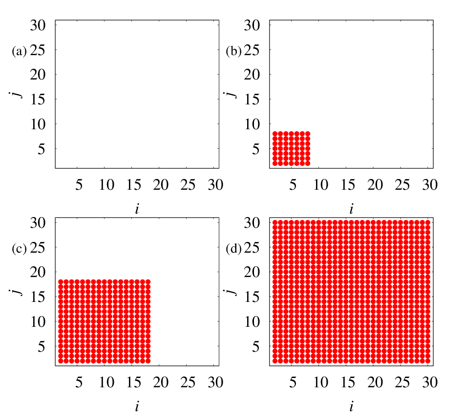
Sequential synchronization can also be visualized using snap shots of the oscillators in the node vs node plots. We regard the oscillators in the array as synchronized when the probability of synchronization , which are indicated by filled circles. Figure 2 shows node vs node diagrams for various values of the coupling strength. For none of the oscillators are synchronized with the drive system (see Fig. 2(a)). Figure 2(b) indicates that the first seven oscillators are synchronized with the drive for . Further increase in the coupling strength results in increase in the size of the synchronized cluster resulting in the formation of sequential synchronization. Figures 2(c) and 2(d) are depicted for and , respectively, illustrating sequential synchronization.
To discuss the nature of the synchronization transition locally, we have calculated the probability of synchronization for some selected systems ( and ) in the array as a function of (see Fig. 3). of the system is plotted as a function of (represented by the filled squares). In the range of , there is an absence of any entrainment between the systems resulting in an asynchronous behavior and is practically zero in this region. However, starting from the value and above, there appear some finite values less than unity attributing to the transition regime. Beyond , attains unit value indicating CS. We have also plotted the probability of synchronization in Fig. 3 for two more selected systems and represented by the asterisk symbol and filled triangles, respectively, indicating the immediate transition to CS locally. The system attains CS at and the system reaches the CS state at . From this figure, one can understand the occurrence of sequential synchronization of the individual systems (locally) in the array as a function of the coupling strength. To explain global (macroscopic) synchronization phenomenon, we have calculated the average probability of synchronization () of the systems as a function of and depicted it in Fig. 3 (represented by the filled circles). It confirms sequential synchronization by gradual increase in as a function of (which indeed exactly matches with Fig. 1).

Next, in the transition regime, we observe intermittent synchronization in every individual system and this can be characterized qualitatively by a difference in the magnitudes of the states between the systems (,) for selected ones ( and ). Figure 4(a-c) shows intermittent synchronization in the above mentioned systems for and , respectively. We also find that the synchronization quality in the transition region depends on the respective positions of the response systems from the drive, as well as on the distance between the two units in the system and the coupling strength. We have additionally plotted the difference between the systems and for the above set of values of coupling strength (Fig. 4(d-f)) to demonstrate the above features.
The statistical features associated with the intermittent dynamics is also analyzed by the distribution of the laminar phases with amplitudes less than a threshold value of (here we have choosen and ). A universal asymptotic power law distribution is observed for the above threshold value of with the exponent . Fig. 5 shows the laminar phase distribution of the above selected systems. The filled circles represent a laminar distribution of the system for , the filled triangles correspond to the laminar distribution of the system for and the filled squares represent a laminar distribution of the system for which clearly display the power law scaling, a typical characterization of on-off intermittency. It should be noted that this result does not change for a large range of .
To understand the phenomenon of intermittent synchronization transition globally in the whole array, we have calculated the average difference () of the () systems in the array with the drive . Figures 6(a) and 6(b) show the average difference for the coupling strengths and , respectively.

The reason behind sequential synchronization transition is in accordance with the sequential stabilization of all the unstable periodic orbits of the response systems in the array as a function of the coupling strength. It is a well established fact that a chaotic/hyperchaotic attractor contains an infinite number of UPOs of all periods. Synchronization between the coupled systems is said to be stable, if all the UPOs of the response systems are stabilized in the transverse direction to the synchronization manifold. Consequently, all the trajectories transverse to the synchronization manifold converge to it for suitable values of . For sequential synchronization, the UPOs in the complex synchronization manifold of the response systems near to the drive are stabilized first for appropriate threshold values of the coupling strength as it is increased, while the UPOs of the far away systems remain unstable for these values of . Once the coupling is increased further, the UPOs of the far away systems are gradually stabilized as a function of the coupling strength. Unfortunately, methods for locating UPOs have not been well established for time-delay systems, which has hampered a qualitative proof for the gradual stabilization of UPOs by locating them.
III Synchronization in a piecewise linear time-delay systems: Linear array with bidirectional coupling
In this section, we consider an array of mutually coupled (bidirectional coupling) piecewise linear time-delay systems with identical subunits. The dynamical equation then becomes
| (7) |
where . We choose open end boundary conditions. The parameter values are the same as in Sec. II. The nonlinear function is chosen as in Eqs. (2)-(II). In the mutual coupling case there are no drive and/or response systems where each and every oscillator shares the signals mutually with its two nearest neighbors. So the synchronization transition is instantaneous due to the mutual sharing of the signals and one needs a very large value of to attain CS. In the transition regime, we have observed an intermittent synchronization transition in all the systems simultaneously in the array.

We have calculated the probability of synchronization of all the systems in the array as a function of the coupling strength and the system index (see Fig. 7). In this figure the black color represents the desynchronized state () and CS is represented by the yellow color (light gray) (). The transition regime is indicated by intermediate colors. From this figure one can clearly see that locally every individual system requires large values of to attain CS and globally all the systems synchronize immediately for the same value of .
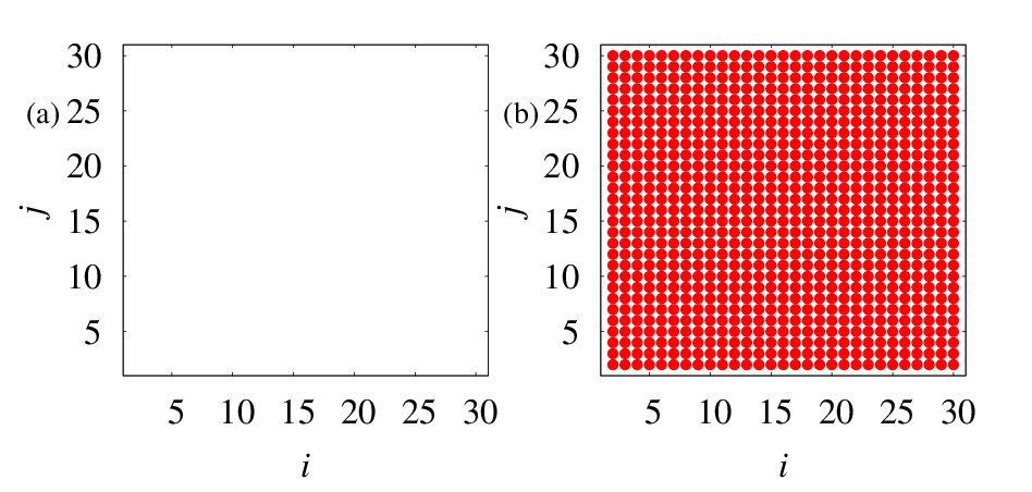
In the mutually coupled array, all the systems get synchronized immediately in a narrow range of the coupling strength, in contrast to sequential synchronization. Figure 8(a) is plotted for , where none of the oscillators in the array are synchronized, whereas for , all the systems are completely synchronized as depicted in Fig. 8(b).

To characterize the nature of synchronization transitions to CS both locally and globally, we again use the probability of synchronization and the average probability of synchronization , respectively. In Fig. 9, we have plotted for some selected piecewise linear systems () as a function of . For instance, we have illustrated for the system in Fig. 9 (represented by the filled squares). From this figure, one can observe that in the range of there is an absence of any entertainment between the systems resulting in asynchronous behavior and is low (). However, for there appear oscillations in in the range of exhibiting intermittent transition. Beyond , indicating perfect CS of the system . We have also calculated for the systems and , represented by asterisk symbols and filled triangles, respectively, which show similar transitions to CS almost at the same value of . We have also confirmed a similar immediate transition to CS in all the systems in the array (see Fig. 7).

To examplify the global synchronization phenomenon, we have calculated the average probability of synchronization () of systems as a function of the coupling strength as shown in Fig. 9 by the filled circles. In the range of ), there is an absence of any synchronization and so is having zero or low values (). In the range of ), is characterized by some finite values less than unity and beyond there is a sudden jump to the value of corrobrating all the systems synchronize immediately at the same value of the coupling strength attributing to the occurrence of global CS. Further, in the transition region we have found long time intervals of high quality synchronization which is interrupted at irregular time intervals by intermittent chaotic bursts simultaneously in all the systems in the array which we call as GIS.
To demonstrate the existence of GIS, we have calculated the spatiotemporal difference () of the array as a function of time and the oscillator index as in Fig. 10 for different values of . Here the black color indicates zero difference () and the red and green colors (dark and light gray) indicate bursting amplitudes. In the absence of coupling (), the systems are evolving independently and so there is no correlation between the systems as shown in Fig. 10(a). If we increase the coupling, we observe several intermittent bursts along with the synchronization as depicted in Figs. 10(b) and 10(c) for and , respectively. From these figures, one can clearly see the occurrence of aperiodic intermittent chaotic bursts along with the synchronized regions simultaneously in all the systems in the array. Beyond one can observe CS as illustrated in Fig. 10(d) where the spatiotemporal difference of the systems is exactly zero for .
To elaborate the occurrence of GIS in the array more clearly, we have calculated the difference between the systems coupled in the array and plotted for some selected systems ( and ) for different values of the coupling strength. The difference between the systems and , , is plotted for and in Figs. 11(a) - 11(c), respectively, which clearly displays the existence of aperiodic intermittent bursts along with the synchronized regions. We have also plotted the difference for the same values of as shown in Figs. 11(e) - 11(g). It is to be noted that in both systems () the intermittent bursts simultaneously occur at the same time and this occurs in all the other systems connected in the array confirming the existence of GIS. In Figs. 11(d) and 11(h) the difference between the systems completely vanish for indicating the occurrence of CS. We have plotted the above figures with time units after leaving a sufficient number of transients.
Further statistical features associated with the intermittent dynamics of the entire array are also analyzed by calculating the distribution of the laminar phases , which is shown in Figs. 12(a) and 12(b) for selected systems and , respectively, for and which clearly display the power law scaling to confirm the on-off intermittency.

The reason for the occurrence of GIS can be explained as follows: As we have already explained, a chaotic attractor can be considered as a pool of infinitely many UPOs of all periods. Synchronization between the systems are asymptotically stable, if all the UPOs of the systems are stabilized in the transverse direction to the synchronization manifold. Consequently, all the trajectories transverse to the synchronization manifold converge to it for suitable values of the coupling strength and this is reflected in the stabilization of the UPOs upon synchronization. From our results, we find that the UPOs of the systems are stabilized in the complex synchronization manifold only for a very large value of coupling strength after a certain threshold value. It is also to be noted that the intermittency transition in the case of a bidirectional coupling configuration is due to the fact that the strength of the coupling contributes only less significantly to stabilize the UPOs as the error in the coupling term in Eq. (7) gradually becomes smaller from the transition regime after a certain threshold value of the coupling strength.
IV Conclusion
In conclusion, we have shown the existence of sequential and instantaneous synchronization transitions in an array of time-delay systems with different coupling configurations. If the systems are coupled with unidirectional configuration, we have observed an immediate synchronization transition to CS microscopically and if we consider the macroscopic synchronization behavior of the entire array we find that the transition region is gradually increasing as a function of due to sequential synchronization which is verified by the probability of synchronization and average probability of synchronization. In the transition regime we have observed the existence of intermittent synchronization. On the other hand, if we consider an array of mutually coupled time-delay systems, every individual system (microscopically) synchronizes immediately for a very large value of and globally (macroscopically) the synchronization transition occurs immediately in the whole array. In the transition region a new type of synchronization called GIS occurs which is characterized by long intervals of high quality synchronization interrupted at irregular times by intermittent chaotic bursts simultaneously in all the systems.
The reason (mechanism) for these two distinct transition scenarios is explained based on unstable periodic orbit theory. The GIS is confirmed using the spatiotemporal difference and a power law behavior of the laminar length distributions with power law scaling. The above studies have been carried out in a well known piecewise linear time-delay system. We have also confirmed the occurrence of the above results for another well known time-delay systems namely the Mackey-Glass system [38] with an array length of and we do observe the same kind of sequential and instantaneous synchronization transitions preceded by GIS for unidirectional and bidirectional coupling configurations, respectively.
Acknowledgements.
The work of R. S. and M. L. is supported by a Department of Science and Technology (DST), IRHPA research project. M. L. is also supported by a Department of Atomic Energy Raja Ramanna fellowship and a DST Ramanna program. D. V. S. and J. K. acknowledge the support from EU under project No. 240763 PHOCUS(FP7-ICT-2009-C) and J. K. acknowledges the support from IRTG 1740(DFG).References
- [1] A. S. Pikovsky, M. G. Rosenblum, and J. Kurths, Synchronization - A Unified Approach to Nonlinear Science (Cambridge University Press, Cambridge, 2001).
- [2] S. Boccaletti, J. Kurths, G. Osipov, D. L. Valladares, and C. S. Zhou, Phys. Rep. 366, 1 (2002).
- [3] J. F. Heagy, N. Platt, and S. M. Hammel, Phys. Rev. E. 49, 1140 (1994).
- [4] P. Ashwin, J. Buescu, and I. Stewart, Phys. Lett. A 193, 126 (1994), Nonlinearity 9, 703 (1994); S. Rim, I. Kim, P. Kang, Y. J. Park, and C. M. Kim, Phys. Rev. E 66, 015205(R) (2002); S. Boccaletti et al,, Phys. Rep. 366, 1 (2002); D. V. Senthilkumar, and M. Lakshmanan, Phys. Rev. E 71, 016211 (2005); M. G. Rosenblum, A. S. Pikovsky, and J. Kurths, Phys. Rev. Lett. 78, 4193 (1997).
- [5] S. C. Venkataramani, B. R. Hunt, and E. Ott, Phys. Rev. E 54, 1346 (1996).
- [6] T. Kanamaru, Int. J. Bifurcation and Chaos 16, 3309 (2006).
- [7] J. L. Perez Velazquez et. al, Eur. J. Neurosci. 11, 2571 (1999).
- [8] A. Hramov et. al, Chaos 16, 043111 (2006).
- [9] M. Sauer, and F. Kaiser, Phys. Lett. A 243, 38 (1998).
- [10] V. Flunkert, O. DHuys, J. Danckaert, I. Fischer, and E. Schll, Phys. Rev. E. 79, 065201(R) (2009).
- [11] D. J. Gauthier, and J. C. Bienfang, Phys. Rev. Lett. 77, 1751 (1996).
- [12] Y. H. Yu, K. Kwak, and T. K. Lim, Phys. Lett. A 198, 34 (1995).
- [13] R. L. Viana, C. Grebogi, S. E. de S Pinto, S. R. Lopes, A. M. Batista, and J. Kurths, Physica D 206, 94 (2005).
- [14] H. L. Yang, and E. J. Ding, Phys. Rev. E 54, 1361 (1996).
- [15] M. Bottiglieri, and C. Godano, Phys. Rev. E 75, 026101 (2007).
- [16] J. H. E. Cartwright, M. O. Magnasco, O. Piro, and I. Tuval, Phys. Rev. E 68, 016217 (2003).
- [17] C. Huepe, and M. Aldana, Phys. Rev. Lett. 92, 168701 (2004).
- [18] X. Wang, S. Guan, Y-C. Lai, B. Li, and C. H. Lai, Europhys. Lett. 88, 28001 (2009).
- [19] L. Zhao, Y. C. Lai, and C. W. Shih, Phys. Rev. E. 72, 036212 (2005).
- [20] S. Boccaletti, D. L. Valladares, Phys. Rev. E 62, 7497 (2000).
- [21] A. Pikovsky, G. Osipov, M. Rosenblum, M. Zaks, and J. Kurths, Phys. Rev. Lett. 79, 47 (1997).
- [22] K. J. Lee, Y. Kwak, and T. K. Lim, Phys. Rev. Lett. 81, 321 (1998).
- [23] A. E. Hramov, A. A. Koronovskii, Europhys. Lett. 70, 169 (2005).
- [24] D. V. Senthilkumar, and M. Lakshmanan, Phys. Rev. E 76, 066210 (2007).
- [25] M. Lakshmanan, and D. V. Senthilkumar, Dynamics of Nonlinear Time-Delay Systems (Springer-Verlag, Berlin, 2011).
- [26] R. Suresh, D. V. Senthilkumar, M. Lakshmanan, and J. Kurths, Phys. Rev. E 82, 016215 (2010).
- [27] X. Wu, J. Zhang, and Z. Zhao, Adaptive Synchronization of Chaotic Neural Networks with Time Delay ((IEEE, 2010), pp. 5125-5130.
- [28] LiuYaowen, GeGuangming, ZhaoHong, WangYinghai, and GaoLiang, Phys. Rev. E 62, 7898 (2000).
- [29] G. D. VanWiggeren, R. Roy, Science 279, 1198 (1998).
- [30] A. Argyris et. al,, Nature (London) 438, 343 (2005).
- [31] S. Banerjee, D. Ghosh, A. Ray, and R. R. Chowdhury, Europhys. Lett. 81, 20006 (2008).
- [32] J. Liang, Z. Wang, Y. Liu, and X. Liu, IEEE Trans Neural Networks 19, 1910 (2008).
- [33] D. V. Senthilkumar, K. Srinivasan, K. Murali, M. Lakshmanan, and J. Kurths, Phys. Rev. E. 82, 065201(R) (2010).
- [34] K. Srinivasan, D. V. Senthilkumar, K. Murali, M. Lakshmanan, and J. Kurths, Chaos 21, 023119 (2011).
- [35] M. N. Lorenzo, I. P. Mario, V. Perez-Muuzuri, M. A. Matías, and V. Perez-Villar, Phys. Rev. E 54, R3094 (1996).
- [36] M. A. Matías, and J. Gémez, Phys. Rev. Lett. 81, 4124 (1998).
- [37] C. Kirst, T. Geisel, and M. Timme, Phys. Rev. Lett. 102, 068101 (2009).
- [38] M. C. Mackey, and L. Glass, Science 197, 287 (1977).