Pseudogap Effects of Fermi Gases in the Presence of A Strong Effective Magnetic Field

The role of non-condensed pairs in fermionic and bosonic superfluids under the influence of a strong effective magnetic field has not been clearly addressed in the literature. One could imagine that in anticipation of the vortex configuration of the superfluid phase, these non-condensed pairs exhibit some degree of inhomogeneity. The goal of the present paper is to investigate this normal phase. Our study should lead to a reconsideration of previous work on rotating cold Fermi gases [1, *Radzihovskyrotation, *Cooperrotation] where the upper critical rotation frequency was computed under the assumption that non-condensed pairs were not present, even in the BEC regime. It may also be relevant to “normal state vortex” models [4, 5] which are argued to be important in high temperature superconductivity. Furthermore, we note the community excitement over proposals to establish strong effective magnetic fields through “artificial” means. These are implemented through either asymmetric tunneling in a lattice [6] or geometric gauge potentials [7, 8]. This makes our work on the interplay of rapid rotation and superfluidity particularly topical.

Finally, we believe our work bears on a puzzling aspect of superconductivity in high magnetic fields, even within the BCS framework. As has been emphasized in the literature, the degeneracy of Landau levels implies that the fluctuations around the BCS phase are effectively one-dimensional [9], representing the free propagation of particles along the field direction; this is well known [10, *ullah_1991] to be problematic for stable superconductivity.

In this paper we suggest that the origin of this latter difficulty is due to the fact that in BCS theory, Cooper pairs only exist in a condensed state. Here we show that by introducing non-condensed pairs associated with a finite pairing gap (or “pseudogap”) at the onset of condensation, a strict “dimensional reduction”[9] is no longer present; three-dimensional behavior leading to stable condensation at $T_{c}$ can then occur. Our approach is to be contrasted with previous attempts [12, *alexandrov_1993] to address the early concerns raised by Schafroth [10] in Bose gases. Here we emphasize the contrast with BCS theory, where the only pairs under consideration are in the condensate.

One goal of this paper is to stimulate experimental searches for the predicted precursors of the vortex configurations below $T_{c}$. Here we characterize the degrees of freedom associated with non-condensed pairs and demonstrate that they create pair density inhomogeneities. Although these excited pairs become progressively more important as the superconductor crosses from BCS to BEC (and pairing becomes more stable), they may well be necessary even in the BCS limit for stable condensation. These ideas relate to earlier work on pair density waves [14], but are in contrast to previous studies on the interplay of a pseudogap and magnetic field [15, *pieri_2002] where density inhomogeneities were not contemplated.

To understand these non-condensed pairs we are guided by Landau-Ginzburg (LG) theory where in zero magnetic field non-condensed pairs are associated with finite center of mass momentum $\boldsymbol{q}$; these represent gapless excitations as $\boldsymbol{q}\rightarrow 0$. In non-zero field, the natural counterpart should be associated with slightly distorted configurations of the vortices. These pair excitations become gapless as they approach the lowest energy superconducting vortex configuration. However, we also emphasize that these non-condensed pairs are distinct from previously considered Landau-Ginzburg vortex lattice fluctuations which only address the condensate [17, 18]. We now proceed to describe how we incorporate these non-condensed pairs, and their effects at and above the superfluid transition.

Rewriting the Gor’kov Equations We begin with a BCS-type theory, and proceed to separate out the effects of pairing and condensation by introducing non-condensed pairs appropriate for high effective magnetic fields. First, we introduce a Landau level representation for the Gor’kov equations. The real-space Gor’kov coupled equations for the gap $\Delta(\boldsymbol{r})$ and the fermionic Green’s function $G(\boldsymbol{r},\boldsymbol{r}^{\prime};i\omega)$ are:

Throughout this paper $i\omega$ ($i\Omega$) will be used to denote discrete fermionic (bosonic) Matsubara frequencies, with the traditional subscripts omitted for clarity. Introducing a Landau level basis for the fermions indexed by $m=(N,p,k_{z})$ where $N$ is the Landau level, $p$ the degenerate Landau level index, and $k_{z}$ the momentum parallel to the magnetic field, we write the bare Green’s function $G^{0}(\boldsymbol{r},\boldsymbol{r}^{\prime};i\omega)=\sum_{n}\psi_{n}(\boldsymbol{r})\psi_{n}^{\dagger}(\boldsymbol{r}^{\prime})/(i\omega-\xi_{n})$ where $\xi_{n}$ is the single-particle energy; the dressed Green’s function is $G(\boldsymbol{r},\boldsymbol{r}^{\prime};i\omega)=\sum_{mm^{\prime}}G_{mm^{\prime}}(i\omega)\psi_{m}(\boldsymbol{r})\psi^{\dagger}_{m^{\prime}}(\boldsymbol{r}^{\prime})$ [19]. The self energy, given by $\Sigma(\boldsymbol{r},\boldsymbol{r}^{\prime};i\omega)=-\Delta(\boldsymbol{r})\Delta^{\dagger}(\boldsymbol{r}^{\prime})G_{0}(\boldsymbol{r}^{\prime},\boldsymbol{r};-i\omega),$ is rewritten as $\Sigma_{mm^{\prime}}(i\omega)=-\sum_{n}G^{0}_{n}(-i\omega)\Delta_{mn}\Delta^{\dagger}_{m^{\prime}n},$ and the number equation necessary for a self-consistent solution is $N=\frac{2}{\beta}\sum_{m,i\omega}G_{mm}(i\omega)$. Defining $\Delta_{mn}\equiv\int d\boldsymbol{r}\Delta(\boldsymbol{r})\psi_{m}^{\dagger}(\boldsymbol{r})\psi_{n}^{\dagger}(\boldsymbol{r})$, and integrating over position variables yields

These correspond to Eqs. (1)-(2) respectively in the Landau level basis. Eq. (4) is equivalent to that found elsewhere in Refs. [20, 21]. As in these references we restrict our consideration to intra-Landau level pairing. This assumption is important for arriving at a tractable scheme and a good approximation in the high-field regime [22].

It is useful to recognize that the nonlinear gap equation, Eq. (4), applies to all $T\leq T_{c}$. This nonlinearity is reflected in the presence of one dressed and one bare Green’s function, as opposed to the two bare Green’s functions associated with the instability onset in strict BCS theory. This gap equation can be thought of as a Bose-Einstein condensation condition [23] which reflects the vanishing chemical potential of the pairs below $T_{c}$, and which becomes finite above.

Characterizing Non-condensed Pairs Outside of the weak-coupling limit, pairs may form in kinetically excited states [23]. These pairs appear above the superfluid transition temperature $T_{c}$, corresponding to a pseudogap phase, and should also persist below the transition. To include these non-condensed pairs, we must therefore introduce variables corresponding to their excitation parameters.

In the $z$-direction parallel to the field, we introduce a total momentum $q_{z}=k_{z_{1}}+k_{z_{2}}$ of the pair, in analogy with the zero-field case [23]. Perpendicular to the effective magnetic field, however, both condensed and non-condensed pairs may lie in the same Landau level. We posit, therefore, that non-condensed pairs correspond to different real-space gap configurations $\Delta(\boldsymbol{r})$, which we now parametrize by $\zeta$. We single out $\zeta_{0}$ which denotes the condensate gap configuration. In general non-condensed pairs can occupy other functional forms of $\Delta(\boldsymbol{r})$, for which the parameter $\zeta$ will generally be close to $\zeta_{0}$, associated with low-energy excitations as described below.

In our mean-field approach, we consider the condensate function $\Delta(\boldsymbol{r},\zeta_{0})$ to be that of the optimal triangular lattice. Non-condensed pairs can then occupy a two-dimensional continuum of other Abrikosov lattice configurations. Mathematically, we use the Landau gauge $\boldsymbol{A}=(0,H\hat{\boldsymbol{x}},0)$ and an Abrikosov lattice with unit vectors $\boldsymbol{a}=(0,a,0)$ and $\boldsymbol{b}=(b_{x},b_{y},0)$, where $ab_{x}=\pi l_{H}^{2}$ with $l_{H}=\sqrt{\hbar c/eH}$ the magnetic Hall length. The two clear mean-field distortions available to excited pairs are associated with changing $b_{x}/a$, and changing $b_{y}/a$ (see Fig. 1) [24]. Both of these are higher in energy relative to the optimal Abrikosov lattice. We then follow Ref. [24] in setting $\zeta=b_{y}/a+ib_{x}/a$, for which the optimal triangular lattice condensate configuration is $\zeta_{0}=1/2+i\sqrt{3}/2$. To transform to state-space, we can associate with each distortion a normalized real-space gap configuration $\Delta^{0}(\boldsymbol{r},\zeta)$, where $\int d\boldsymbol{r}\left|\Delta^{0}(\boldsymbol{r},\zeta)\right|^{2}=1$, from which $\Delta^{0}_{mn}(\zeta)\equiv\int d\boldsymbol{r}\Delta^{0}(\boldsymbol{r},\zeta)\psi_{m}^{\dagger}(\boldsymbol{r})\psi_{n}^{\dagger}(\boldsymbol{r})$ can also be calculated.

In summary, these non-condensed pairs are now specified by three degrees of freedom, thereby compensating the problematic dimensional reduction and restoring the possibility of stable condensation. We can also use these parameters to rewrite the gap equation, Eq. (4), by defining a pair susceptibility $\chi(\zeta,q_{z};i\Omega)\equiv$

so that Eq. (4) assumes a simple and suggestive form

In Eq. (5), $G^{0}$ is written in terms of the Landau level $N$ and $z$-momentum of $m=(N,p,k_{z})$ (with $N_{m}=N_{m^{\prime}}$ and $k_{z_{m}}=k_{z_{m^{\prime}}}$) and $\phi^{2}_{mm^{\prime}}(\zeta)=\sum_{n}\Delta^{0}_{mn}(\zeta)\Delta^{0{\dagger}}_{nm^{\prime}}(\zeta).$

Green’s Function of Non-condensed Pairs

Equation (6) suggests that there is a $t$-matrix (or a summation of particle-particle ladder diagrams), which is related to the pair susceptibility Eq. (5) and which diverges at and below $T_{c}$. More precisely, we have shown in Ref. [25] that, not surprisingly, this $t$-matrix is given by

Moreover, this $t$-matrix will lead to a self energy contribution [25] in parallel with what is found in Gor’kov theory via the condensate t-matrix, $\Sigma^{\mathrm{pg}}_{mm^{\prime}}(i\omega)=$

This self energy is then fed back into the Green’s function which enters into the pair susceptibility, and into the self-consistently determined $t$-matrix.

Because of the mixing through the self-energy of an infinite number of real-space gap configurations, the calculation of the pair susceptibility $\chi$ is not analytically tractable. To make progress without the distraction of heavy numerics, we approximate the pair susceptibility as $\chi(\zeta,q_{z};i\Omega)\approx$

where we have, in effect, decomposed $G_{mm^{\prime}}$ into separate contributions each associated with a distinct lattice structure. In this way Eq. (8), which becomes

determines the Green’s functions $G_{mm^{\prime}}(\zeta;i\omega)$.

Importantly, we can further write that $\Sigma_{mm^{\prime}}^{\mathrm{pg}}(\zeta;i\omega)\approx-\phi^{2}_{mm^{\prime}}(\zeta)\left|\Delta^{\mathrm{pg}}\right|^{2}G^{0}_{N}(-k_{z};-i\omega),$ where the gap contribution from the non-condensed pairs is given by $\left|\Delta^{\mathrm{pg}}\right|^{2}\equiv-\frac{1}{\beta}\sum_{\zeta,q_{z},i\Omega}t(\zeta,q_{z};i\Omega).$ To derive this simplified (BCS-like) expression for the pseudogap self energy in a strong “magnetic field” we have used the fact that the small chemical potential of the pairs implies that $t^{\mathrm{pg}}$ is strongly peaked around $(q_{z},i\Omega)=(0,0)$ near and below $T_{c}$. When we consider a diagonal pairing scheme [21], the Green’s function that results has a familiar BCS form $G_{mm}(\zeta,i\omega)=(i\omega+\xi)/\left[(i\omega)^{2}-\xi^{2}-\left|\Delta^{\mathrm{pg}}\right|^{2}\phi_{mm}^{2}(\zeta)\right]$.

In effect, the main approximation we have made is to consider each vortex configuration as an “independent system,” sharing self-consistently the same magnitude of the energy gap $\left|\Delta^{\mathrm{pg}}\right|^{2}$, but possessing a distinct real-space gap parameter $\Delta^{0}(\boldsymbol{r},\zeta)$ which in turn provides a unique form factor $\phi^{2}_{mm^{\prime}}(\zeta)$ in the self-energy. This is similar in approach to considering an LG energy functional for the different forms of the gap parameter. In contrast to LG theory, here we explicitly incorporate the fermionic nature of the pairing.

Fermionic Constituents of the Pairs This discussion has been cast in terms of the basis eigenstates $\psi_{m}(\boldsymbol{r})$ which we now need to specify. Here we use the magnetic translation group basis [26, 21, 27, *norman_1995, *nicopoulos_1991], although we have also explored an alternative orbit-center based pairing basis [20, 25]. Magnetic translation group (MTG) pairing relates to the Abrikosov lattice and is associated with a Bloch-like index $\boldsymbol{k}=(k_{x},k_{y})$. The unit cell for the MTG has unit vectors $2\boldsymbol{a}$ and $\boldsymbol{b}$, which means in turn that the state basis is dependent on $\zeta$. Pairing for the $\zeta$ appropriate to the basis occurs with a single partner between opposite $\boldsymbol{k}$ [21], i.e. $\Psi^{\mathrm{pair}}_{N,\boldsymbol{k},q_{z}}(\boldsymbol{r})=\psi^{\mathrm{fermion}}_{N,\boldsymbol{k},k_{z},\uparrow}(\boldsymbol{r})\psi^{\mathrm{fermion}}_{N,-\boldsymbol{k},-k_{z}+q_{z},\downarrow}(\boldsymbol{r})$. $\Delta^{0}_{mn}(\zeta)$ for these pairs is computed elsewhere [21, 25].

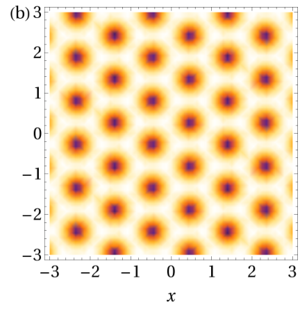
Results With this formalism in place, we are in a position to examine the underlying physics of how superfluidity with pre-formed pairs takes place in the presence of a high effective magnetic field. This addresses the difficulty that a stable transition seems to require some inhomogeneity in the normal state [10, *ullah_1991]. In Fig. 2 we plot the $t$-matrix vs. lattice configuration $\zeta$ for three different sets of effective temperatures, demonstrating that as condensation is approached from higher temperatures, the occupation of lattice states near the ideal triangular Abrikosov lattice ($\zeta=\zeta_{0}$) begins to peak. Precisely at $T=T_{c}$, a delta function results at $\zeta=\zeta_{0}$. Nevertheless at the transition there is still considerable weight associated with other lattice configurations reflecting the fact that the pseudogap $\left|\Delta^{\mathrm{pg}}\right|^{2}$ remains finite. The condensate contribution corresponds to a perfect triangular lattice which necessarily has small weight near $T_{c}$.

Of particular interest is the real space reflection of these distorted Abrikosov lattice contributions. To illustrate this precursor vortex configuration we evaluate

which is a weighted average of the gap (squared). This is compared with the counterpart for a fully condensed system in Fig. 3. By addressing the square of the gap, we emphasize that there is no phase information in the normal state pseudogap. It should be noted that the point $\boldsymbol{r}=0$ is chosen as a point of “symmetry breaking” or pinning center which breaks the translational symmetry available in the selection of each $\Delta^{0}(\boldsymbol{r},\zeta)$.

Conclusions In this paper we have addressed an important and in principle testable prediction in the cold Fermi gases: the presence of precursor vortex configurations in the normal (pseudogap) phase. Indeed, the role of non-condensed bosons in rapidly rotating condensates has not been elucidated even for the atomic Bose gases. Here, too, one might expect a precursor vortex configuration. We have, moreover, elucidated the nature and role of excited pair states throughout the BCS-BEC crossover in high effective magnetic fields, showing that these are associated with distortions of the Abrikosov lattice.

The concept of a “normal state vortex” liquid is also rather widely discussed in the context of high $T_{c}$ superconductors [4, 5]. There are, of course, a host of controversial issues associated with the cuprate pseudogap, but Fig. 3 illustrates one scenario for how one might think about this phenomenon in the context of pre-formed pairs in a strong magnetic field.

The experimental implementation of this work in cold gases will depend on reaching a regime in which the Landau level spacing is much larger than the gap, although we expect the qualitative aspects regarding the role of pair density inhomogeneities to apply to much lower fields. While rapid rotation may be able to reach this regime, current proposals for artificial fields [6, 7, 8] also show promise. In this paper, two spin states which interact via a Feshbach resonance must both feel the same effective field, which may make geometric gauge-based proposals more challenging. Regardless of the implementation, reaching this regime would facilitate a large body of new research into BCS-BEC phenomena.

We are grateful to Jonathan Simon for helpful discussions. This work is supported by NSF-MRSEC Grant 0820054. P.S. acknowledges support from the Hertz Foundation.

References

- [1] H. Zhai and T.-L. Ho, Phys. Rev. Lett. 97, 180414 (2006).
- [2] M. Y. Veillette, D. E. Sheehy, L. Radzihovsky, and V. Gurarie, Phys. Rev. Lett. 97, 250401 (2006).
- [3] G. Moller and N. R. Cooper, Phys. Rev. Lett. 99, 190409 (2007).
- [4] L. Li, Y. Wang, S. Komiya, S. Ono, Y. Ando, G. D. Gu, and N. P. Ong, Phys. Rev. B 81, 054510 (2010).
- [5] P. W. Anderson, Nat. Phys. 3, 160 (2007).
- [6] A. R. Kolovsky, Europhys. Lett. 93, 20003 (2011).
- [7] J. Dalibard, F. Gerbier, G. Juzeliunas, and P. Öhberg, Rev. Mod. Phys. 83, 1523 (2011).
- [8] N. R. Cooper, Phys. Rev. Lett. 106, 175301 (2011).
- [9] P. A. Lee and S. R. Shenoy, Phys. Rev. Lett. 28, 1025 (1972).
- [10] M. R. Schafroth, Phys. Rev. 100, 463 (1955).
- [11] S. Ullah and A. T. Dorsey, Phys. Rev. B 44, 262 (1991).
- [12] A. Alexandrov, D. Samarchenko, and S. Traven, Sov. Phys. JETP 66, 567 (1987).
- [13] A. S. Alexandrov, Phys. Rev. B 48, 10571 (1993).
- [14] Z. Tesanovic, Physica C 220, 303 (1994).
- [15] Y. J. Kao, A. P. Iyengar, Q. Chen, and K. Levin, Phys. Rev. B 64, 140505 (2001).
- [16] P. Pieri, G. C. Strinati, and D. Moroni, Phys. Rev. Lett. 89, 127003 (2002).
- [17] T. Maniv, V. Zhuravlev, I. Vagner, and P. Wyder, Rev. Mod. Phys. 73, 867 (2001).
- [18] B. Rosenstein and D. Li, Rev. Mod. Phys. 82, 109 (2010).
- [19] M. G. Vavilov and V. P. Mineev, J. Exp. Theor. Phys. 85, 1024 (1997).
- [20] J. C. Ryan and A. K. Rajagopal, Phys. Rev. B 47, 8843 (1993).
- [21] S. Dukan and Z. Tesanovic, Phys. Rev. B 49, 13017 (1994).
- [22] Z. Tesanovic and P. D. Sacramento, Phys. Rev. Lett. 80, 1521 (1998).
- [23] Q. Chen, J. Stajic, S. Tan, and K. Levin, Physics Reports 412, 1 (2005).
- [24] D. Saint-James, G. Sarma, and E. J. Thomas, Type II superconductivity (Pergamon Press, Oxford, 1969).
- [25] P. Scherpelz, D. Wulin, B. Šopík, K. Levin, and A. K. Rajagopal, arXiv:1112.1112v3 (2012).
- [26] S. Dukan, A. V. Andreev, and Z. Tesanovic, Physica C 183, 355 (1991).
- [27] H. Akera, A. H. MacDonald, S. M. Girvin, and M. R. Norman, Phys. Rev. Lett. 67, 2375 (1991).
- [28] M. R. Norman, A. H. MacDonald, and H. Akera, Phys. Rev. B 51, 5927 (1995).
- [29] V. N. Nicopoulos and P. Kumar, Phys. Rev. B 44, 12080 (1991).