HU-EP-12/23
Three-Point Functions of Twist-Two Operators
in SYM at One Loop
Jan Plefkaa, Konstantin Wiegandta,b
a Institut für Physik, Humboldt-Universität zu Berlin,
Newtonstraße 15, 12489 Berlin
b II. Institut für Theoretische Physik, Universität Hamburg,
Luruper Chaussee 149, 22716 Hamburg
Abstract
We calculate three-point functions of two protected operators and one twist-two operator with arbitrary even spin in theory to one-loop order. In order to carry out the calculations we project the indices of the spin operator to the light-cone and evaluate the correlator in a soft-limit where the momentum coming in at the spin operator becomes zero. This limit largely simplifies the perturbative calculation, since all three-point diagrams effectively reduce to two-point diagrams and the dependence on the one-loop mixing matrix drops out completely. The results of our direct calculation are in agreement with the structure constants obtained by F.A. Dolan and H. Osborn from the operator product expansion of four-point functions of half-BPS operators.
1 Introduction and Conclusions
The full solution of theory is equivalent to the ability of calculating any observable of interest in this quantum field theory exactly or perturbatively to arbitrary order in the coupling constant. In recent years, such impressive achievements have indeed been made for certain observables in planar , largely due to the existence of integrability [1, 2, 3, 4] in the AdS/CFT correspondence [5, 6, 7], see [8] for a review.
Using the methods of integrability, all-order conjectures, e.g. for the cusp anomalous dimension of twist two operators could be obtained [9, 10]. Using this, also for scattering amplitudes of four and five external particles in planar , all-order results became available [11, 12]. These all-order results were achieved using the duality between MHV amplitudes and light-like Wilson loops [13, 14, 15], see [16, 17] for reviews.
Given these results, it is natural to ask, whether similar advances can be made for three-point functions of gauge invariant operators. Not only are three-point functions the next natural correlators to address after two-point functions, but they possess a particular importance due to the operator product expansion (OPE). Given the knowledge of all structure constants that appear in the theory, one can in principle construct any higher-point correlation function using the OPE. Therefore, all-order results for structure constants, together with all-order results for anomalous dimensions yield important information on any higher-point function.
The form of three-point functions is fixed by conformal symmetry and the only dependence on the coupling constant is contained in the anomalous dimensions of the operators and the structure constants which receive radiative corrections in the coupling
| (1) |
Similarly as for two-point functions, there are non-renormalisation theorems for three-point correlators of half-BPS operators, which guarantee that they do not get quantum corrections [18, 19, 20, 21, 22, 23].
Direct computations of three-point functions in theory have been performed in [24, 25, 26, 27, 28, 29, 30, 31, 32]. In [33] a large number of three-point functions involving scalar primary operators of up to and including length five is considered.
The role of integrability for three-point function calculations was first addressed in [28, 27, 29]. Applications of integrability methods can be found in [34, 35, 36, 37] at tree-level and in [38, 37] for loop-level three-point functions of scalar single trace operators. It does indeed turn out, that three-point functions can be studied efficiently using integrability.
The question of a weak-strong coupling matching was addressed in [35, 39, 40, 41, 42, 43]. The SL(2) sector was adressed in [43] and agreement between the structure constants at weak and strong coupling was found, where a BPS state and two operators with large spin were considered at tree-level. It would be interesting to promote this study to the loop-level, which requires the knowledge of the correlator of one BPS operator and two operators with spin at one-loop level. Furthermore, it would be interesting to see, how one can make use of integrability methods in order to calculate this correlator at loop-level.
Here, we make a first step towards this direction by providing a direct field theory computation of three-point correlators with two protected operators and one twist-two operator. This calculation serves as a starting point for the case of two operators with spin, where several distinct space-time structures enter with a priori different structure constants, see e.g. [44], [45]. A direct calculation is possibly more suitable for the development of integrability methods than the extraction of the same coefficient from the OPE.
More explicitly, here we calculate three-point functions in theory involving two protected scalar operators
| (2) |
and one twist-two operator with arbitrary even spin , which is totally symmetric and traceless in all indices and schematically of the form
| (3) |
where the ellipses stand for a certain distribution of the derivatives, which is given explicitly in section 2. Conformal symmetry fixes the three-point functions up to the structure constants . We use the light-cone projection, see appendix A.2, where all indices are contracted with a light-like vector . Then the correlator with the renormalised operator , see (9), reads
| (4) |
where is the twist (dimension minus spin) of the operator ,
| (5) |
and where . Note, that the dimension of the twist operator and the structure constants both acquire corrections in perturbation theory
| (6) |
In order to carry out the calculations we evaluate the correlator in a soft-limit, where the momentum coming in at the spin operator becomes zero. In position space this corresponds to an integration over the corresponding point
| (7) |
This limit largely simplifies the perturbative calculation, since all three-point diagrams effectively reduce to two-point diagrams and the dependence on the one-loop mixing matrix drops out completely, as we will see in section 2. We find that the correction to the structure constant takes the simple form
| (8) |
where are generalised harmonic sums , . The result is in agreement with the extraction of the structure constants from the analysis of the operator product expansion (OPE) of four-point functions of half-BPS operators [46]. Recently, the OPE and the three-loop expression for the four-point correlator of half-BPS operators [47] were used to extract the structure constants up to three loops [48]. Our calculation thus directly confirms the results obtained from the OPE.
In the following sections we will only summarise the main steps of our calculation in order to keep the presentation short, more details will be made available in [49].
2 Three-Point Functions of Twist Operators
We use the mostly minus metric and the conventions as given in Appendix A and adapt the notation from [50]. The renormalised twist-two operators are given by
| (9) |
where the tree-level correlator is
| (10) |
the coefficients are related to the Gegenbauer polynomials as in (37) and the one-loop mixing matrix in the conformal scheme has the form
| (11) |
At one-loop level the divergent part of the renormalisation matrix is diagonal with and determines the anomalous dimension via . The finite matrix diagonalizes the anomalous dimension matrix at higher-loop level and accounts for non-diagonal contributions to the two-point functions at loop-level. We do not specify , since it drops out in the limit that we consider. The operators given by (9) then have diagonal, conformal two-point functions also at loop-level and are fixed up to the normalization
| (12) |
where and . In order to read-off the structure constants in the limit (7) we have to integrate (4) over , which yields
| (13) |
where is a normalisation factor explicitly given in (45). By calculating the left-hand side in the limit one can thus easily read-off the structure constants, after Fourier transforming the momentum space expression11 1 An analogue of this procedure appears in [51], where a deformation of the N = 4 SYM Lagrangian by integrated local operators is considered and two-point functions of the deformed theory are studied at leading order in the deformation parameter.
3 Tree-Level Calculation
In momentum space, the tree-level three-point function with the twist-operator in the representation (38) reads
| (14) |
Now we take the limit in momentum space. Then, due to the factor only the term with the highest power, i.e. , in the Gegenbauer polynomial can survive. The corresponding coefficient reads
| (15) |
Thus, in this limit the three-point integral in (14) becomes a two-point integral with a doubled propagator
| (16) |
which can easily be solved using (42) in the appendix. Fourier transformation to -space using (41) and insertion of the coefficients yields
| (17) |
Comparing with (13) we can directly read off the tree-level structure constant for and arbitrary even spin
| (18) |
4 One-Loop Calculation
In order to read-off the one-loop structure constant we have to compute the renormalised three-point function using the renormalised operator given by (9)-(11). From
it is however immediately clear, that the finite matrix drops out in the limit that we consider, which vastly simplifies the calculation. As can be seen from (11), we then only need to calculate the one-loop diagrams and subtract the tree-level contribution22 2 It needs to be evaluated including terms, because it is multiplied with . multiplied with the renormalisation constant . The one-loop diagrams that enter the calculation are shown in figure 1.
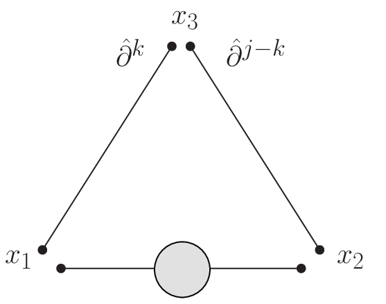
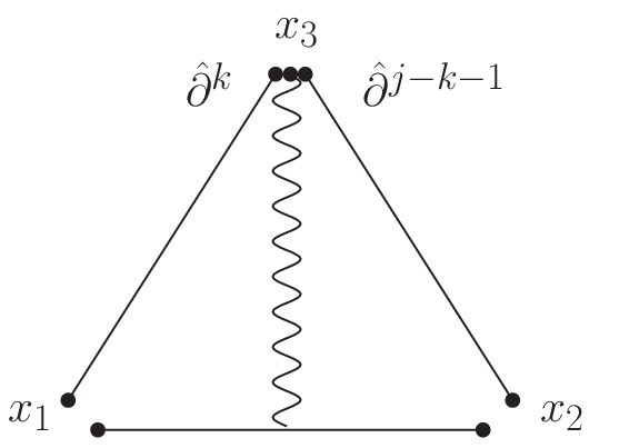


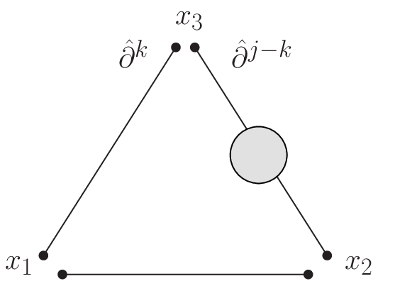

It is instructive to write down all diagrams before employing the limit and to convince oneself that diagrams which could lead to ambiguities, such as the diagram in figure 1g, which vanishes in dimensional regularisation when taking the limit, cancel with contributions from other diagrams.
Indeed, all diagrams with a scalar four-point interaction vertex, i.e. fig. 1c, 1g, 1k cancel against contributions from fig. 1b, 1f, 1j, which becomes clear when considering the decomposition of diagrams with two gluon vertices into scalar integrals, see figure 2.


For , the diagrams in the last column do not appear, since there is no covariant derivative that the gauge field at could arise from and half of the diagrams 1e, 1a cancels against a contribution from 1f, half of the diagrams 1a, 1i cancels against a contribution from 1j and half of the diagrams 1e, 1i cancels against a contribution from 1b. The remaining finite contributions from 1b, 1f, 1j cancel due to a relation between scalar three-point integrals given in [52]. Thus for all contributions exactly cancel, which is due to the fact that in this case all of the operators are protected.
For the above cancellations between divergent diagrams where the divergence is located at the points resp. , i.e. where the BPS operators sit, remain true as one would expect33 3 Would divergences at these points remain, the operators acquired an anomalous dimension, we do however have protected operators with vanishing anomalous dimension at .. The cancellations between half of the diagrams 1e, 1i with a contribution from 1b does however not take place anymore, and the spin- operator at acquires an anomalous dimension . For the remaining diagrams in the limit , for the same reason as in the tree-level calculation, we only need the coefficient with the highest power of the Gegenbauer polynomial that was given in (15). Since and is even we find the same result for all diagrams which are equal under . The integrals turn into simple two-point integrals that can be easily solved using (42). Denoting from now on we find
| (19) | ||||
where is defined in (43). As mentioned before, half of the self-energy diagrams in fig. 1e, 1i do not cancel for and the expression is
| (20) | ||||
Applying the limit to the diagrams where the divergence is located at we find
| (21) | ||||
The integrals are defined in (47) and solved44 4 These integrals were considered before in [53]. in Appendix C using the IBP technique. All these integrals are finite. The diagrams where the divergence is located at , i.e. 1k, 1j, 1a, 1i yield the same result, since they are related to the ones above by .
For we have additional diagrams with exactly one gauge field from the covariant derivative in . The diagrams are shown in figure 1d, 1h, 1l. Diagrams 1h and 1l are equal in our limit. The appearing integrals are simple two-point integrals and we find
| (22) |
and one can proceed to solve the sums. Diagram 1d is calculated in a very similar way and reads
| (23) |
where all integrals are finite and the solution can be found in appendix C.
4.1 Full Bare Three-Point Function
Taking into account the exact cancellations between diagrams, as well as the fact that diagrams with are identical in the limit for even, the bare one-loop contribution to the three-point function is given by
| (24) | ||||
We have calculated all diagrams in momentum space. In order to read off the structure constant we Fourier transform the expression to position space using (41).
As a check of the calculation one can extract the divergent part of (24) and read off the anomalous dimension from the three-point function. As mentioned before, only divergences located at remain and we get the following contributions to the anomalous dimension
such that we recover the well-known one-loop contribution to the anomalous dimension of twist-two operators
| (25) |
Using the tree-level three-point function and (9), (11), (13) and (45) we find that the one-loop correction to the structure constant is
| (26) |
4.2 Normalisation Invariant Structure Constants
For the structure constants appearing in the operator product expansion it is useful to take the normalisation of the two-point functions to be one. The operators (38) in terms of Gegenbauer polynomials are not normalised to one, but they have the perturbative expansion
| (27) |
and one can explicitly calculate . Using the Schwinger parametrisation of the propagator and some properties of the Gegenbauer polynomials as e.g. in [50] one finds that the operators (38) have the tree-level normalisation
| (28) |


At one-loop level the diagrams shown in figure 3 appear. The calculation is well-known, technically similar to the three-point calculation and all appearing integrals can be found in the appendix C. We shall not reproduce the complete calculation here, but refer the reader to [49] for more details on this and all other calculations. For the one-loop result of the normalisation we find
| (29) |
The BPS operators (2) have the normalisation and do not get quantum corrections. We can define a normalisation invariant structure constant which is related to through
| (30) |
and corresponds to the structure constants, where all operators are normalised to one. Inserting (29) and (26) we thus find
| (31) |
which is the result quoted in the introduction.
Acknowledgements
We are grateful for many crucial discussions with Johannes Henn and Gregory Korchemsky. Furthermore, we would like to thank James Drummond for pointing out the extraction of the one-loop structure constants from the operator product expansion in [46] to us.
The work of K.W. was partly supported by the German Science Foundation (DFG) under the Collaborative Research Center (SFB) 676 ”Particles, Strings and the Early Universe” as well as (SFB) 647 ”Space - Time - Matter. Analytic and Geometric Structures”. K.W. is grateful for hospitality at DESY Hamburg, where part of this work was carried out.
This work was supported by the Volkswagen foundation.
Appendix A Notation and Conventions
Throughout this paper we use the Minkowski-space metric with signature .
A.1 Lagrangian
We use the following action of theory
| (32) | ||||
where we have taken the trace of the matrix valued fields, e.g. using the normalisation of the generators in the fundamental representation according to .
A.2 Light-Cone Projection
The calculations can be considerably simplified by projecting the indices to the light-cone using a light-like vector
| (33) |
The indices can be recovered by repeated application of a second order differential operator in
| (34) |
in the presence of the constraint , see e.g. [54]. In the following, we denote with a hat the contraction with , e.g.
| (35) |
The twist-two operator projected to the light-cone then reads
| (36) |
where is the light-cone projected covariant derivative and the numerical coefficients are related to the so-called Gegenbauer polynomials such that
| (37) |
and , where . Therefore, we can rewrite the operators in the bi-local form [55, 56]
| (38) |
Explicitly, the coefficients are given by . These operators have conformal two-point functions which are of the form
| (39) |
and the three-point functions read
| (40) |
where and .
Appendix B Details of the Calculation
B.1 Fourier Transformation and Bubble Integrals
In Minkowski-space with signature we have
| (41) |
The two-point integral with momenta in the numerator is
| (42) | ||||
where
| (43) |
Note, that analogous expression for the bubble integral and the Fourier transformation in -space differ by minus signs, due to the different sign of in the propagators.
B.2 Normalization Factor of the Integration
Appendix C Integrals by using the IBP Method
We define the following set of integrals55 5 These integrals were considered before in [53].
| (46) |
where is the contraction with a light-like vector . The integral is symmetric under the simultaneous exchange . In particular in this work we need and . Since the momentum dependence is the same everywhere we define by stripping off the equal coefficients
| (47) |
C.1 Bubble Integrals
The integrals (46) with one argument set to zero are easy to solve and are the building blocks of after using the IBP method, see e.g. [57] for an introduction to the IBP technique. We also give more details on this technique in [49]. We have
| (48) |
and
By the symmetry of the integral (46) this also yields
| (49) |
Furthermore, we have
| (50) |
and is related to this integral by the symmetry . We can perform the sum over and find
| (51) | ||||
The sum can be performed, e.g. using Mathematica, in terms of generalised hypergeometric functions.
C.2 Integrals
First we would like to solve the integral , given through the definition
| (52) |
The integral is symmetric under simultaneous exchange of and can be solved by using the IBP method.
| (53) |
where we abbreviate the known integrals as
| (54) | ||||
We can actually solve for all integrals by writing down (53) for and , i.e.
| (55) |
and using . Solving (55) for and inserting it into (53) we get in terms of known integrals:
| (56) |
Note, that the coefficient on the left-hand side is of order in . All appearing integrals were solved in section C.1.
C.3 Integrals
References
- [1] J. A. Minahan and K. Zarembo, “The Bethe-ansatz for 4 super Yang-Mills”, JHEP 0303, 013 (2003), hep-th/0212208.
- [2] N. Beisert, C. Kristjansen and M. Staudacher, “The Dilatation Operator of 4 Conformal Super Yang-Mills Theory”, Nucl. Phys. B664, 131 (2003), hep-th/0303060.
- [3] I. Bena, J. Polchinski and R. Roiban, “Hidden symmetries of the superstring”, Phys. Rev. D69, 046002 (2004), hep-th/0305116.
- [4] N. Beisert and M. Staudacher, “The 4 SYM Integrable Super Spin Chain”, Nucl. Phys. B670, 439 (2003), hep-th/0307042.
- [5] J. M. Maldacena, “The large N limit of superconformal field theories and supergravity”, Adv. Theor. Math. Phys. 2, 231 (1998), hep-th/9711200.
- [6] E. Witten, “Anti-de Sitter space and holography”, Adv. Theor. Math. Phys. 2, 253 (1998), hep-th/9802150.
- [7] S. S. Gubser, I. R. Klebanov and A. M. Polyakov, “Gauge theory correlators from non-critical string theory”, Phys. Lett. B428, 105 (1998), hep-th/9802109.
- [8] N. Beisert, C. Ahn, L. F. Alday, Z. Bajnok, J. M. Drummond et al., “Review of AdS/CFT Integrability: An Overview”, Lett.Math.Phys. 99, 3 (2012), arxiv:1012.3982, attached IntAdS.pdf with all chapters in one file, see http://arxiv.org/src/1012.3982/anc/IntAdS.pdf or http://www.phys.ethz.ch/ nbeisert/IntAdS.pdf.
- [9] M. Staudacher, “The factorized S-matrix of CFT/AdS”, JHEP 0505, 054 (2005), hep-th/0412188.
- [10] N. Beisert, B. Eden and M. Staudacher, “Transcendentality and crossing”, J. Stat. Mech. 07, P01021 (2007), hep-th/0610251.
- [11] Z. Bern, L. J. Dixon and V. A. Smirnov, “Iteration of planar amplitudes in maximally supersymmetric Yang-Mills theory at three loops and beyond”, Phys. Rev. D72, 085001 (2005), hep-th/0505205.
- [12] J. M. Drummond, J. Henn, G. P. Korchemsky and E. Sokatchev, “Dual superconformal symmetry of scattering amplitudes in 4 super-Yang–Mills theory”, Nucl. Phys. B828, 317 (2010), arxiv:0807.1095.
- [13] L. F. Alday and J. M. Maldacena, “Gluon scattering amplitudes at strong coupling”, JHEP 0706, 064 (2007), arxiv:0705.0303.
- [14] J. M. Drummond, G. P. Korchemsky and E. Sokatchev, “Conformal properties of four-gluon planar amplitudes and Wilson loops”, Nucl. Phys. B795, 385 (2008), arxiv:0707.0243.
- [15] A. Brandhuber, P. Heslop and G. Travaglini, “MHV Amplitudes in 4 Super Yang–Mills and Wilson Loops”, Nucl. Phys. B794, 231 (2008), arxiv:0707.1153.
- [16] L. F. Alday and R. Roiban, “Scattering Amplitudes, Wilson Loops and the String/Gauge Theory Correspondence”, Phys. Rept. 468, 153 (2008), arxiv:0807.1889.
- [17] J. M. Henn, “Duality between Wilson loops and gluon amplitudes”, Fortschr. Phys. 57, 729 (2009), arxiv:0903.0522.
- [18] S. Lee, S. Minwalla, M. Rangamani and N. Seiberg, “Three point functions of chiral operators in D = 4, N=4 SYM at large N”, Adv.Theor.Math.Phys. 2, 697 (1998), hep-th/9806074.
- [19] B. Eden, P. S. Howe and P. C. West, “Nilpotent invariants in N=4 SYM”, Phys.Lett. B463, 19 (1999), hep-th/9905085.
- [20] G. Arutyunov, B. Eden and E. Sokatchev, “On nonrenormalization and OPE in superconformal field theories”, Nucl.Phys. B619, 359 (2001), hep-th/0105254, minor corrections, references changed Report-no: AEI-2001-055, LAPTH-849/01.
- [21] P. Heslop and P. S. Howe, “OPEs and three-point correlators of protected operators in N=4 SYM”, Nucl.Phys. B626, 265 (2002), hep-th/0107212.
- [22] A. Basu, M. B. Green and S. Sethi, “Some systematics of the coupling constant dependence of N=4 Yang-Mills”, JHEP 0409, 045 (2004), hep-th/0406231.
- [23] M. Baggio, J. de Boer and K. Papadodimas, “A non-renormalization theorem for chiral primary 3-point functions”, JHEP 1207, 137 (2012), arxiv:1203.1036.
- [24] M. Bianchi, S. Kovacs, G. Rossi and Y. S. Stanev, “Properties of the Konishi multiplet in N=4 SYM theory”, JHEP 0105, 042 (2001), hep-th/0104016.
- [25] N. Beisert, C. Kristjansen, J. Plefka, G. W. Semenoff and M. Staudacher, “BMN Correlators and Operator Mixing in 4 Super Yang-Mills Theory”, Nucl. Phys. B650, 125 (2003), hep-th/0208178.
- [26] C.-S. Chu, V. V. Khoze and G. Travaglini, “Three point functions in N=4 Yang-Mills theory and pp waves”, JHEP 0206, 011 (2002), hep-th/0206005.
- [27] R. Roiban and A. Volovich, “Yang-Mills Correlation Functions from Integrable Spin Chains”, JHEP 0409, 032 (2004), hep-th/0407140.
- [28] K. Okuyama and L.-S. Tseng, “Three-point functions in 4 SYM theory at one-loop”, JHEP 0408, 055 (2004), hep-th/0404190.
- [29] L. F. Alday, J. R. David, E. Gava and K. Narain, “Structure constants of planar N = 4 Yang Mills at one loop”, JHEP 0509, 070 (2005), hep-th/0502186.
- [30] L. F. Alday, J. R. David, E. Gava and K. Narain, “Towards a string bit formulation of N=4 super Yang-Mills”, JHEP 0604, 014 (2006), hep-th/0510264.
- [31] G. Georgiou, V. L. Gili and R. Russo, “Operator Mixing and the AdS/CFT correspondence”, JHEP 0901, 082 (2009), arxiv:0810.0499.
- [32] G. Georgiou, V. L. Gili and R. Russo, “Operator mixing and three-point functions in N=4 SYM”, JHEP 0910, 009 (2009), arxiv:0907.1567.
- [33] G. Georgiou, V. Gili, A. Grossardt and J. Plefka, “Three-point functions in planar N=4 super Yang-Mills Theory for scalar operators up to length five at the one-loop order”, JHEP 1204, 038 (2012), arxiv:1201.0992, 45, 5 tables, many figures. arXiv admin note: substantial text overlap with arXiv:1007.2356.
- [34] J. Escobedo, N. Gromov, A. Sever and P. Vieira, “Tailoring Three-Point Functions and Integrability”, JHEP 1109, 028 (2011), arxiv:1012.2475.
- [35] J. Escobedo, N. Gromov, A. Sever and P. Vieira, “Tailoring Three-Point Functions and Integrability II. Weak/strong coupling match”, JHEP 1109, 029 (2011), arxiv:1104.5501.
- [36] N. Gromov, A. Sever and P. Vieira, “Tailoring Three-Point Functions and Integrability III. Classical Tunneling”, arxiv:1111.2349.
- [37] I. Kostov, “Classical Limit of the Three-Point Function from Integrability”, arxiv:1203.6180.
- [38] N. Gromov and P. Vieira, “Quantum Integrability for Three-Point Functions”, arxiv:1202.4103.
- [39] A. Bissi, C. Kristjansen, D. Young and K. Zoubos, “Holographic three-point functions of giant gravitons”, JHEP 1106, 085 (2011), arxiv:1103.4079.
- [40] A. Bissi, T. Harmark and M. Orselli, “Holographic 3-Point Function at One Loop”, JHEP 1202, 133 (2012), arxiv:1112.5075.
- [41] G. Grignani and A. Zayakin, “Matching Three-point Functions of BMN Operators at Weak and Strong coupling”, arxiv:1204.3096.
- [42] G. Grignani and A. Zayakin, “Three-point functions of BMN operators at weak and strong coupling II. One loop matching”, arxiv:1205.5279.
- [43] G. Georgiou, “SL(2) sector: weak/strong coupling agreement of three-point correlators”, JHEP 1109, 132 (2011), arxiv:1107.1850.
- [44] E. Fradkin and M. Palchik, “Conformal quantum field theory in D-dimensions”.
- [45] G. Sotkov and R. Zaikov, “Conformal Invariant Two Point and Three Point Functions for Fields with Arbitrary Spin”, Rept.Math.Phys. 12, 375 (1977).
- [46] F. Dolan and H. Osborn, “Conformal partial wave expansions for N=4 chiral four point functions”, Annals Phys. 321, 581 (2006), hep-th/0412335.
- [47] B. Eden, P. Heslop, G. P. Korchemsky and E. Sokatchev, “Hidden symmetry of four-point correlation functions and amplitudes in N=4 SYM”, arxiv:1108.3557.
- [48] B. Eden, “Three-loop universal structure constants in N=4 susy Yang-Mills theory”, arxiv:1207.3112.
- [49] K. Wiegandt, “PhD thesis, Humboldt-Universität zu Berlin, will be available on arxiv.org soon.”.
- [50] A. Belitsky, J. Henn, C. Jarczak, D. Mueller and E. Sokatchev, “Anomalous dimensions of leading twist conformal operators”, Phys.Rev. D77, 045029 (2008), arxiv:0707.2936.
- [51] M. S. Costa, R. Monteiro, J. E. Santos and D. Zoakos, “On three-point correlation functions in the gauge/gravity duality”, JHEP 1011, 141 (2010), arxiv:1008.1070.
- [52] N. I. Usyukina and A. I. Davydychev, “New results for two loop off-shell three point diagrams”, Phys.Lett. B332, 159 (1994), hep-ph/9402223.
- [53] D. Kazakov and A. Kotikov, “The method of uniqueness: multiloop calculations in QCD”, Theor.Math.Phys. 73, 1264 (1988).
- [54] V. Dobrev, V. Petkova, S. Petrova and I. Todorov, “Dynamical Derivation of Vacuum Operator Product Expansion in Euclidean Conformal Quantum Field Theory”, Phys.Rev. D13, 887 (1976).
- [55] T. Ohrndorf, “Constraints From Conformal Covariance on the Mixing of Operators of Lowest Twist”, Nucl.Phys. B198, 26 (1982).
- [56] Y. Makeenko, “Conformal Operators in Quantum Chromodynamics”, Sov.J.Nucl.Phys. 33, 440 (1981).
- [57] V. Smirnov, “Feynman integral calculus”.