Principal components of dark energy with SNLS supernovae:
the effects of systematic errors

Although SNe Ia are not, of course, perfect standard candles, it has long been known that there exist useful correlations between the peak apparent magnitude of a SN Ia and the stretch, or broadness, of its light curve (simply put, broader is brighter). The peak apparent magnitude is also correlated with the color of the light curve (bluer is brighter). We therefore model the apparent magnitude of a SN Ia with the equation [25]

where $\displaystyle d_{L}$ is the luminosity distance, $\displaystyle\alpha_{s}$ is a nuisance parameter associated with the measured stretch $\displaystyle s$ of a SN Ia light curve, and $\displaystyle\beta_{c}$ is a nuisance parameter associated with the measured color $\displaystyle\mathcal{C}$ of the light curve. The absolute magnitude of a SN Ia is contained within the constant magnitude offset $\displaystyle\mathcal{M}$, which is considered yet another nuisance parameter²² 2 Throughout the analyses in this paper, we actually marginalize analytically over a model with two distinct $\displaystyle\mathcal{M}$ values, where a mass cut of the host galaxy dictates which $\displaystyle\mathcal{M}$ value applies (here we use a mass cut of $\displaystyle 10^{10}M_{\odot}$). This is meant to correct for host galaxy properties and is empirical in nature (see text and Appendix C of [5]). For simplicity, we suppress mention of the second $\displaystyle\mathcal{M}$ parameter..

Recent work has concentrated on estimating correlations between measurements of individual SN Ia magnitudes. A complete covariance matrix for SNe Ia includes all identified sources of systematic error in addition to the intrinsic scatter and other sources of statistical error. The $\displaystyle\chi^{2}$ statistic is then given by

where $\displaystyle\Delta\mathbf{m}=\mathbf{m}_{\mathrm{obs}}-\mathbf{m}_{\mathrm{mod}}(\mathbf{p})$ is the vector of magnitude differences between the observed magnitudes of $\displaystyle N$ SNe Ia $\displaystyle\mathbf{m}_{\mathrm{obs}}$ and the theoretical prediction that depends on the set of cosmological parameters $\displaystyle\mathbf{p}$, $\displaystyle\mathbf{m}_{\mathrm{mod}}(\mathbf{p})$. Here $\displaystyle\mathbf{C}$ is the $\displaystyle N\times N$ covariance matrix between the SNe. Given a value for $\displaystyle\chi^{2}$, we assume that the likelihood of a set of cosmological parameters is Gaussian, so that $\displaystyle\mathcal{L}(\mathbf{p})\propto e^{-\chi^{2}/2}$.

Recently Conley et al. [5] determined covariances between SN Ia measurements from the Supernova Legacy Survey (SNLS). The SN compilation and covariance matrix that resulted from this work will be used in this analysis. The SNLS compilation consists of 472 SNe Ia, approximately one half of which were detected in the SNLS, while the rest originated from one of three other sources. These four main sources are summarized in Table 1 and illustrated in the Hubble diagram of Fig. 1. The low-redshift (Low-$\displaystyle z$) SNe actually come from a variety of samples as discussed in Conley et al. [5].

The complete covariance matrix from [5] can be written most usefully as the sum of two separate parts, a diagonal part consisting of typical statistical errors and an off-diagonal systematic part. The off-diagonal piece includes some correlated errors which are considered statistical in [5] (since they can be reduced by including more observations), but here we disregard the distinction and group these errors with the actual systematic errors, which also lead to off-diagonal covariance elements. This simplification is reasonable because the correlated statistical errors are small compared to the (correlated) systematic errors. The diagonal (statistical-only) part of the covariance matrix can be expressed as

In the above, $\displaystyle\sigma_{m_{B},i}\,$, $\displaystyle\sigma_{s,i}\,$, $\displaystyle\sigma_{\mathcal{C},i}\,$, and $\displaystyle\sigma_{z,i}$ are the statistical uncertainties of the measured magnitude, stretch, color, and redshift, respectively, of the $\displaystyle i^{\mathrm{th}}$ SN. The $\displaystyle z$ term translates the error in redshift into error in magnitude. To include actual intrinsic scatter of SNe Ia and allow for any mis-estimates of photometric uncertainties, the quantity $\displaystyle\sigma_{\mathrm{int}}$ is included, with a different value allowed for each sample. Also included are statistical uncertainties due to gravitational lensing and uncertainty in the host galaxy correction.

The contribution to the (diagonal part of the) covariance matrix $\displaystyle D^{m_{B}s\,\mathcal{C}}_{ii}(\alpha_{s},\beta_{c})$ represents a combination of the covariance terms between magnitude, stretch, and color for the $\displaystyle i^{\mathrm{th}}$ SN. It is given by

Note that even the diagonal covariance matrix is a function of $\displaystyle\alpha_{s}$ and $\displaystyle\beta_{c}$, meaning that a proper analysis involves varying the errors (recomputing the covariance matrix) any time $\displaystyle\alpha_{s}$ and $\displaystyle\beta_{c}$ are changed.

A similar equation can be used to construct the off-diagonal systematic covariance matrix, where different systematic terms are combined to produce submatrices which are then added together with specified values for $\displaystyle\alpha_{s}$ and $\displaystyle\beta_{c}$, as above. The elements of the systematic covariance matrix (see [5] for more details) are calculated using the equation

where the sum is over the $\displaystyle K$ systematics $\displaystyle S_{k}$, $\displaystyle\Delta S_{k}$ is the size of each term (for example, the uncertainty in the zero point), and $\displaystyle m_{\mathrm{mod}}$ is defined in Eq. (1). Then the full covariance matrix is simply given by

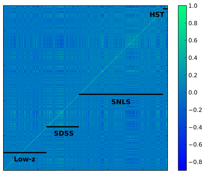
A plot of the full covariance matrix (constructed using flat $\displaystyle w=\mathrm{const}$ model best-fit values $\displaystyle\alpha_{s}=1.43$ and $\displaystyle\beta_{c}=3.26$) is shown in Fig. 2.

To produce the combined constraints in this paper, we include information from both BAO and the CMB in addition to the SN data. In each case, we choose for simplicity distilled quantities which depend only on $\displaystyle\Omega_{M}$, $\displaystyle\Omega_{\mathrm{DE}}$, $\displaystyle\Omega_{K}$, and a parametrized $\displaystyle w(z)$.

For BAO, we compare the theoretical prediction for the acoustic parameter $\displaystyle A(z)$ with the measured value, where we define (see Eisenstein et al. [26])

We combine recent measurements of $\displaystyle A(z)$ at different effective redshifts, using data from the 6dF Galaxy Survey [27], the Sloan Digital Sky Survey (SDSS) Data Release 7 (DR7) [28], the WiggleZ survey [29, 30], and the SDSS Baryon Oscillation Spectroscopic Survey (BOSS) [31, 32]. The measured values are summarized in Table 2.

A plot of the measured values and their uncertainties superimposed on an $\displaystyle A(z)$ curve (Fig. 3) suggests that there is no significant tension between the measurements. Note that the SDSS DR7 measurements at $\displaystyle z=(0.2,0.35)$ are correlated with correlation coefficient 0.337. The WiggleZ measurements are correlated with coefficient 0.369 for the pair $\displaystyle z=(0.44,0.6)$ and coefficient 0.438 for $\displaystyle z=(0.6,0.73)$. Ignoring the relatively small overlap in survey volume between SDSS DR7 and the BOSS sample, we expect all other pairwise correlations to be zero. We compute $\displaystyle\chi^{2}$ in the usual way for correlated measurements, as in Eq. (2).

Nearly all of the sensitivity of the CMB to DE comes from the measurement of an angle at which the sound horizon at $\displaystyle z\approx 1100$ is observed (e.g. [33]). This measurement in turn determines the angular diameter distance to recombination with the physical matter quantity, $\displaystyle\Omega_{M}h^{2}$, essentially fixed. The latter quantity is popularly known as the CMB shift parameter $\displaystyle R$ and is defined as

where $\displaystyle z_{\ast}=1091.3$ is the redshift of decoupling as measured by WMAP7 [34] and $\displaystyle r(z)$ is the comoving distance to redshift $\displaystyle z$. We take the measured value of $\displaystyle R$ to be the value determined by WMAP7, $\displaystyle R_{0}=1.725\,\pm\,0.0184$ [34]. We compute $\displaystyle\chi^{2}$ in the usual way, comparing this measured value of $\displaystyle R$ with the theoretical prediction.

Calculating the combined SN, BAO, and CMB likelihood is now a simple task. We define $\displaystyle\mathcal{L}_{\mathrm{comb}}\propto e^{-\chi^{2}_{\mathrm{tot}}/2}$, where $\displaystyle\chi^{2}_{\mathrm{tot}}=\chi^{2}_{\mathrm{SN}}+\chi^{2}_{\mathrm{BAO}}+\chi^{2}_{\mathrm{CMB}}$.

We use two alternate codes to produce our constraints. For the basic constraints, including the constant equation of state of DE or the $\displaystyle(w_{0},w_{a})$ description, we use a brute-force search which computes likelihoods over a grid of values of $\displaystyle\sim\,$5 parameters (listed below).

Alternatively, we developed a new Markov Chain Monte Carlo (MCMC; e.g. see [35, 36]) code to determine DE parameter constraints and figures of merit (FoMs) for the general ($\displaystyle\sim\,$13 parameters) PC description. The MCMC procedure is based on the Metropolis-Hastings algorithm [37, 38]. From the likelihood $\displaystyle\mathcal{L}(\mathbf{x}|\mathbf{\theta})$ of the data $\displaystyle\mathbf{x}$ given each proposed parameter set $\displaystyle\mathbf{\theta}$, Bayes’ Theorem tells us that the posterior probability distribution of the parameter set given the data is

where $\displaystyle\mathcal{P}(\mathbf{\theta})$ is the prior probability density. The MCMC algorithm generates random draws from the posterior distribution. We test convergence of the samples to a stationary distribution that approximates $\displaystyle\mathcal{P}(\mathbf{\theta}|\mathbf{x})$ by applying a conservative Gelman-Rubin criterion [39] of $\displaystyle R-1\lesssim 0.03$ across a minimum of four chains for each model class. We use the getdist routine of the CosmoMC code [40, 41] to process the resulting chains; getdist bins the chains and then smoothes the binned distribution of counts by convolution with a multidimensional Gaussian kernel.

We verified that the two codes give results that are in excellent agreement in several relevant cases, e.g. constraints in the $\displaystyle\Omega_{M}$–$\displaystyle w$ or $\displaystyle w_{0}$–$\displaystyle w_{a}$ plane.

Before beginning our discussion of systematics, we briefly consider the vanilla $\displaystyle\Lambda\mathrm{CDM}$ cosmology, where $\displaystyle w=-1$. The cosmological parameters describing the expansion rate are matter and cosmological constant densities relative to critical, $\displaystyle\Omega_{M}$ and $\displaystyle\Omega_{\Lambda}$. Including the nuisance parameters, the total parameter set is

We combine SN constraints with BAO and CMB constraints and marginalize over the other parameters to map the likelihood of $\displaystyle\Omega_{\Lambda}$. We find a mean value $\displaystyle\Omega_{\Lambda}=0.724\,\pm\,0.0114$. This suggests that a universe with zero (or negative) cosmological constant is ruled out at approximately 64-$\displaystyle\sigma$! Amusingly, using the brute-force likelihood search that includes the positive and negative values of $\displaystyle\Omega_{\Lambda}$, we find that the combined data give a remarkably low likelihood of zero or negative vacuum energy, even allowing for nonzero curvature: $\displaystyle P(\Omega_{\Lambda}\leq 0)\sim 10^{-267}$. Of course, in reality, the evidence for DE is not nearly this convincing, since the likelihood in the space of cosmological observables is certainly not expected to be Gaussian this far away from the peak and thus would not be described by $\displaystyle\mathcal{L}_{\mathrm{comb}}\propto e^{-\chi^{2}_{\mathrm{tot}}/2}$ (we discuss a related issue in Sec. IV). Nonetheless, it is impressive how strong the evidence for DE is with current data.

We now discuss how one goes beyond $\displaystyle\Lambda\mathrm{CDM}$ cosmology by parametrizing the DE equation of state.

Previous work on the effect of systematics, such as [5], considered the DE sector parametrized by its energy density relative to critical, $\displaystyle\Omega_{\mathrm{DE}}$, and a constant equation of state $\displaystyle w$. Here, we are particularly interested in extending the DE sector to allow for a time-varying equation of state. We make two alternative choices in addition to the constant equation of state so that the three parametrizations we consider are:

1. 1.

   Constant equation of state, $\displaystyle w=\mathrm{constant}$;

2. 2.

   Equation of state described with $\displaystyle w_{0}$ and $\displaystyle w_{a}$ [42], so that $\displaystyle w(a)=w_{0}+w_{a}(1-a)$;

3. 3.

   Equation of state described by a finite number of principal components of $\displaystyle w(z)$ [43].

We now describe in more detail the different parametrizations of DE that we consider (constant $\displaystyle w$, $\displaystyle w_{0}$ and $\displaystyle w_{a}$, PCs) and then proceed to analyze the effects of SN systematics on parameter constraints.

Assuming that DE can be described by an equation of state $\displaystyle w$ that is constant in time, and assuming a flat universe, we calculate the SN-only likelihood in the $\displaystyle\Omega_{M}$–$\displaystyle w$ plane. We marginalize over the usual nuisance parameters $\displaystyle\mathcal{M}$, $\displaystyle\alpha_{s}$, and $\displaystyle\beta_{c}$.

The results for SN-only constraints on $\displaystyle\Omega_{M}$ and $\displaystyle w$ are shown in Fig. 4, where we illustrate the effect of the systematics by showing constraints from the full covariance matrix $\displaystyle\mathbf{C}^{\mathrm{full}}$ on top of those which assume only the diagonal statistical uncertainties $\displaystyle\mathbf{D}^{\mathrm{stat}}$. The systematic uncertainties broaden the well-determined direction in the $\displaystyle\Omega_{M}$-$\displaystyle w$ plane without elongating the poorly determined direction much. Constraints in either parameter are not appreciably shifted. The marginalized uncertainty for $\displaystyle w$ is $\displaystyle\sigma_{w}=0.17$ for diagonal errors only and $\displaystyle\sigma_{w}=0.20$ when systematic errors are included. Thus systematic errors increase the uncertainty by about 20%.

We also seek to understand how SN systematics influence the stretch and color parameters $\displaystyle\alpha_{s}$ and $\displaystyle\beta_{c}$, not only because these correlations are what make SNe Ia useful standard candles, but also because it is expected that systematics could potentially affect these correlations. In Fig. 5, we marginalize over $\displaystyle\mathcal{M}$, $\displaystyle\Omega_{M}$, and $\displaystyle w$ to show constraints on the stretch and color coefficients $\displaystyle\alpha_{s}$ and $\displaystyle\beta_{c}$. Of particular interest is the color coefficient $\displaystyle\beta_{c}$, which is broadly consistent with values found previously; the systematic errors shift it slightly upwards and increase errors in both parameters by a modest amount.

We wish to understand the constraints on the redshift dependence of $\displaystyle w(z)$, so we allow $\displaystyle w(z)$ to have the form [42, 44]

Constraints on $\displaystyle w_{0}$ and $\displaystyle w_{a}$ in a flat universe are shown in Fig. 6. The shaded blue contours represent constraints with only statistical SN errors assumed ($\displaystyle\mathbf{D}^{\mathrm{stat}}$), while the red contours include the full systematic SN covariance matrix ($\displaystyle\mathbf{C}^{\mathrm{full}}$). The left panel shows SN-only constraints, while the right panel shows constraints when BAO and CMB information is also included.

The figure of merit (FoM) for this model defined by the Dark Energy Task Force (DETF) [45, 46] is the inverse of the area of the 95.4% confidence level region $\displaystyle A_{95}$ in the $\displaystyle w_{0}$–$\displaystyle w_{a}$ plane. To be precise about its normalization, we simply define the FoM as in Mortonson et al. [15] as

The approximate equality in Eq. (12) becomes exact for a Gaussian posterior distribution. The FoMs for various scenarios in the $\displaystyle w_{0}$–$\displaystyle w_{a}$ plane are given in Table 3. We find that including the systematic errors reduces the FoM by about a factor of two to three.

We now describe the methodology of how to calculate and constrain the principal components of DE [43], which are weights in redshift ordered by how well they are measured by a given cosmological probe and with a given survey.

Following e.g. Mortonson et al. [14], we first precompute the PCs assuming the current data centered at a fixed fiducial model (we choose the standard flat $\displaystyle\Lambda\mathrm{CDM}$ model with $\displaystyle\Omega_{M}=1-\Omega_{\Lambda}=0.25$). We follow the procedure set forth by the Figure of Merit Science Working Group (FoMSWG) [47] and parametrize $\displaystyle w(z)$ by 36 piecewise constant values in bins uniformly spaced in scale factor $\displaystyle a$ in the range $\displaystyle 0.1\leq a\leq 1.0$. We fix (i.e. ignore) all other parameters in the FoMSWG except for $\displaystyle\Omega_{M}$ and the SN Ia nuisance parameter³³ 3 In the Fisher matrix precomputation of the PCs we assume a single $\displaystyle\mathcal{M}$ parameter as per usual practice (and following the FoMSWG parametrization), but in the actual constraints on the cosmological parameters we adopt two such parameters as described in Sec. II.1. To the extent that the PCs will be correlated anyway due to the differences between real data and assumed “data” going into the Fisher matrix, this subtle difference will be unimportant. $\displaystyle\mathcal{M}$ because they are not probed by the SN Ia data, and at the same time they are effectively marginalized over in the BAO and CMB data in the distilled observable quantities, $\displaystyle A(z)$ and $\displaystyle R$ respectively, that we use. We fix curvature to zero.

We therefore have a $\displaystyle 38\times 38$ Fisher matrix (or really a $\displaystyle 45\times 45$ Fisher matrix with seven parameters fixed), corresponding to parameters

We marginalize over $\displaystyle\Omega_{M}$ and $\displaystyle\mathcal{M}$ and then diagonalize the remaining $\displaystyle 36$-dimensional Fisher matrix of the piecewise constant $\displaystyle w$ parameters. The resulting eigenvectors – shapes that describe $\displaystyle w(z)$ – are the PCs $\displaystyle e_{i}(z)$, and we show the 10 best-determined of these PCs, $\displaystyle e_{1}(z)$–$\displaystyle e_{10}(z)$, in Fig. 7.

The equation of state can be described as [48]

where $\displaystyle\alpha_{i}$ are amplitudes for each PC $\displaystyle e_{i}(z)$. While the Fisher matrix tells us the best accuracy to which these PCs are measured using the assumed data set (these accuracies are related to the eigenvalues $\displaystyle\lambda_{i}$ via $\displaystyle\sigma(\alpha_{i})=\lambda_{i}^{-1/2}$), we are not interested in this; rather, we would like to constrain the PCs using actual current data.

We then feed the shapes in redshift of the first several PCs to the MCMC procedure to constrain these (and a few other, non-$\displaystyle w(z)$) parameters.

Finally, in our parameter search we impose weak priors on the PCs. Following [48] we impose a hard-bound prior on each $\displaystyle\alpha_{i}$, enforcing its contribution to excursions in the equation of state to the region $\displaystyle|1+w(z)|\leq 1$. This approach yields top-hat priors of width [15]

centered at $\displaystyle w(z)=-1$ or $\displaystyle\alpha_{i}=0$. As we will demonstrate, these priors are much wider than the allowed ranges for most of the individual PCs, meaning that our principal results are largely unaffected by the prior (Indeed, we verified this explicitly by constraining the PCs without the prior).

The pairwise constraints on all 13 parameters ($\displaystyle\Omega_{M}$, the PC amplitudes $\displaystyle\alpha_{1}-\alpha_{10}$, and the nuisance parameters $\displaystyle\alpha_{s}$ and $\displaystyle\beta_{c}$) are shown in Fig. 8. The black curves represent constraints from the diagonal statistical SN errors only, while the red curves correspond to the full SN covariance matrix. Overall, the systematic errors broaden and shift the contours slightly.

In Fig. 9, we show the individual marginalized constraints on the 10 PC amplitudes. We are extremely encouraged by the fact that constraints on more than five of the lowest PCs are very good even with current data, a result incidentally also found by [14] using a slightly different combined “current” data set that, most notably, did not include the BOSS and WiggleZ BAO measurements. Here we again see that the SN systematics broaden the constraints slightly; however, as we show just below, the cumulative effect of the systematics on the FoM is not negligible.

We finally calculate the generalization of the DETF FoM to PCs. As defined in Mortonson et al. [15],

where $\displaystyle\mathbf{C}_{n}$ is the $\displaystyle n\times n$ covariance submatrix of $\displaystyle n$ PCs and

is the determinant of the top-hat prior covariance on the $\displaystyle n$ PC coefficients. Each $\displaystyle(\Delta\alpha_{i}/\sqrt{12})^{2}$ term refers to the RMS value of the top-hat prior, where $\displaystyle\Delta\alpha_{i}$ is the width of the top-hat prior as calculated in Eq. (15).

FoM results are shown in Fig. 10, where we show the FoM as a function of the number of PCs included. The top panel shows the FoMs with and without SN systematic errors, while the bottom panel shows the corresponding ratios of the two cases. We see that the FoM degradation with the addition of SN systematic errors asymptotes to about a factor of two when only two PCs are included and after that remains relatively constant. We therefore conclude that only the lowest two PCs are affected by current systematic errors. We suspect that this is due to the fact that the effect of the systematics is smooth in redshift, and therefore systematics do not become degenerate with the higher PCs that wiggle in $\displaystyle z$ (see the PC shapes in Fig. 7). It is somewhat fortuitous that higher ($\displaystyle n>2$) PCs seem to be unaffected by systematics, since it is precisely those higher PCs that are difficult to measure accurately; however, it may be the case that systematics in future data will behave differently and affect the higher components.

References

- [1] A. G. Riess et al., Astron. J. 116, 1009 (1998), astro-ph/9805201 .
- [2] S. Perlmutter et al., Astrophys. J. 517, 565 (1999), astro-ph/9812133 .
- [3] J. Frieman, M. Turner, and D. Huterer, Ann. Rev. Astr. Astrophys. 46, 385 (2008), arXiv:0803.0982 .
- [4] D. H. Weinberg, M. J. Mortonson, D. J. Eisenstein, C. Hirata, A. G. Riess, et al., (2012), arXiv:1201.2434 .
- [5] A. Conley, J. Guy, M. Sullivan, N. Regnault, P. Astier, et al., Astrophys.J.Suppl. 192, 1 (2011), arXiv:1104.1443 .
- [6] W. M. Wood-Vasey et al., Astrophys. J. 666, 694 (2007), astro-ph/0701041 .
- [7] M. Hicken et al., Astrophys. J. 700, 1097 (2009), arXiv:0901.4804 .
- [8] R. Kessler et al., Astrophys. J. Suppl. 185, 32 (2009), arXiv:0908.4274 .
- [9] M. Sullivan, J. Guy, A. Conley, N. Regnault, P. Astier, et al., Astrophys.J. 737, 102 (2011), arXiv:1104.1444 .
- [10] T. M. Davis, E. Mortsell, J. Sollerman, A. Becker, S. Blondin, et al., Astrophys.J. 666, 716 (2007), astro-ph/0701510 .
- [11] D. Rubin, E. Linder, M. Kowalski, G. Aldering, R. Amanullah, et al., Astrophys.J. 695, 391 (2009), arXiv:0807.1108 .
- [12] R. Amanullah, C. Lidman, D. Rubin, G. Aldering, P. Astier, et al., Astrophys.J. 716, 712 (2010), arXiv:1004.1711 .
- [13] N. Suzuki, D. Rubin, C. Lidman, G. Aldering, R. Amanullah, et al., Astrophys.J. 746, 85 (2012), arXiv:1105.3470 .
- [14] M. J. Mortonson, W. Hu, and D. Huterer, Phys. Rev. D81, 063007 (2010a), arXiv:0912.3816 .
- [15] M. Mortonson, W. Hu, and D. Huterer, Phys. Rev. D82, 063004 (2010b).
- [16] D. Huterer and A. Cooray, Phys. Rev. D71, 023506 (2005), astro-ph/0404062 .
- [17] Y. Wang and M. Tegmark, Phys. Rev. D71, 103513 (2005), astro-ph/0501351 .
- [18] C. Zunckel and R. Trotta, Mon. Not. Roy. Astron. Soc. 380, 865 (2007), astro-ph/0702695 .
- [19] G.-B. Zhao, D. Huterer, and X. Zhang, Phys. Rev. D77, 121302 (2008), arXiv:0712.2277 .
- [20] A. Hojjati, L. Pogosian, and G.-B. Zhao, JCAP 1004, 007 (2010), arXiv:0912.4843 .
- [21] E. E. Ishida and R. S. de Souza, Astron.Astrophys. 527, A49 (2011), arXiv:1012.5335 .
- [22] A. Shafieloo, A. G. Kim, and E. V. Linder, (2012), arXiv:1204.2272 .
- [23] M. Seikel, C. Clarkson, and M. Smith, JCAP 1206, 036 (2012), arXiv:1204.2832 .
- [24] G.-B. Zhao, R. G. Crittenden, L. Pogosian, and X. Zhang, (2012), arXiv:1207.3804 .
- [25] J. Guy, P. Astier, S. Baumont, D. Hardin, R. Pain, et al., Astron.Astrophys. 466, 11 (2007), astro-ph/0701828 .
- [26] D. J. Eisenstein et al., Astrophys. J. 633, 560 (2005), astro-ph/0501171 .
- [27] F. Beutler, C. Blake, M. Colless, D. H. Jones, L. Staveley-Smith, et al., Mon.Not.Roy.Astron.Soc. 416, 3017 (2011), arXiv:1106.3366 .
- [28] W. J. Percival et al. (SDSS Collaboration), Mon.Not.Roy.Astron.Soc. 401, 2148 (2010), arXiv:0907.1660 .
- [29] C. Blake, S. Brough, M. Colless, C. Contreras, W. Couch, et al., (2012), arXiv:1204.3674 .
- [30] C. Blake, E. Kazin, F. Beutler, T. Davis, D. Parkinson, et al., Mon.Not.Roy.Astron.Soc. 418, 1707 (2011), arXiv:1108.2635 .
- [31] A. G. Sanchez, C. Scoccola, A. Ross, W. Percival, M. Manera, et al., (2012), arXiv:1203.6616 .
- [32] L. Anderson, E. Aubourg, S. Bailey, D. Bizyaev, M. Blanton, et al., (2012), arXiv:1203.6594 .
- [33] J. A. Frieman, D. Huterer, E. V. Linder, and M. S. Turner, Phys. Rev. D67, 083505 (2003), astro-ph/0208100 .
- [34] E. Komatsu et al. (WMAP), Astrophys. J. Suppl. 192, 18 (2011), arXiv:1001.4538 .
- [35] N. Christensen, R. Meyer, L. Knox, and B. Luey, Class. Quant. Grav. 18, 2677 (2001), astro-ph/0103134 .
- [36] J. Dunkley, M. Bucher, P. G. Ferreira, K. Moodley, and C. Skordis, MNRAS 356, 925 (2005), astro-ph/0405462 .
- [37] N. Metropolis, A. Rosenbluth, M. Rosenbluth, A. Teller, and E. Teller, J.Chem.Phys. 21, 1087 (1953).
- [38] W. Hastings, Biometrika 57, 97 (1970).
- [39] A. Gelman and D. Rubin, Statistical Science 7, 452 (1992).
- [40] A. Lewis and S. Bridle, Phys. Rev. D66, 103511 (2002), astro-ph/0205436 .
- [41] http://cosmologist.info/cosmomc/.
- [42] E. V. Linder, Phys. Rev. Lett. 90, 091301 (2003), astro-ph/0208512 .
- [43] D. Huterer and G. Starkman, Phys. Rev. Lett. 90, 031301 (2003), astro-ph/0207517 .
- [44] M. Chevallier and D. Polarski, Int. J. Mod. Phys. D10, 213 (2001), gr-qc/0009008 .
- [45] A. Albrecht et al., (2006), astro-ph/0609591 .
- [46] D. Huterer and M. S. Turner, Phys. Rev. D64, 123527 (2001), astro-ph/0012510 .
- [47] A. J. Albrecht et al., (2009), arXiv:0901.0721 .
- [48] M. J. Mortonson, W. Hu, and D. Huterer, Phys. Rev. D79, 023004 (2009), arXiv:0810.1744 .
- [49] B. A. Bassett and N. Afshordi, (2010), arXiv:1005.1664 .
- [50] R. Kessler, B. Bassett, P. Belov, V. Bhatnagar, H. Campbell, et al., Publ.Astron.Soc.Pac. 122, 1415 (2010), arXiv:1008.1024 .
- [51] R. Hlozek, M. Kunz, B. Bassett, M. Smith, J. Newling, et al., Astrophys.J. 752, 79 (2012), arXiv:1111.5328 .