Computing the refined stability condition
Abstract.
The classical (inviscid) stability analysis of shock waves is based on the Lopatinskiĭ determinant, —a function of frequencies whose zeros determine the stability of the underlying shock. A careful analysis of shows that in some cases the stable and unstable regions of parameter space are separated by an open set of parameters. Zumbrun and Serre [Indiana Univ. Math. J., 48 (1999) 937–992] have shown that, by taking account of viscous effects not present in the definition of , it is possible to determine the precise location in the open, neutral set of parameter space at which stability is lost. In particular, they show that the transition to instability under suitably localized perturbations is determined by an “effective viscosity” coefficient. Here, in the simplest possible setting, we propose and implement two new approaches toward the practical computation of this coefficient. Moreover, in a special case, we derive an exact solution of the relevant differential equations.
Key words and phrases:
Evans function, multidimensional viscous conservation laws, spectral stability1991 Mathematics Subject Classification
35P15, 35B40, 47A451. Introduction
1.1. Inviscid stability
Consider a planar shock solution,
| (1.1) |
of a hyperbolic system of conservation laws in space dimensions:
| (1.2) |
Here, the unknown belongs to , the state space, and is a function of space and time . The fluxes are -valued functions on . In (1.1), are constant states; they are related to the shock speed by the Rankine–Hugoniot condition
where—here and below—square brackets indicate the jump. That is, for any function of the state , . The linear stability analysis of such solutions is now classical; it originates in the studies of pioneers D\cprimeyakov [6] and Erpenbeck [7]. We recall that the the centerpiece of the analysis is the Lopatinskiĭ determinant,
a function of frequencies , where is dual to time and is dual to the transverse spatial directions. Zeros of with correspond to perturbations which grow exponentially in time, and, evidently, nonvanishing of on is necessary for (linearized, inviscid) stability of the shockaa a Indeed, is homogenous degree one. Thus, any unstable zero generates instabilities of all orders. That is, any such instability is of Hadamard type; these instabilities are so violent that these waves will never be seen in practice..
A particularly important example occurs when (1.2) is the Euler equations of gas dynamics and the solution (1.1) represents a planar gas-dynamical shock wave. In this example, the vector would have as its components the mass density, the momentum densities in each of the spatial directions, and the total energy density. In this case, an analysis of , see [5] or the appendix of [14], yields clean, explicit stability criteria in terms of the basic properties of the shock and the gasbb b The stability criteria are, naturally, formulated in terms of the end states of the shock and in terms of the equation of state. in question. However, Majda [9] has observed that in the setting of gas dynamics it sometimes happens that vanishes on the boundary but not for , and in this case we say that the shock is neutrally or weakly stable. Moreover, this neutral stability can persist on an open set in parameter space. Physically, the presence of neutral zeros of corresponds to surface or boundary waves, and these zeros are associated with a loss of smoothness of the perturbed shock front. Further complicating matters, Barmin & Egorushkin [2] have pointed out that experimentally observed instabilities of gas-dynamical shocks sometimes occur within the region of weak stability. That is, instabilities are sometimes observed in the interior of the weakly stable regime. They postulated that the inclusion of nonlinear effects and/or other neglected physical effects would be required for the theory to capture the phenomena revealed by these experiments.
1.2. Viscous stability
By considering the viscous regularization of (1.2),
| (1.3) |
Zumbrun & Serre [12] have shown that the precise location of the transition to instability is entirely determined by viscous effects which are neglected in the construction of . See also the more recent paper of Benzoni-Gavage, Serre, & Zumbrun [4]; this latter paper forms the foundation of the calculations we present herecc c Also, the original, one-dimensional () derivation appears in [3].. As a point of reference, we note that in the aforementioned example of gas dynamics, equation (1.3) would correspond to the Navier–Stokes equations of compressible gas dynamics; the second-order terms on the right-hand side of (1.3) model the effects of viscosity and heat conductivity.
We associate to the solution (1.1) of the inviscid equations (1.2) a planar viscous profile for (1.3). The viscous profile is a solution of (1.3) of the form
| (1.4) |
Zumbrun & Serre’s derivation is based on a low-frequency analysis of the Evans function, , associated with (1.4). Analogous to the Lopatinskiĭ determinant, the Evans function is a spectral determinant; its zero set carries stability information for the planar viscous shock wave. In particular, the refined stability condition they derive is given in terms of the sign of the real part of a coefficient called ; see (3.38) below. That is,
is a necessary condition for weak viscous stability. Our principal aim here is to explore, in a simplified setting, the effective, practical computation of . As pointed out by Benzoni-Gavage, Serre, & Zumbrun [4], the fundamental challenge for computing is the numerical approximation of the function , the solution of an appropriate differential equation; see (3.40) below. The determination of has been identified as an important open problem for physical systems due its possible role as a signal for the onset of complex behavior [13]; see also Zumbrun’s more recent work on the role of the refined stability condition in the development of cellular instabilities for shock waves [16].
1.3. Plan
In §2 we describe the framework that we use as a testbed for computing (and therefore ). In particular, we restrict our attention to the case of a scalar conservation law with viscosity in two space dimensions. In §3, for completeness and to make the exposition here mostly self contained, we recapitulate the derivation of and related Evans-function analysis from [4]; notably, because we have restricted ourselves to the scalar case, our derivation is substantially streamlined from the general calculation presented there. In §4 we make the principal contribution of this paper. We propose two distinct approaches toward computing , and we implement these approaches in several concrete example problems. In a special case, we are able to find an exact solution. We use this exact solution to validate our numerical approximations. Finally, in §5 we actually compute and discuss the steps that will be required to compute using these or similar techniques in the interesting (and physically relevant!) system case. These calculations represent, to the best of our knowledge, the first ever calculations of the refined stability condition in any setting.
2. Preliminaries
2.1. Model
We consider the simplest possible scenario of interest, a single conservation law with viscosity in two space dimensions:
| (2.1) |
Here, is real valued, , and represents time. We shall write . The parameter is the viscosity; for simplicity we shall take . Equation (2.1) is the viscous correction of the hyperbolic conservation law
| (2.2) |
Evidently, (2.2) is hyperbolic since the matrix is always real for . As is well known, such systems support discontinuous solutions (shocks), and we consider here the simplest possible shock solution, a planar shock wave connecting constant states. That is, we suppose as above that
| (2.3) |
is a solution of (2.2). We recall that, in order for to be a weak solution of (2.2), and must satisfy the Rankine–Hugoniot condition
| (2.4) |
2.2. Lopatinskiĭ determinant
Applying the classical stability analysis to amounts to the algebraic construction of the Lopatinskiĭ determinant . In general, i.e., in the case of (1.2), is constructed from a jump term
together with bases for the stable () and unstable () subspaces of the matrices
| (2.5) |
For a Lax -shock, the dimensions work out precisely since in that case
However, in our setting (, ), the Lopatinskiĭ determinant consists only of the jump term, and we can write it down explicitly as
| (2.6) |
First, observe that provided , there are no zeros of with . Evidently, given a pair of states and a flux function , it is always possible to find a purely imaginary value of for which vanishes. Namely, one can simply take
The fact that there is a whole line of neutral zeros parametrized by is a manifestation of the homogeneity of .
Remark 1.
The above calculation shows that planar shocks for (2.2) are always weakly stable; see the discussion in [5]. Thus, in the current setting, the goal of computing of could be regarded as artificial because it does not—in this case—serve to locate the transition point in parameter space separating the (strongly) stable and unstable regions. On the other hand, the simple form of in (2.6) and the resulting abundance of weakly stable shocks makes this setting ideal for testing various approaches to the computation of . The extension of these ideas to a physically relevant case with is part of our ongoing work [1]; in §5.2 we indicate some features of our computations which might be useful in the setting of systems.
2.3. Traveling-wave solutions
We now turn to the equation with viscosity. Recall, we have set , and we seek solutions of (2.1) of the form
| (2.7) |
We write , and we note that the traveling-wave ansatz (2.7) reduces the partial differential equation (2.1) to
| (2.8) |
Integrating (2.8) once, we find
| (2.9) |
A necessary condition for the existence of a traveling-wave profile is that both states be equilibria of the equation (2.9). Evidently, is an equilibrium. From the requirement that be an equilibrium we recover the Rankine–Hugoniot condition (2.4):
Example 2 (Burgers flux).
In the case that , the Rankine–Hugoniot condition (2.4) reduces to
so the shock speed is simply the average of the values of the end states. We take
so that . Equation (2.9) reduces in this case to
| (2.10) |
and a straightforward and well-known calculation shows that We shall use this exact solution of the profile equation (2.10) to validate our numerical calculations below. See also Example 12 below.
We note that the two Lax shock conditions
| (2.11) |
guarantee that the equilibrium at is a stable node and that the equilibrium at is an unstable node. Thus, since the phase space for the nonlinear differential equation is one dimensional, provided that there are no equilibria between and , existence of a monotone profile is immediate. Moreover, the profile will approach its limiting values exponentially fast.
Remark 3.
By a modification of the flux if necessary, we may assume that . We make this assumption throughout the remainder of the paper. Thus, from this point forward the profile is a standing wave, a function of alone.
2.4. Linearization
The first step in the stability analysis is to linearize (2.1) about the standing-wave solution . We obtain
| (2.12) |
Here, denotes the perturbation, and equation (2.12) describes the approximate (linear) evolution of the perturbation . In particular, if the linearized equation supports solutions which grow in time, the solution will be unstable. The linear equation (2.12) has variable coefficients (since is nonconstant), but these coefficients are functions of alone. Thus, we may take the Laplace transform in (dual variable ) and the Fourier transform in (dual variable ). The transformed equation, with denoting the transformed perturbation, takes the form
| (2.13) |
Here, ′ denotes differentiation with respect to . Indeed, from this point forward, we omit the superfluous subscript on ; it is the only surviving spatial variable. Thus, will denote the spatial coordinate normal to the unperturbed shock front. We think of (2.13) as a family of eigenvalue problems for the collection of linear operators parametrized by and defined by
| (2.14) |
We sometimes write as a convenient shorthand for (2.13). Solutions of which decay at with correspond to perturbations which grow in time since can be recovered from via
Evidently, since as , there are a pair of related, limiting operators
| (2.15) |
Notably, for every the operators are constant-coefficient operators. Thus, they may be analyzed quite completely. This feature is an essential ingredient of the analysis. We also note for future reference that
and, evidently, from (2.8) with , we find
| (2.16) |
Thus, is a decaying solution of (2.13) corresponding to .
3. Evans function
3.1. Evans function and low-frequency limit
The Evans function is easily constructed in this case. We content ourselves with a mere outline of the procedure here. For more details in a setting which includes ours as a special case, see [12, 4] . First, we rewrite the eigenvalue problem as a first-order system of differential equations:
| (3.1) |
As above, we use ′ to denote differentiation with respect to , and we have written . The coefficient matrix is given by
| (3.2) |
Corresponding to the constant coefficient operators , there are constant coefficient first-order systems with
| (3.3) |
The eigenvalues of are roots of
| (3.4) |
Observe that as long as there can be no imaginary root of (3.4). To see this, simply observe that if for , then the left-hand side of (3.4) has as its real part the expression
which is clearly negative provided that . Thus, the matrices have no center subspace on , and one can therefore determine the dimensions of the stable and unstable subspaces of by taking . Consideration of (3.4) then shows that the stable and unstable subspaces of the two matrices each have dimension one on . Of particular interest are the stable subspace and the unstable subspace . The next lemma shows that there are solutions of the variable-coefficient problem (3.1) which asymptotically tend to zero (forward or backward in ) in the directions of these invariant subspaces.
Lemma 4.
Fix a base point . There exist solutions of (3.1) such that
Local to , these solutions are holomorphic in and real analytic in .
Proof.
The proof is a consequence of the preceding constant-coefficient analysis and the conjugation lemma of [10]. In particular, the conjugation lemma asserts the existence of a well-behaved invertible change of coordinates which maps solutions of the constant-coefficient problem to solutions of the variable-coefficient one. See [12] for details. ∎
Definition 5 (Evans function).
The (local) Evans function is defined by
| (3.5) |
Our principal interest is in the polar Evans function defined for radial coordinate by
For ease of notation, we sometimes suppress the dependence on and and simply denote the Evans function by .
Remark 6.
The key point is to understand what happens when and when . In general, a delicate issue that arises on the boundary of are the glancing and variable multiplicity sets and . However, when , a direct computation shows that
Thus, we need not concern ourselves with these sets here. In the general case, the presence of glancing points, for example, prohibits the smooth extension of the stable and unstable subspaces of to , and these points—a measure zero set—must be excised from the boundary of in advance of the low-frequency analysis of that follows. See [4] or [15] for more details.
The next lemma paves the way for the fundamental low-frequency analysis of that is the cornerstone of the derivation of . We omit the proof which is technical; details can be found in [12].
Lemma 7 (Low-frequency extension).
Fix a base point . The Evans function and its factors have a unique jointly analytic extension onto a neighborhood of . Moreover, the factors may be chosen so that
with and .
With Lemma 7 in hand, we are ready to outline the proof of the fundamental result of Zumbrun & Serre [12]. Importantly, it links in a rigorous way the Lopatinskiĭ determinant encoding the stability of the inviscid, ideal shock (2.3) and the Evans function associated with the corresponding viscous profile (2.7). Roughly speaking, the result says that low-frequency/long-wave perturbations cannot distinguish between the inviscid, ideal shock and the viscous profile .
Proposition 8 (Zumbrun & Serre, [12]).
Fix . Then,
| (3.6) |
Here, is a constant measuring transversality of the connection in the traveling-wave problemdd d Transversality is automatic in the case we consider in this paper.. The quadratic error term is uniform for in bounded subsets of . Equivalently, and
| (3.7) |
Proof.
We outline the principal calculation. First, recalling the discussion surrounding equation (2.16), we make the standard normalization at that . From this, the assertion that is immediate. Second, observe that
| (3.8) |
But then, using again the normalization at , we see that the expression for the derivative of the Evans function in (3.8) may be rewritten as
| (3.9) |
where and . In polar coordinates the eigenvalue equation takes the form
| (3.10) |
Thus, differentiating with respect to and setting , we find from (3.10) that
| (3.11) |
We rewrite (3.11) as
| (3.12) |
to express both sides of the equation as perfect derivatives. We integrate the equation in (3.12) from to (Recall, ):
| (3.13) |
Similarly, we integrate the equation from to :
| (3.14) |
Combining the results of (3.13) and (3.14), we find that the components of satisfy the equation
| (3.15) |
But, as we noted above in (2.16), satisfies , or
| (3.16) |
Equations (3.15) and (3.16) show that the row operation of adding times the first row to the second row simplifies the Evans determinant as follows
| (3.17) |
This completes the outline of the proof. ∎
3.2. The building blocks of
In this section we outline the derivation of the final ingredient of ; these calculations provide the framework for our computational approach. They depend on the calculations in §3.1, particularly those in the proof of Proposition 8. The basic assumption is that is a zero of with . In the current setting, this means that and are related via
| (3.18) |
Proposition 9 (Benzoni-Gavage, Serre, & Zumbrun, [4]).
If is a neutral zero of , then
| (3.19) |
Proof.
First, we note that the assumption implies that (see (3.15))
But, this implies that, for some constant ,
Therefore, we define
| (3.20) |
and we note that at , we have
We shall use this new basis for our computations. That is, we now compute with the alternatively defined Evans function
| (3.21) |
The advantage is that, with this new basis,
| (3.22) |
Then, as in Proposition 8, and (now also) . We now examine the second derivative of with respect to . We observe that, by the Leibniz rule, the second derivative of the Evans determinant may be expanded as
| (3.23) |
But, by (3.22), it follows immediately that
Thus, we may proceed in a fashion similarly as in Proposition 8. The two remaining determinants in (3.23) may be combined so that
| (3.24) |
where
| (3.25) |
We differentiate (3.10) twice with respect to and we set ; we find that satisfy the equation
| (3.26) |
or, rearranging terms,
| (3.27) |
But, since , we subtract and integrate in (3.27) to find that satisfies
| (3.28) |
where is a constant. Next, by a row operation as in the proof of Proposition 8, we find that
| (3.29) |
It remains to identify the constant . We define by . That is, the action of on a function is given by
Thus, we may rewrite (3.28) as
| (3.30) |
But, by the fundamental theorem of calculus,
| (3.31) | ||||
| and | ||||
| (3.32) | ||||
Thus, using (3.31) and (3.32), we are finally in a position to identify the constant . We see, starting with the expression in (3.30), that
| (3.33) | ||||
| (3.34) | ||||
| (3.35) | ||||
| (3.36) |
We note that the equality in (3.35) follows from the fact that (see (3.27)), and the boundary terms vanish because tends to zero exponentially as . In conclusion, we have shown that
| (3.37) |
∎
Propositions 8 and 9 provide the fundamental ingredients for the derivation and calculation of . The derivation is based on the relationship between the zero sets of and expressed in Proposition 8. The main analytic tool is the implicit function theorem. We omit the details, which may be found in [12], and simply note that is given by
| (3.38) |
But, Proposition 8 implies that
and—given the explicit form of in (2.6)—we see immediately that
Thus, from Proposition 9, we find that
| (3.39) |
From (3.39) we see immediately that the computation of requires one to compute . Evidently, from (3.37), to compute one needs to know both the profile and the function solving the differential equation (see (3.12))
| (3.40) |
In the next section we propose two methods for the practical approximation of .
Remark 10.
Briefly, the sign of detects whether or not the zero level set of curls into the unstable half plane. Heuristically, it has a physical interpretation as an “effective viscosity” coefficient for transversely propagating deformations of the front. A detailed discussion of this point can be found in [12].
4. Computing
As pointed out in [4], the principal task in finding is to compute ; the other elements required to compute are the building blocks of ---in general these are the eigenvalues and eigenvectorsee e In the general case, one also uses these eigenvalues and eigenvectors to compute a boundary term ; this term does not appear in our setting. of —and the profile . Benzoni-Gavage, Serre, & Zumbrun [4] have proposed a two-step method for finding . That is, the equation for is a linear equation whose coefficients depend on the profile . Thus, they propose to first solve the profile equation (2.9). For gas dynamics, techniques for doing this are well known; see, e.g., [8]. Then, they describe how to transform the equation for into one that fits into a standard numerical framework for approximating the solution of a two-point boundary value problem. Their method has never, to our knowledge, been implemented. Below, we propose two alternative approaches that, at least in the present context (), work well. We are currently investigating all three approaches in the case of gas dynamics for which .
4.1. Integrating factor
This method exploits the linear structure of (3.40). The equation for is
| (4.1) |
We integrate both sides of (4.1), and we obtain
| (4.2) |
We write in terms of its real and imaginary parts as
Then, the relevant system of equations becomes
| (4.3a) | ||||
| (4.3b) | ||||
We suppose that is known, and we write
Now, suppose that is defined by
| (4.4) |
Then, a simple calculation shows that , whence the equation for can be rewritten as a perfect derivative . Integrating from to and using , we find immediately that
| (4.5) |
Thus, is given explicitly in terms of the profile . Similarly, we apply the integrating factor to the equation for . We write , and we see that
| (4.6) |
Equations (4.5) and (4.6) show that we may write explicitly in terms of the profile . Thus, rather than solve a differential equation for , in this case we may simply approximate (as described above, a well understood problem) and then use that approximation to compute the integrals in (4.5) and (4.6). Indeed, as Example 12 below shows, in some cases it is possible to compute these integrals exactly.
Remark 11.
From [4], we note that in the computation of , the two apparently free parameters and above should be chosen so that satisfies an orthogonality condition at the origin. In the current setting, this reduces to the requirement that
Example 12 (Exact solution).
In the case of the Burgers flux , we have seen that if , , then . We have also seen that in this case the profile is given by
Suppose that . We take and so that . Then, system of equations (4.3) reduces to
| (4.7) |
That is, we need to solve
By direct computation, with and , we find immediately from (4.5), (4.6) that
| (4.8) |
This solution is plotted in Figure 2.
Remark 13.
The formulae in [4] are derived in the case of strictly parabolic viscosity. That is, the matrices in (1.3) are assumed to satisfy
| (4.9) |
However, the important physical case of gas dynamics features only a partially parabolic or “real” viscosity. For example, consider the equations of isentropic gas dynamics
| (4.10a) | ||||
| (4.10b) | ||||
where and are the first (“dynamic”) and second viscosity coefficients (assumed here to be constant). The lack of second-order terms on the right-hand side of the conservation of mass equation (4.10a) prevents the system (4.10) from satisfying (4.9); nonetheless, it is clear that the results of [4] extend in a natural way to systems with “real” or partially parabolic viscosity, such as the equations of gas dynamics. It is a rather tedious exercise to derive the equation for in that setting. Remarkably, our preliminary calculations for the system (4.10) show that the equation for can be written as a linear diagonal system [1]; this suggests that the above approach based on integrating factors might be applicable to the corresponding calculation for (4.10).
4.2. Coupled formulation
4.2.1. Description
Rather than solve the problem in two steps (first and then ), we consider now the problem of solving the coupled system for and . Thus, we consider the autonomous system
| (4.11a) | ||||
| (4.11b) | ||||
| (4.11c) | ||||
Our motivation for pursuing this approach is that, if the numerical methods involved do not take explicit advantage of the linear structure of the equation, for modestly sized systems it involves no extra work to solve the coupled system in a single step. On the other hand, the challenge in this case is to construct a suitable guess for the solver. However, once a suitable guess is found, the calculation can take advantage of continuation. For example, if is being moved along the Hugoniot curve, one can use the previously found solution as the initial guess for the next value of ; see Example 16. Based on our experiments, this method works quite well.
We write (4.11) as , where . The desired solution is a heteroclinic orbit in the phase space which connects the equilibria . The linearization is straightforward; we see immediately that
| (4.12) |
Evidently, the eigenvalues of are, with multiplicity three, simply . From (2.11) this gives a connection from a stable node to an unstable node in . We expect then to introduce two parameters to completely parametrize the solutions; as noted in Remark 11, an orthogonality condition will select a particular solution for the computation of .
4.2.2. Numerical Implementation
We truncate the problem to the computational domain . Thus, the system becomes
| (4.13) |
At this point we expect to incorporate projective boundary conditions at . Next, for convenience, we double the variables and rescale the problem to the unit interval. Thus we consider the problem
where and . We also implement the classical phase condition to remove the translational invariance from the problem. Folding over the solution makes it simple to include this as a boundary condition at . Thus, in this case, we use one phase condition, three matching conditions, and two free parameters to determine the solution. The penultimate step is to generate an approximate solution, or a guess. In this case, we generate our guess by solving the corresponding initial-value problem. In practice, since this is a sink-source connection, it is not too difficult to generate a good guess by this method. Once a guess of sufficient quality is found; solutions for nearby parameter values can be found easily by continuation. Finally, we solve the boundary-value problem using MatLab’s routine bvp5c; this is a code that implements the four-stage Lobatto IIIa formula; this is a collocation formula. The collocation polynomial provides a -continuous solution that is fifth-order accurate uniformly in the computational domain . Sample solutions using this procedure are plotted in Figure 1 and Figure 2.
Remark 14.
A natural question concerns the determination of the smallest size of that guarantees that the numerical approximation fully resolves the features of the true problem on . Here, for the model problem that we consider, we are content to do so in an ad hoc way. Since our ultimate interest is in , we merely verify that the value of this quantity is stable as is increased; we take this as evidence that the computation is sufficiently resolved. See Table 1.
4.2.3. Examples
Example 15 (, ).
This is the same as Example 12, and so there is an exact solution available. The system takes the form
| (4.14a) | ||||
| (4.14b) | ||||
| (4.14c) | ||||
The approximate solution computed using the method described in Section 4.2 with is plotted against the exact solution in Figure 2. We note that the 2-norm error between the approximate solution and the exact solution on their common domain is well-controlled by the built-in error control features of bvp5c.
Example 16 (Moving end state).
In this example, we take as before and we take
for the transverse flux . Our aim in this example is to mimic the kind of calculation that one would do in practice, searching for the point in parameter space (e.g., the value of ) at which changes sign. To that end, we systematically increase the value of and recompute the and for each new value of the end state. This is precisely the kind of computation that is well suited for continuation. The results are plotted in Figure 1.
(a)  |
(b) 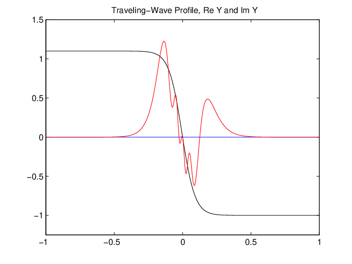 |
(c) 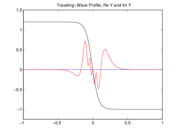 |
(d)  |
(e)  |
(f) |
4.3. Comparison of two methods
In the context of the scalar conservation law (2.1), both methods work well. Our experiments show that some care should be exercised in approximating via the integrating factor method; in particular, the overall quality of the computation depends on the approximation of the integrals in (4.6). Our implementation uses Simpson’s rule to approximate these integrals. It is worth noting that the profile is computed independently in this first method; for example, the calculation does not take any account of the transverse flux . By way of comparison, error control in the coupled formulation is “automatic” since we use built-in convergence tolerances in the package bvp5c to control the quality of the approximation across the entire computational domain; That is, and are treated on the same footing, and this method takes account of the entire structure of the problem at each stage of the iteration. In Figure 2 we plot the exact solution from Example 12 against the approximate solutions obtained by the two methods. The caption of that figure records the error between the approximate solutions and the exact solution in the 2-norm, given by
| (4.15) |
On the other hand, a distinction of note between the methods is in the complexity of the nonlinear two-point boundary-value problem that must be solved. Our technique for solving these problems by collocation hinges on finding or computing a suitable initial guess. This guess is used as the seed in an iterative solution of the nonlinear equations for the coefficients of the collocation polynomial. In the first method, based on the integrating factor, a relatively simple boundary-value problem needs to be solved; one expects that it is, generally, much easier to generate a good initial guess for this problem than to find a similarly good initial guess for the coupled formulation of the problem.

5. Conclusion
5.1. Calculating
Finally, with our approximations of and in hand, we proceed to compute . Examining (3.39), we observe that the formula for may be rewritten as
| (5.1) |
Thus, from §4.1 and §4.2 we have two distinct ways of obtaining approximations for , , and on the computational domain in order to approximate the integral in (5.1). In Table 1 we compare the values of computed by each of the methods for the problem in Example 12. In each case, we approximate the integral in (5.1) by the trapezoid rule, and we denote the different values obtained by and .
| 10 | 20 | 30 | |
|---|---|---|---|
5.2. Discussion
We have considered Zumbrun & Serre’s refined stability condition [12] in the simplest possible setting, and we have proposed and implemented two methods for practically computing the condition. Both methods work well in the present setting, and we believe that the approaches for computing from §4 are potentially useful for interesting physical versions of this problem. Indeed, our principal interest is to use the model problem here as a stepping stone towards the analogous problem for a physical system () which possesses open set of weakly stable waves. For isentropic gas dynamics in two space dimensions (4.10), an example of such a family has been given by Majda [9]. In that case , and the fundamental new issue that arises is the presence of slow modes, see [3, 4]. For example, in the case of a Lax -shock, there are two outgoing characteristic directions, and this alters the calculation from the very beginning. For example, the computation of is more involved (although it is still computable in closed form [11]). In this case the Lopatinskiĭ determinant takes the form
| (5.2) |
where the vectors are a basis for the unstable subspace of where
| (5.3) |
with and
| (5.4) |
In the fluxes , the form of the pressure is prescribed as the equation of state—the constitutive relation that specifies the nature of the gas. Mathematical treatments of gas dynamics frequently take a “-law’’ gasff f Of course, the parameter appearing in (5.5) is a physical constant and is not related to used throughout this paper. Similarly, the gas density appearing in (4.10) and (5.4) is not to be confused with the radial coordinate used in the Evans-function calculations in §3.
| (5.5) |
where is a positive constant and . For such a pressure law, there are no weakly stable shocks [11]. However, thermodynamically admissible perturbations of a -law pressure function can open up regions of weak stability [1, 9]. Additionally, the presence of slow modes introduces an additional boundary term , as described in [4], into the formulation of . The term is associated with the absence of a spectral gap for the linearized operator , and is constructed from the right and left eigenvectors of in (5.3); in the case of (4.10), these are known explicitly. Finally, in the physical cases, low-frequency behavior on can be complicated due to the presence of nonempty glancing and variable multiplicity sets and . In the case of (4.10) is empty and can be computed explicitly. The application of the ideas in §4 to this problem is a topic of our current investigation.
Acknowledgement
Research of all authors was supported in part by the National Science Foundation under grant number DMS-0845127. The authors would also like to thank Mark Ablowitz and Harvey Segur for a helpful suggestion.
References
- [1] (2012) The refined stability condition for gas dynamics. (in preparation). Cited by: §5.2, Remark 1, Remark 13.
- [2] (1992) Stability of shock waves. Adv. Mech. 15 (1-2), pp. 3–37 (English, with English and Russian summaries). External Links: ISSN 1230-0853 Cited by: §1.1.
- [3] (2001) Alternate evans functions and viscous shock waves. SIAM J. Math. Anal. 32 (5), pp. 929–962 (electronic). External Links: ISSN 0036-1410 Cited by: §5.2, footnote c.
- [4] (2008) Transition to instability of planar viscous shock fronts: the refined stability condition. Z. Anal. Anwend. 27 (4), pp. 381–406. External Links: ISSN 0232-2064 Cited by: §1.2, §1.2, §1.3, §3.1, §4, §5.2, §5.2, Remark 11, Remark 13, Remark 13, Remark 6, Proposition 9.
- [5] (2007) Multidimensional hyperbolic partial differential equations. Oxford Mathematical Monographs, The Clarendon Press Oxford University Press. Note: First-order systems and applications External Links: ISBN 978-0-19-921123-4, ISBN 0-19-921123-X Cited by: §1.1, Remark 1.
- [6] (1954) On the stability of shock waves. Ž. Eksper. Teoret. Fiz. 27, pp. 288–295 (Russian). Cited by: §1.1.
- [7] (1962) Stability of step shocks. Phys. Fluids 5, pp. 1181–1187. External Links: ISSN 0031-9171 Cited by: §1.1.
- [8] (2009) Spectral stability of ideal-gas shock layers. Archive for Rational Mechanics and Analysis 194, pp. 1029–1079. Cited by: §4.
- [9] (1984) Compressible fluid flow and systems of conservation laws in several space variables. Applied Mathematical Sciences, Vol. 53, Springer-Verlag. External Links: ISBN 0-387-96037-6 Cited by: §1.1, §5.2, §5.2.
- [10] (2005) Large viscous boundary layers for noncharacteristic nonlinear hyperbolic problems. Mem. Amer. Math. Soc. 175 (826), pp. vi+107. External Links: ISSN 0065-9266 Cited by: §3.1.
- [11] (2000) Systems of conservation laws. 2. Cambridge University Press. Note: Geometric structures, oscillations, and initial-boundary value problems; Translated from the 1996 French original by I. N. Sneddon External Links: ISBN 0-521-63330-3 Cited by: §5.2, §5.2.
- [12] (1999) Viscous and inviscid stability of multidimensional planar shock fronts. Indiana Univ. Math. J. 48 (3), pp. 937–992. External Links: ISSN 0022-2518 Cited by: §1.2, §3.1, §3.1, §3.1, §3.1, §3.2, §5.2, Remark 10, Proposition 8.
- [13] (2001) Multidimensional stability of planar viscous shock waves. pp. 307–516. Cited by: §1.2.
- [14] (2004) Stability of large-amplitude shock waves of compressible navier-stokes equations. pp. 311–533. Note: With an appendix by Helge Kristian Jenssen and Gregory Lyng Cited by: §1.1.
- [15] (2007) Planar stability criteria for viscous shock waves of systems with real viscosity. pp. 229–326. Cited by: Remark 6.
- [16] (2010) The refined inviscid stability condition and cellular instability of viscous shock waves. Phys. D 239 (13), pp. 1180–1187. External Links: ISSN 0167-2789, Review MathReviews, Document Cited by: §1.2.