largesymbols”3E
Arnold diffusion
in nearly integrable
Hamiltonian systems
Abstract.
In this paper, Arnold diffusion is proved to be generic phenomenon in nearly integrable convex Hamiltonian systems with three degrees of freedom:
Under typical perturbation , the system admits “connecting” orbit that passes through any two prescribed small balls in the same energy level provided is bigger than the minimum of the average action, namely, .
1. Introduction
For nearly integrable Hamiltonian systems, the set of KAM tori has a relatively large Lebesgue measure in phase space. For systems with two degrees of freedom, it implies the dynamical stability: all orbits are stable, the variation of actions stays small for all the time as each 2-dimensional KAM torus separates the 3-dimensional energy level. However, this is a special property of lower-dimensional space, KAM torus of -dimension does not separate -dimensional energy level if . It is conceivable that the complement of all -dimensional invariant tori forms dense and connected set in phase space. This would mean that by arbitrary small changes of the initial states one would find orbits along which the action variables ultimately escape. The underlying phenomenon is now called “Arnold diffusion”.
Conjecture ([Ar2, AKN]): The typical case in a higher-dimensional problems is topological instability: through an arbitrarily small neighborhood of any point there passes a phase trajectories along which the slow variables drift away from the initial value by a quantity of order 1.
Since the celebrated example of Arnold [Ar1] was published half a century ago, there are many works for the study of this problem. In recent years, it has become clear that diffusion is a typical phenomenon in so called a priori unstable systems, refer to [Be3, CY1, CY2, DLS, LC, Tr]. The a priori unstable condition guarantees the existence of normally hyperbolic cylinder, from which one derives certain regularity of the barrier functions. The genericity of the diffusion is obtained by using the regularity [CY1, CY2]. There are also many works for the study of the problem, for instance, see [Bs, BCV, Fo, DH1, DH2, GL, GR1, GR2, KL1, KL2, X, Zha].
General perturbation of integrable Hamiltonian is usually called a priori stable system. A bit away from strong complete resonance in such systems, some pieces of normally hyperbolic cylinder still exist and the method for a priori unstable system can also be applied [BKZ, Be4]. For a priori stable systems with three degrees of freedom, a notable difficulty occurs at the point of double resonance, around which the cylinder for prescribed single resonance may disappear. The averaged system has two homoclinic orbits associated with different classes in . As the energy decreases, the periodic orbit on the cylinder approaches these two homoclinic orbits simultaneously. Thus, the transition chain in for the single resonance may break. To solve this difficulty, Mather suggested a path in to cross double resonance, along which one moves the cohomology class in the channel determined by the prescribed homology class and switches it to the channel determined by one of these two classes when it is getting close to the double resonance [Ma6].
In this paper, the path we choose to construct transition chain is different from that suggested by Mather. We find an annulus surrounding the flat of double resonance in , which has a foliation of circles. Each of these circles is actually a transition chains, possibly, of incomplete intersection. Although the annulus is not so thick, each single resonance path extends into. It allows us to use one of these circles connecting one single resonance path to another. In this way, we find a path of transition chain along which the diffusion orbits are constructed by variational method.
1.1. Statement of the main result
We consider nearly integrable Hamiltonian systems with 3 degrees of freedom:
| (1.1) |
where is assumed to strictly convex, namely, the Hessian matrix is positive definite. It is also assumed that , both and are -function with .
For , let denote the energy level set, denote a ball in such that . Let denote a sphere and a ball with radius respectively: if and only and if and only . They inherit the topology from .
For perturbation independent of (classical mechanical system) we use the same notation to denote a sphere and a ball with radius
Let be a set residual in , each is associated with a set residual in the interval with . A set is said cusp-residual in if
Let denote the Hamiltonian flow determined by . Given an initial value , generates an orbit of the Hamiltonian flow . An orbit is said to visit if there exists such that a ball centered at with radius .
Theorem 1.1.
Given any two balls and finitely many small balls , where with and is small, there exists a cusp-residual set such that for each , the Hamiltonian flow admits orbits which, on the way between passing through and , visit the balls in any prescribed order.
This is the main result of the paper. It is generic not only in usual sense, but also in the sense of Mañé, namely, it is a typical phenomenon when the system is perturbed by potential.
The same result for time-periodic systems can be proved by using the same method. The statement of the result is: for typical time-periodic perturbations of integrable Hamiltonian with 2-degrees of freedom, the Hamiltonian flow admits orbits passing through any prescribed two balls and in the phase space and finitely many small balls in the action variable space. The proof is easier from technical point of view, one can see it in the proof.
Similar result was announced by Mather earlier [Ma4]. Recently, two other groups (Kaloshin and Zhang, Marco [Mac]) announced, using different approach, a similar result for time-periodic systems with two degrees of freedom.
The result obtained here is stronger than what was formulated in [Ar2]. By dropping the requirement that orbit passes two prescribed balls in the phase space and using the same construction, one can get an orbit that visits these balls infinitely many times with any prescribed order, as it was announced in [Ma4]. Indeed, as finitely many balls are given, there exists a path with finite length passing through finitely many resonance layers and connecting any two of these balls directly. It does not damage the cusp-residual property.
1.2. Brief introduction of Mather theory
We use variational method to prove the result, which is based on Mather theory. This theory is established for Tonelli Lagrangian.
Definition 1.1.
Let be a closed manifold. A -function : is called Tonelli Lagrangian if it satisfies the following conditions:
Positive definiteness. For each , the Lagrangian function is strictly convex in velocity: the Hessian is positive definite.
Super-linear growth. We assume that has fiber-wise superlinear growth: for each , we have as .
Completeness. All solutions of the Lagrangian equations are well defined for the whole .
For autonomous systems, the completeness is automatically satisfied, since each orbit entirely stays in certain compact energy level set.
Let denote a closed 1-form evaluated at , with its first co-homology class . We introduce a Lagrange multiplier . Without danger of confusion, we call it closed 1-form also.
For each curve : with period , there is unique probability measure on so that the following holds
for each , where we use the notation . Let
The set of holonomic probability measures is the closure of in the vector space of continuous linear functionals. One can see that is convex.
For each the action is defined as follows
It is proved in [Ma1, Me] that for each co-homology class there exists at least one invariant probability measure minimizing the action over
called -minimal measure. Let be the set of -minimal measures, the Mather set is defined as
The -function is defined as , it is convex, finite everywhere with super-linear growth. Its Legendre transformation is called -function
It is also convex, finite everywhere with super-linear growth (see [Ma1]).
Note that for each exact 1-form and each . Therefore, for each measure one can define its rotation vector such that
for every closed 1-form on . For a closed curve : its rotation vector is defined as
where stands for a curve in the lift of to the universal covering . Let : be a closed curve such that and
The curve determines a periodic orbit of , the Lagrange flow determined by the Lagrangian , it supports an invariant measure whose rotation vector is . The measure is not necessarily minimal for . Nevertheless, if we choose a sub-sequence of closed curves such that
and if , then
Clearly, there is at least one invariant measure such that , and is a holonomic probability measure with the prescribed rotation vector . According to the definition of holonomic measure, and due to the work in [Me], we have
where is a set of holonomic probability measures with the given rotation vector , not necessarily invariant for .
The Fenchel-Legendre transformation : is defined by the following relation
The concept of semi-static curves is introduced by Mather and Mañé (cf. [Ma2, Me]). A curve : is called -semi-static if in time-1-periodic case we have
where
in which
In autonomous case, the period can be considered as any positive number. Consequently, the notation of semi-static curve in this case is somehow simpler
where
Convention: Let be an interval either bounded or unbounded. A continuous map : is called curve. If it is differentiable, the map : is called orbit. When the implication is clear without danger of confusion, we use the same symbol to denote the graph, is called curve and is called orbit. In autonomous system, the terminology also applies to the image: is called curve and is called orbit.
A semi-static curve is called -static if, in addition, the relation
holds in time-1-periodic case and
holds in autonomous case. An orbit is called -static (semi-static) if is -static (semi-static). We call the Mañé set the union of -semi-static orbits
and call the Aubry set the union of -static orbits
We use , and to denote the standard projection of , and from to respectively. They satisfy the inclusion relation
It is showed in [Ma1, Ma2] that the inverse of the projection is Lipschitz when it is restricted to as well as to . By adding subscript to , i.e. we denote its time--section. This principle also applies to , , , and to denote their time--section respectively. For autonomous systems, these sets are defined without the time component.
On the time-1-section of Aubry set a pseudo-metric is introduced by Mather in [Ma2], its definition relies on the quantity . Let
The pseudo-metric on Aubry set is defined as
With the pseudo-metric one defines equivalence class in Aubry set. The equivalence implies , with which one can define quotient Aubry set . Its element is called Aubry class, denoted by , its lift to is denoted by . Thus,
In [Ma5] Mather constructed an example with some quotient Aubry set homeomorphic to an interval. However, it is proved generic in [BC] that, for system with degrees of freedom, each -minimal measure contains not more than ergodic components. In this case, each Aubry set contains at most classes.
The definition of semi-static curve as well as of Mañé set depends on which configuration manifold under our consideration. Let be a finite covering, a curve : is said semi-static in if each curve in its lift is semi-static in . Accordingly, we define () as the set containing all -semi-static orbits (curves) in . We use the symbol when is defaulted as the configuration manifold.
It is possible that . For instance, if is a open region such that , and the lift of in has more than one connected component, then this phenomenon takes place. But we have
Proposition 1.1.
Let be a finite covering space, then
Proof.
Pick up any and any small , by definition, there exists sufficiently large as well as a curve such that and . Let denote the project of down to , clearly, we have . Let , clearly, . ∎
1.3. Outline of the proof
We use variational method to prove the result. Since the work of Mather [Ma2, Ma3], the variational method has become a powerful tool for the study of dynamical instability in positive definite Lagrange systems with multiple degrees of freedom.
In the study of Arnold diffusion in a priori stable systems with three degrees of freedom, mainly due to the work of Mather [Ma6], it has been widely known that the main difficulty takes place near double resonance. To describe what puzzled us and to explain the strategy of our proof, let us recall the example of Arnold and previous study on a priori unstable systems.
In the example of Arnold, there exists a 2-dimensional cylinder in the phase space, which is invariant and normally hyperbolic for the time-1-map determined by the Hamiltonian flow. This cylinder is foliated into a family of invariant circles, each of them has stable and unstable manifold which intersect each other transversally. Consequently, the unstable manifold of some circle intersects the stable manifold of other circles nearby, it implies the existence of a sequence of successively connected heteroclinic orbits. This structure is called transition chain by Arnold. Diffusion orbits are then constructed shadowing these heteroclinic orbits.
Such argument heavily depends on the geometric structure and variational method turns out to have wider range of application. Let us interpret the proof by variational language. Each invariant circle is the Aubry set for certain cohomology class, the stable as well as the unstable manifold is actually the graph of the differential of the weak KAM solution. Expressed as the difference of backward and forward weak KAM, the barrier function reaches its minimum at primary intersection points of these two manifolds. These homoclinic orbits and the Aubry set constitute the Mañé set in certain finite covering space. For positive definite systems, the transversal intersection implies the minimality of the homoclinic orbits as well as local heteroclinic orbits, along which the Lagrange action reaches the minimum among all those curves with the same boundary conditions. The diffusion orbits are obtained by searching for global minimizers which generate orbits shadowing a sequence of local heteroclinic orbits.
The variational arguments still work even if there does not exist such nice geometric structure, provided the following conditions are satisfied for each cohomology class
1, the Aubry set is lower dimensional: ;
2, the stable “manifold” intersects the unstable “manifold” transversally.
However, it turns out very difficult to verify whether the stable “manifold” intersects the unstable “manifold” transversally for each cohomology class along a path of first cohomology class. As uncountably many stable and unstable “manifolds” have to be considered, one can not verify the genericity of the transversal intersection by taking the intersection of countably many open-dense sets. One possible way is to study some regularity of barrier functions with respect to some parameter, with which one obtains the finiteness of Hausdorff dimensions of the set of barrier functions. As such regularity is obtained in the case when a normally hyperbolic cylinder exists we are succeeded in solving the problem in a priori unstable case [CY1, CY2, LC]. In fact, the regularity was obtained in [CY1] only for those barrier functions for which the minimal measure is supported on an invariant circle. It was extended in [Zho1] to all other barrier functions, which allows us to construct diffusion orbits of which the picture looks like what was constructed by Arnold, while in our previous work, the constructed orbits keep close to the cylinder when they pass through strong resonance (Birkhoff instability region). The “gap” problem was then solved.
Intuitively, diffusion orbits in a priori stable systems may be constructed along some resonant path. In terms of rotation vector (first homology class), each point on this curve satisfies at least one resonant condition for the system with degrees of freedom. In integrable systems, each resonant path corresponds to an invariant cylinders without any hyperbolicity. Under generic perturbations, it breaks into many pieces of normally hyperbolic cylinder, but may disappear around double resonant points. It implies a bad consequence: we lost a handhold to get certain regularity of barrier functions in suitable parameter. It then becomes unclear whether there is a transition chain near double resonance.
In terms of first cohomology, strong double resonance corresponds to a convex disc with size if the perturbation is of order , each piece of normally hyperbolic cylinder corresponds to a channel which extends to a small neighborhood of the disc. But it is unclear whether these channels are connected to the disc of double resonance.
The method we use to overcome this difficulty bases on following discoveries:
First, each double resonant disc is surrounded by an annulus foliated into a family of paths, along each of these paths, there is another invariant (a coordinate component of the cohomology class) besides the average action. For each class in this annulus, the intersection of stable “manifold” with unstable “manifold” is nontrivial although it may not be transversal. This annulus has width of order .
Next, incomplete intersection of the stable and unstable “manifold” of an Aubry set does not implies that it can not be connected to any other Aubry set nearby. It does if they are -equivalent.
Finally, the channels of normally hyperbolic cylinder reach to somewhere -close to double resonant disc (), i.e. it has overlap with the annulus. For each class in the channel, the relative homology of the Aubry set is non-trivial.
Therefore, we are able to find a path close to prescribed one, for each class on the path, the Aubry set is connected to another one nearby if the class is also on the path. All of these connecting orbits are minimal in local sense. The diffusion orbits are constructed shadowing these successively connected orbits.
We organize the proof in following way. Section 2 is used to establish the concept of elementary weak KAM, with which one has simpler expression of barrier function. It thus becomes easier to study genericity of transition chain. Section 3, 4 and 5 are devoted to study the structure of Mañé set and of Aubry set. Since these sets are symplectic invariants [Be2], we do it by studying the normal form which is put into the appendix. The truncated Hamiltonian of the normal form is a system with two degrees of freedom. In Section 3, we study the dynamics around the double resonance, and the modulus continuity of the period on energy (average action). With these preliminary works, normally hyperbolic cylinder is shown to get very close to the double resonance in Section 4, the existence of annulus of -equivalence is established in Section 5. Section 6 is devoted to establish two types of local connecting orbits. The local minimality of these local connecting orbits are naturally given, it enables us to construct global connecting orbit shadowing these local connecting orbits. It is obtained by searching for the minimizer of certain modified Lagrangian, which is done in Section 7. Finally in Section 8, we verify the cusp-residual property of the transition chain in nearly integrable Hamiltonian systems with three degrees of freedom. Consequently, the main result of this paper is proved.
2. Elementary Weak KAM and Barrier
The concept of elementary weak KAM solution is introduced for -minimal measure with finitely many ergodic components, this condition has been shown to be generic in [BC]. Each ergodic component determines a pair of elementary weak KAM , with which we introduce a barrier function
With this formula, it is easier to show that, generically, the set is totally disconnected. This property is crucial for the construction of diffusion orbits.
2.1. Elementary weak KAM
The concept of -semi-static curves can be extended to the curves only defined on , which are called forward or backward -semi-static curves respectively. Usually one uses : to denote backward -semi-static curve such that , and uses : to denote forward -semi-static curve such that . In autonomous case, one uses the notation such that . Let
where , denotes the standard projection along the tangent fiber and denotes the orbit of the Lagrangian flow with the initial value at the time . The corrsponding orbits are called forward (backward) semi-static orbit set respectively. These two sets are upper semi-continuous for the cohomology class.
Proposition 2.1.
(see [Bo]) If the Lagrangian is of Tonelli type, for each point , there is at least one which is forward backward semi-static curve.
As both the -limit set of and the -limit set of are in the Aubry set one can define
and call the stable set, the unstable set of the -minimal measure respectively. If holds for some , passing through the point the orbit is either in the Aubry set or homoclinic to this Aubry set.
When the Aubry set contains only one class, the stable as well as the unstable set has its own generating function such that holds almost everywhere [Fa1, E]. These functions are weak KAM solutions, which are the fixed points of so called Lax-Oleinik operator. We use to denote the weak KAM solution for the Lagrangian , where is a closed form with . These functions are Lipschitz, thus differentiable almost everywhere. At each differentiable point , uniquely determines backward -semi static curve : such that , . Similarly, uniquely determines forward -semi static curve : such that , .
Given a class , we use to denote the set of Aubry classes, use to denote the projected set along the tangent fibers, where is the subscript set: . We also use the notation where is an ergodic component of the -minimal measure . Let .
Proposition 2.2.
([Fa2]) Let and be two weak-KAM solutions for . Their difference keeps constant when they are restricted on an Aubry class .
Recall the definition of in the introduction. We use the symbol to denote the quantity defined in the same way for with , and drop the subscript when it is clearly defined. The quantity is a weak-KAM solution if we consider it as the function of or of . Let us consider the case that the -minimal invariant measure has finitely many ergodic components. In this case, this function has some kind of continuity.
Theorem 2.1.
Let be a sequence of Lagrangian, converging to in -topology as when they are restricted on any bounded regions of . We assume that the minimal measure for consists of finitely many ergodic components , and the distance from to the Aubry set for , as . Then
Proof.
We only need to prove it on the time-1-section, e.g. for . So we omit the notation for the component . For each , there exists such that . Let and denote the minimal average action of and respectively. Let : be the curve such that , and
For any , let : be an absolutely continuous curve such that , for and . Therefore, we have
Since as we see that as . Since is continuous in the Lagrangian and is arbitrarily small we see that
So, in order to complete the proof, we only need to show
| (2.1) |
Let : be a curve such that , and
where is a sequence of integers. Let denote the -neighborhood of the set . For small , there exist some with , an integer and such that provided is sufficiently large.
Let us consider those ergodic components of minimal measure for of which the support is approached by as : . We number some as if some exists such that and for each , does not fall into -neighborhood of any . Let be the integer such that and for all . We number some if some and some exists such that , let be the integer such that and for all . Inductively, one obtains () and
Obviously, there exist small and large integer such that
provided . Otherwise, there would exist also an ergodic component of the minimal invariant measure such that for all , but it is absurd.
Given small , let be the integer such that . Let , , we choose an absolutely continuous curve : such that , and . As we can choose sufficiently large such that
where is a constant depending on only. As , for any positive integer we have
For any large integer with , we construct an absolutely continuous curve : joining with such that
where , . The action of along this curve is easily estimated
As , and is independent of when is sufficiently close to , we see that the inequality (2.1) holds. This completes the proof. ∎
Corollary 2.1.
Let be a sequence of cohomology classes such that . The -minimal measure is assumed consisting of finitely many ergodic components , , , and for some , as . Then
From the proof one can see that the function is lower semi-continuous in if the -minimal measure is assumed to have finitely many ergodic components:
Let us introduce the concept of elementary weak KAM solution if the -minimal measure has finitely many ergodic components. One can choose finitely many non-negative functions : such that its support has no intersection with a small neighborhood of and the minimal measure for the Lagrangian is uniquely supported on . By the theory of weak KAM ([Fa2]), there is exactly one pair of weak KAM solutions denoted by and
Let , in virtue of Theorem 2.1, one has as . Since in the neighborhood of , remains unchanged as . Thus, there is a Lipschitz function such that as . Clearly this is a weak-KAM solution for . Similarly, we can see that as .
Definition 2.1.
(elementary weak-KAM solution). Assume that the minimal measure for consists of finitely many ergodic components , . A weak KAM solution of is called elementary for if where is the weak KAM solution of , of which the minimal measure is uniquely ergodic and as .
It is not necessary that is a pair of conjugate weak KAM. Clearly, if
These elementary weak KAM solutions generate all weak KAM solutions in the following sense.
Proposition 2.3.
Assume the minimal measure consists of ergodic components. For each weak KAM solution , there exist constants and open domains such that they do not overlap each other, and
| (2.2) |
Proof.
It is deduced from the Lipschitz property of that it is differentiable almost every where. Let be a point where is differentiable, determines a unique backward semi static orbit : whose -limit set is in certain Aubry class . By definition we have
Let such that , it follows from Proposition 2.2 that
| (2.3) |
If is another point where determines a backward semi-static orbits whose -limit set is also contained in , we then obtain (2.3) for with the same . All these points constitute a set connected with . There are not more than connected sets such that (2.2) holds. ∎
Theorem 2.2.
Let be a sequence of cohomology and assume that the minimal measure consists of finitely many ergodic components for each and . Let , be the support for the ergodic minimal measure and respectively, let and be the corresponding elementary weak KAM solution. If as , then in -topology.
Proof.
It follows from the continuity of in shown in Theorem 2.1 and the definition of the elementary weak KAM solution. ∎
In terms of conjugate pair of weak KAM solution, one has a definition of Mañé set in [Fa2]. For the purpose of this paper, we would like to use elementary weak KAM solution. Recall the definition of the barrier function in [Ma2]:
If the minimal measure consists of finitely many ergodic components, we introduce barrier functions in terms of elementary weak KAM solutions: given , we set
| (2.4) |
which measures the minimum of the action along those curves passing through and joining to . For autonomous systems, this barrier function is independent of time. Obviously, each -semi static curve corresponds to a minimum of if its -limit set intersects and its -limit set intersects .
2.2. Minimal homoclinic orbits to Aubry Set
To extend the concept of elementary weak KAM solution to universal covering space, let us reveal some properties of minimal homoclinic orbit to Aubry set.
Given a curve : , we call a homoclinic orbit to some Aubry set if it does not stay in the Aubry set, but its -limit set as well as the -limit set is contained in the Aubry set:
Correspondingly, we call homoclinic curve. The existence of homoclinic orbits to Aubry sets has been studied in a few papers, see [Bo, Be1, Cui, Zhe, Zho2].
The existence of homoclinic orbits is closely related to the issue whether the ech homology group is non-trivial ( for time-periodically dependent Lagrangian). It is defined as the inverse limit , where is an open neighborhood of . There exists a small open neighborhood of such that provided .
Let be a covering of such that where denotes the Hurewicz homomorphism. The group of Deck transformation of this covering space is
Let be an open neighborhood of such that . Let and , then is a free Abel group. To each orbit : homoclinic to , an element is associated.
If the group is non-trivial, there is a flat of the -function containing the cohomology class. A set is called flat if the function is affine when it is restricted on , not affine for any set properly contains . The dimension of this flat is not smaller than and the Aubry set is the same for all classes in the interior of (see [Ms]).
In this paper, we are interested in so-called minimal homoclinic orbits. Let be a covering manifold of such that . A curve : is called semi-static if the lift of to , : is semi-static. A homoclinic orbit is called minimal if the lift : is semi-static.
Theorem 2.3.
If there is only one Aubry class and , then there are at least minimal homoclinic orbits. If for and , then there are infinitely many -minimal homoclinic orbits.
The existence of at least homoclinic orbits is proved in [Be1], they are actually minimal. The infinity of minimal homoclinic orbits are proved in [Zhe, Zho2]. Let us briefly describe how to find these minimal homoclinic orbits. Given a point and , we denote by : the minimizer of
Obviously, the set is uniformly bounded for . Because of positive definiteness of , the set is also uniformly bounded for each . Let
there exists a subsequence of such that . The quantity keeps constant on each Aubry class. By diagonal extraction argument we can find a subsequence of which -uniformly converges, on each compact interval, to a -curve : . In this sense, : is called an accumulation point of . Each accumulation point is semi-static and there is at least one accumulation point with non-zero homology .
As the relative homology of the Aubry set is non-trivial, some exists such that holds for each class and as . Therefore, for each , there are finitely many accumulation points of with non-zero homology, denoted by . Clearly . As is -dimensional, at least geometrically different minimal homoclinic orbits exist.
Let us look at these homoclinic orbits from another point of view. For certain finite covering manifold, the lift of the Aubry set has several connected components (several Aubry classes). These Aubry classes are connected by semi-static orbits [CP]. The projection of these semi-static orbits are nothing else but minimal homoclinic orbits. For a finite covering manifold : , the fiber contains finitely many points. For a closed curve : such that , there is a lift of such that . By the monodromy theorem, is uniquely determined by its class . Let be the generators of , be closed path so that , for . If is chosen so that and , there will be at least Aubry classes for this covering manifold. Among the semi-static orbits connecting different Aubry classes for the covering manifold, there are at least orbits whose projection is different from each other.
Let be defined such that if and only if some minimal homoclinic orbit exists such that . We say that there are -types of minimal homoclinic orbits if contains exactly elements.
Theorem 2.4.
If , and contains a set homeomorphic to , there exist exactly two types of minimal homolcinic orbits.
Proof.
In this case . By the condition, we can assume that each standard generator with can be represented by a closed curve in . Let with . If there is a minimal homoclinic orbits such that , there must be some points but .
As , there is a unique vector such that . Given any , there is static curve : and such that are in -neighborhood of , , and .
Let , , and be suitably small numbers. We join to by the curve : which minimizes the action
and join to by the curve : which minimizes the action
We define a continuous curve : by
where , , and . By exploiting the curve shorten lemma in Riemannian geometry as did in [Ma2] we find that
if and . As , , can be arbitrarily close to by choosing suitable and , this inequality still hold in our case. Note that the quantity can be arbitrarily close to zero, we see that
if and . As , this property contradicts the fact that is minimal. On the other hand, from Theorem 2.3, we obtain the existence of 2 minimal homoclinic orbits. This completes the proof. ∎
For each class , we define
It is easy to see that as . Indeed, it follows from the fact that for any . If remains bounded as , there would be a minimal measure whose support is obviously not contained in , but it is absurd.
If the Aubry set contains only one class, as a function of , keeps constant on the Aubry set. So it makes sense let for . Obviously, one has
and
Proposition 2.4.
If there is an infinite sequence such that
then contains infinitely many elements.
The definition of can be extended for . Let us recall that the covering space : is defined such that , where is a open neighborhood of so that . Let be the fundamental domain for and use the same symbol to denote its projection to as well. For each closed path : , there is a unique curve in the lift of such that . Because of the monodromy theorem, is uniquely determined by the homological type .
For a curve : with , , we denote by the curve in the lift of such that . We say if holds for any closed curve such that and . Therefore, the following is well-defined:
Clearly, as . Indeed, let such that , let : be a straight line such that , and denoted by the projection of down to , we obviously have that
holds for each class . As is a finite number, we verify the claim.
Proposition 2.5.
There exists positive number such that holds for each and for large .
Proof.
Obviously, there exists a positive number such that holds for each and each . If the proposition does not hold, for any small there would exists and such that
Let : be the minimizer of . Let be a sequence so that and and there does not exist such that , both and .
There are two possibilities for this sequence. Either some exists such that as or remains bounded for all .
In the first case, let where is a probability measure evenly distributed on the interval . By weak∗-compactness a probability measure exists such that . Clearly, is invariant for the Lagrange flow, and the support of is not contained in the Aubry set. But it is absurd.
In the second case, one has . By choosing sufficiently small neighborhood of , the distance can be sufficiently small. As there is only one Aubry class, there is a closed curve and a sequence of time ( such that and . Let be the minimizer connecting to , we have , where the constant depends only on the Lagrangian. By construction, the curve is a closed curve with and . Therefore,
It contradicts the assumption. This proves the proposition in the case that .
For , we use a straight line connecting to . The action along this line is bounded. Therefore the proposition is also true for . ∎
2.3. Globally elementary weak KAM solutions
For the configuration space , each weak KAM solution is 1-periodic in for , where denotes the configuration coordinate. If a finite covering of is considered to be configuration space, weak KAM solution may not be 1-periodic for each coordinate.
We assume that the minimal measure contains finitely many ergodic components , for the cohomology class . In this case, the elementary weak KAM solution for each is well-defined. The lift of to a finite covering may contain several ergodic components. For instance, if , then there are two ergodic components in the lift of for . However, there are cases that the minimal measure is always uniquely ergodic for any finite covering manifold, for instance, if the measure is supported on a KAM torus.
Given with for each , we define an equivalence relation in : we say if for some (). Clearly, : is a finite covering of . In the following, we shall also use the symbols: : and : to denote the projection. For a bounded domain , if the topology of is trivial, we use the same symbol to denote its projection .
Let and be the lift of Mather set to the universal covering space as well as to respectively. The connected components are denoted by and correspondingly. Obviously, the unit cube intersects finitely many connected components of , denoted by with ().
Let . Some exists such that for any with , holds for and . In this case, we use the notation for . Let denote the elementary weak KAM for with respect to the configuration manifold .
Lemma 2.1.
For each bounded region , there exists such that for any with ,
holds for each .
Proof.
We only need to study the case that the minimal measure is uniquely ergodic. If there are finitely many ergodic components, we obtain this result by perturbing the Lagrangian so that it is uniquely ergodic and applying Theorem 2.1.
Each weak KAM solution for is a weak KAM solution for any . If the lift of the minimal measure to any finite covering space is still uniquely ergodic, the elementary weak KAM solution remains the same.
Let us consider the case that there are more than one connected component in with . Remember for where intersects the fundamental domain . Considered as a function defined in , the elementary weak KAM solution determined by is -periodic in the -th coordinate. By the definition of elementary weak KAM solution, a sequence of functions exists such that as , where is the weak KAM solution for the Lagrangian . This Lagrangian satisfies the following conditions:
1, it is the same as when it is restricted on the tangent bundle of a neighborhood of , i.e. ;
2, the minimal measure is uniquely ergodic whenever , supported on ;
3, as .
Starting from each , there exists at least one backward semi-static curve for , : with . Clearly, . Let be the sequence so that , let stand for the average action, then we have
| (2.5) |
Again, the lift of to the universal covering space may contain many connected components, denoted by , among which only intersects the fundamental domain .
Let so that : is an injection and . Let be the points such that . Let be the lift of to the universal covering space so that . It is possible that . The curve may approach to another connected component of . Let . Note that is a small perturbation of . In virtue of Proposition 2.5 we claim that approaches to provided , is suitably small and is sufficiently large. Let us assume the contrary, i.e. approaches to another connected component of . In this case, would be sufficiently large provided is sufficiently large. By Proposition 2.5 the action of along
with certain . As is a small perturbation of , the action of along would approach infinity as . The absurdity verifies the claim.
The set is compact as . For each accumulation point , there is a subsequence of such that . The initial value uniquely determines an orbit of . The curve : is a backward semi-static curve for which may not approach to . When , may approach not only one but a family of semi-static curves for including the curves connecting different connected components of . More precisely, there might be several connected components and semi-static curves of for () such that , , and each is approached by as . These curves have their natural projection down to , denoted by the same symbol.
We define the quantity :
| (2.6) |
By definition of weak KAM, for almost every point , uniquely determines a backward semi-static curve . Since this semi-static curve approaches to several curves: we obtain that
| (2.7) | ||||
where is a sequence such that , .
For each , the backward semi-static curve approaches to provided is sufficiently large. For different satisfying this condition, and may converge to different curves, and as . But the action of along is the same as along . Indeed, the action of along is almost the same as the action of along provided the perturbation is sufficiently small. Therefore, we obtain from the formula 2.7 that
if both and are sufficiently large. ∎
Definition 2.2.
The function is called globally elementary weak KAM solution for if for each bounded domain , there exists such that for any with ,
holds for each elementary weak KAM solution : for .
From Lemma 2.1, we obtain the existence of a globally elementary weak KAM solution for each .
To investigate the properties of globally elementary weak KAM solution, let us consider a special case first, namely, the Mather set contains a connected component homeomorphic to . In this case, each divided into two parts, denoted by and .
Theorem 2.5.
If the Mather set contains a connected component contains a homeomorphic to , then the globally elementary weak KAM solution : has a decomposition
where is periodic and is affine when they are restricted in the half space as well as in another half space .
Proof.
We only need to consider the case that the minimal measure is uniquely ergodic, as we did in the proof of Lemma 2.1. According to Theorem 2.4, there are exactly two types of minimal homoclnic orbits to the Aubry set, we pick up two representative elements , : . Let
where is chosen such that and .
As the set is co-dimension one, we are able to number all connected components by () such that any path from to must pass through . Denote by the strip bounded by and . separates into two parts, denoted by and such that and .
Let denote a curve in the lift of to such that . Then, either , , or , . We only need to study one case, let’s say, the first case.
Given a bounded domain . From the definition of globally elementary weak KAM solution, we see that
whenever is suitably large. Clearly, the function is periodic when it is restricted , i.e. if and .
For each with , there exists at least one point such that . By definition, we find that . Obviously, if with .
Pick up a point . For each non-zero integer vector , the point stays in certain . Along the ray with , we define
Clearly, is affine and is periodic when they are restricted in as well as in . ∎
Given an ergodic component of a minimal measure with higher co-dimensions, it is unclear what condition guarantees the decomposition of the globally elementary weak KAM solutions. It appears closely related to the problem whether there are infinitely many types of minimal homoclinic orbits to the Aubry class.
Proposition 2.6.
Let be the globally elementary weak KAM solution for . Then, remains bounded on the whole ray for each , where is an Abury class; for , grows up linearly, or asymptotically linearly on the ray .
Proof.
For arbitrarily large , there exists such that and where is the unit cube containing the origin. Let , be a curve connecting to , , then . By definition,
it proves the first conclusion.
For the second, one can see from Proposition 2.5 that it grows up at least linearly. Given finitely many elements exists such that for each with . Thus,
For each , , we have
This completes the proof. ∎
3. Dynamics around fixed point
Given a Tonelli Lagrangian : , let . Any minimal measure with zero-rotation vector must be -minimal measure. In this section we study the dynamics around the Mather set for the class . The motivation comes from following argument.
Let us consider the normal form of a nearly integrable Hamiltonian
around a complete resonant point. Let denote the frequency vector of the unperturbed system. A frequency is called complete resonant of (minimal) period if and for each . By finitely many steps of KAM iteration and one step of linear coordinate transformation on torus, one obtains a normal form of nearly integrable Hamiltonian (see Appendix A)
where , , , is well-defined in , and is a higher order term.
Since , there exists some function solving the equation provided , which defines a time-periodic Hamiltonian system with -degrees of freedom. Here plays the role of time. One can write
where is a higher order term of and , i.e. the complete resonance reduces to zero frequency. Omitting the higher order term, one obtains Hamiltonian with degrees of freedom
It determines a Lagrangian we shall study in this section.
3.1. Flat of the -function
By definition, a subset is called a flat of certain -function if, restricted on this set, the -function is affine, and no longer affine on any set properly containing the flat. As -function is convex with super-linear growth, each flat is a convex and bounded set. Given an -dimensional flat , a subset in is called an edge if it is contained in a -dimensional hyperplane. Since each flat is convex, each edge is also convex.
Theorem 3.1.
Given a class , if the minimal measure is uniquely ergodic, supported on a hyperbolic fixed point, then there exists an -dimensional flat such that this point supports a -minimal measure for all .
Remark: The condition of this theorem does not exclude topological non-triviality of the Aubry set. An example is the product of pendulums. The Aubry set covers the whole torus if the Lagrangian is replaced by with being on the boundary of the flat.
Proof.
By translation one can assume that the fixed point is at , by adding a closed 1-form and a constant to the Lagrangian, one can assume and .
To each closed curve : with a first homology class is associated. We consider the quantity
By the condition assumed on , one has that for any . There exist at least irreducible classes and minimal homoclinic orbits such that [Be1]. Clearly, can be generated by the homology classes of all minimal homoclinic curves over .
We abuse the notation to denote homology class or to denote a point . For each curve : with and , one has
Recall the definition of globally elementary weak-KAM and note that the point is the support of the minimal measure. Let () denote the backward (forward) globally elementary weak-KAM for , we have
By setting , we claim
| (3.1) |
The quantity is achieved may not by a curve connecting the origin to , but may by the conjunction of several curves . Let : denote a curve (), the conjunction implies that . Let , where denotes the standard projection. In this case, are minimal homoclinic curves such that . By the definition of elementary weak-KAM, each is a -calibrated curve. Let . Obviously, some large exists such that stays in the local stable manifold of the point whenever . Therefore, some constant exists such that
| (3.2) |
where we use and to denote the globally elementary-KAM based on . Clearly, and generate the local stable and unstable manifold around the point respectively.
Because that is -dominate function, for with suitably small we have (see Theorem 5.1.2 in [Fa2])
| (3.3) |
Remember that . If
substituting in (3.3) by the expression in (3.2) we see that some exists so that
Here, is chosen so that for . Since is an -dominate function and is a -calibrated curve for each ,
hold for any . This induces that holds for all , and induces in turn the inequality for , and finally we have
Since holds in a small neighborhood of
On the other hand, as the fixed point is hyperbolic, some exists such that
if we set . This contradiction proves the formula (3.1).
Let
is said to generate a rational direction over if there exist and such that
It is an immediate consequence of the formula (3.1) that once generates a rational direction over , then it can not generate the direction over . Therefore, the set
is a cone properly restricted in half space. Thus, there exists an -dimensional cone such that
Since the minimal measure for zero cohomology class is supported on the fixed point, is composed of those minimal homoclinic orbits along which the action equals zero. According to the upper semi-continuity of Mañé set in cohomology class, any minimal measure is supported by a set lying in a small neighborhood of these homoclinic orbits if is very small. Consequently. we have , where denotes the rotation vector of .
Let us consider a cohomology class such that and . We claim that the -minimal measure is also supported on the fixed point. Indeed, if it is not true, we would have positive average action of : , since the minimal measure for zero class is assumed unique and supported on the fixed point. By the choice of one has that . Thus, one obtains
it deduces absurdity. For this class , the action of the Lagrangian along any minimal homoclinic curve is positive,
namely, the Aubry set for this class is also a singleton. Consequently, is also supported on this point if is sufficiently close to . This verifies the existence of -dimensional flat. ∎
Eigenvalues of the fixed point
Let us consider the eigenvalues of the fixed point by assuming the hyperbolicity, denoted by . Under the hyperbolic assumption, half of these have positive real part, other half have negative real part. In general, these eigenvalues may have non-zero imaginary part. But in nearly integrable systems, all eigenvalues are real.
Proposition 3.1.
If the Lagrangian is a small perturbation of integrable one where is positive definite in , then for generic and for sufficiently small , all eigenvalues at the fixed point are real and different.
Proof.
Let , , evaluated at the fixed point. As the minimal measure is supported on a fixed point, is positive definite. We consider the linearized equation and assume the solution with the form of , then
| (3.4) |
Let , evaluated at the fixed point. For generic , all solutions of the equation
| (3.5) |
are real and different from each other: , if . Since (3.4) is a small perturbation of (3.5), all solutions of (3.4) are different, and consequently, real. If there was a complex solution , would be solution also, which is guaranteed by the Hamiltonian structure. It implies the existence of more than solutions, but it is absurd. ∎
The shape of the flat
Here, we are concerned about the flat . It is a -dimensional flat if the -minimal measure is supported on the hyperbolic fixed point for each . By coordinate translation, we assume it is at the origin: . Correspondingly, in canonical coordinates the fixed point is also at the origin . Let denote the eigenvector for , where is for the -coordinates, is for the -coordinates. We assume
1, all eigenvalues are real number and different;
2, all minimal homoclinic curves approach to the fixed point in the direction as .
The condition 1 is obviously generic. To see the genericity of the condition 2, let us remind reader that there is, generically, at most one minimal homoclinic curve for each homology class. By further perturbation, it approaches to the fixed point in the direction of . Since there are countably many homology classes at most, the genericity is obtained.
For and , we define a cone
and let
Proposition 3.2.
Assume that is a hyperbolic fixed point for , where all eigenvalues are real and different:
Let denote the eigenvector for , where is for the -coordinates, is for the -coordinates. Let be an orbit such that passes through a ball , , and for all . Then, for suitably small and , there exist sufficiently large such that for one has
For , one has
for certain .
Proof.
By certain symplectic coordinate transformation, the Hamiltonian is assumed to have the normal form
where is a higher order term. By the method of variation of constants, we obtain the solution of the corresponding Hamilton equation
| (3.6) | ||||
where are constants determined by boundary condition and
Substituting with the formula (3.6) in the Hamiltonian we obtain a constraint for the constants :
| (3.7) |
Let us estimate the size of the constants by the boundary conditions , and assuming
| (3.8) |
For , implies (3.8) holds. Since the curve stays inside of the ball and is sufficiently large, the orbit stays near the stable and unstable manifold of the fixed point. Note , we obtain from the theorem of Grobman-Hartman that
| (3.9) | ||||
For sufficiently large , it deduces from the assumption (3.8) that
and
Since for each , if is sufficiently large. In this case, we obtain from (3.7) that
It contradicts the assumption that . Let , one easily sees the last conclusion. ∎
This proposition tells us following fact. In the energy level there does not exist such an orbit passing through in the way that it enters into the ball in a direction close to and leaves in a direction close to .
Theorem 3.2.
Let be an -dimensional flat of the -function. Each minimal homoclinic curve is assumed approaching to the fixed point in the direction of the eigenvectors corresponding to the smallest eigenvalue
all eigenvalues are assumed real and different. It is also assumed that, for each including the boundary, the minimal measure is uniquely supported on the hyperbolic fixed point. Then, there exists a finite set
such that if is a minimal homoclinic curve. Consequently, the flat is a polygon with finitely many edges, denoted by . Each edge is associated with a homological class such that is composed by minimal homoclinic curves with homological type if is in the interior of and
Proof.
As the minimal measure is uniquely ergodic and supported on a point for each class in , the Mañé set consists of homoclinic orbits and the point itself.
For each class , we claim that the Mañé set contains at least one homoclinic orbit. Otherwise, for each class very close to , the homology of the Mañé set is trivial, the same as that for . It is guaranteed by the upper semi-continuity of Mañé set in cohomology class. It follows that and
However, as , one has . The contradiction verifies our claim.
Approached by minimal periodic curves, each minimal homoclinic curve stays in certain Aubry set:
where the limit is in the sense of Hausdorff.
If contains infinitely many elements, there would be infinitely many minimal homoclinic curves such that provided . Thus we have two possibilities.
1, a neighborhood of the fixed point exists such that each minimal homoclinic curve hits the sphere exactly twice, i.e. such that for all and for all ;
2, for any small , there are infinitely many minimal homoclinic curves passing through the sphere in finite time, i.e. such that for all and holds for some as well as for some .
Let us study the first possibility. Denote by the time when the minimal homoclinic curve hits the sphere . For each , there is a segment staying outside of . Each generates a probability measure on such that
holds for each continuous function : . As all these curves have different homology class, as . As the speed along these curves are uniformly bounded, we have
Let be the class such that and let be an accumulation point of , some invariant probability measure exists such that , it is -minimal. Clearly, is not supported on the fixed point, it contradicts the assumption that the minimal measure is always uniquely ergodic for each .
Let us study the second possibility. In this case, for suitably small , there is an infinite sequence of homoclinic curves and correspondingly the sequence of time such that for each , and as . Indeed, if remains bounded, one can choose such that these curves hit the sphere twice only. It is the first case again. By using Proposition 3.2, we find that some exists such that one of the inequalities in the following holds for each
| (3.10) |
provided is sufficiently large. It implies that there exists some minimal homoclinic curve as well as some eigenvector or with and such that at least one of the following holds
This leads to a contradiction to the assumption, then verifies the finiteness of .
Let be two minimal homoclinic curves contained in the Aubry set , respectively. Let . If intersects the interior of , then . Indeed, by definition we have
it follows from that . Consequently,
It implies that both and lie in the Aubry set for . On the other hand, the Aubry set for each class in the interior of contains the fixed point only. The contradiction implies that . Therefore, is a polygon with exactly edges, each edge corresponds to one homology type of minimal homoclinic curve.
Let be a minimal homoclinic curve lying in the Aubry set for . Then, one has . As the Aubry set remains the same for all classes in the interior of the edge, one has for each . Consequently, one has for all . As it is -dimensional, each edge determines a unique homology class such that if is a minimal homoclinic curve lying in the Aubry set. ∎
3.2. Modulus of continuity in terms of energy
Let be a minimal homoclinic curve approaching to the fixed point in the direction of corresponding to the smallest eigenvalue , let be a edge of . In this subsection we assume that
1, for each , the Mather set contains exactly one fixed point ;
2, for each , the Aubry set consists of the fixed point and one minimal homoclinic curve : ;
3, there exist a sequence of positive numbers and sequence of ergodic minimal measure such that , and for each .
By definition, there exists an elementary weak KAM for each corresponding to the energy . The main purpose of this section is to study the modulus of continuity of some functions in terms of energy at .
Dependence of the average speed on energy.
According to Birkhoff’s ergodic theorem, there is an orbit : of in the Mather set such that
where stands for a lift of to the universal covering space. By the upper semi-continuity of Mañé set, the curve passes through the ball infinitely many times if is small. Denoted by and the time when enters and leaves the ball respectively, i.e for each , . Clearly,
If is a periodic curve, some exists so that holds for all .
Let such that the minimal homoclinic curve enters at and leaves at . By the upper semi-continuity of Mañé set one has
As each minimal homoclinic curve approaches to the fixed point in the direction ,
| (3.11) |
holds if is suitably small and is suitably large.
Each segment solves the Hamilton equation. In the coordinates of normal form, it is given by Eq. (3.9) and the integral constants satisfy the constraint (3.7). The condition (3.11) induces the following
For small and sufficiently large , we have
where the constant depends only on the function . So, for suitably small and sufficiently large , we obtain from (3.7) that
Under the same condition, is obviously upper bounded by
Therefore, we find the dependence of speed on the energy
| (3.12) |
where is uniformly bounded for each :
Obviously, as , some exists such that
Set , one has
| (3.13) |
Recall the meaning of : is the rotation vector of the minimal measure.
3.3. Around the two-dimensional flat
In this section we restrict ourselves to the special case that the system has two degrees of freedom: . The task of this section is to study the structure of the Mather sets as well as of the Mañé sets in a neighborhood of the resonant point. Under the coordinate transformation (A.6), it corresponds to a fixed point.
Since each Aubry set is a Lipschitz graph over the configuration manifold which is two dimensional here, each orbit in an Aubry set has to be parallel to any other orbit in the same set in the sense that these curves do not intersect each other. On the other hand, for autonomous system, , regarded as the function of , is differentiable at each (see [Ms]). Thus, we have
Proposition 3.3.
Assume that is an autonomous Tonelli Lagrangian defined on . For each non-zero rational vector, the Mather set consists of periodic orbits with the same rotation vector.
Each minimal measure with zero-rotation corresponds to the minimum of the -function. There are two nondegenerate cases for the set of minimal point . We call a case nondegenerate if it persists under small perturbation.
1, is a two-dimensional flat. Typically, for each class in the interior of , the minimal measure is supported on a fixed point, or a shrinkable periodic orbit , i.e. . The fixed point (periodic orbit) is of hyperbolic type.
2, is one-dimensional. Typically, the minimal measure is supported on two periodic orbits and with the property:
The set is a singleton only when the -function is differentiable at this point. Otherwise, the function can not have a two-dimensional flat. In this case, the Mather set contains two circles with different rotation direction, but it violates the Lipschitz property.
Let us study the first case and assume that , the point supports the minimal measure. Then, for all . The study is similar if it is supported on a shrinkable closed orbit.
Given the as well as the -function, let us recall the Fenchel-Legendre transformation : is defined as
Let
it may be non-empty. Here is an example:
where , the potential satisfies the following conditions: is the minimal point of only; there exist two numbers such that for any closed curve : passing through the origin with one has
when it is restricted a neighborhood of circle with mod 1. In this case, . Indeed,
the Mather set for consists of the point and the periodic curve .
Clearly, the set is closed with respect to . If it is non-empty, the existence of infinitely many -minimal homoclinic orbits has been proved in [Zhe, Zho1]. These orbits are associated with different homological classes. If , there are at least three minimal homoclinic orbits to the fixed point.
The existence of homoclinic orbit to some Aubry set is closely related to the existence of the flat of the -function.
Lemma 3.1.
Given , let . Then
Proof.
Lemma 3.2.
Let be a 2-dimensional flat, the Mather set is a singleton for each class in the interior of , let be an edge of , then
holds for and respectively.
Proof.
As the Mather set is a singleton for each , each orbit in the Aubry set is either the fixed point itself, or a homoclinic orbit to the point with zero first homology. Indeed, let denote its first homology of the homoclinic curve in the Aubry set, then
holds for each . It follows that for . Since shares the same dimension of the configuration space, . In fact, for classical mechanical system, the Aubry set consists of the fixed point only for . If , as shown in the proof of Theorem 3.2, the Aubry set contains at least one minimal homoclinic curve with non-zero first homology. If , the certain -minimal measure exists with . In both cases, if .
Let be an edge. For , the Aubry set contains one or more homoclinic curves, all of them share the same homology class, denoted by which is of course non-zero. If contains other curves, these curves also share the same rotation vector as holds for .
Let and , one chooses arbitrarily close to . As the straight line connecting to passes through the interior of , we obtain from Lemma 3.1 that with . For any curve contained in , it follows from the formulation
that holds. We claim . Let us assume the contrary and consider the case that is a homoclinic curve and contains a homocilinic curve . In this case, by assuming that for , we have
Since the class is not on the straight line containing , we have . If we would have
If and we would have
Both cases are absurd as . Because , some remains far away from . Let , the accumulation point of these points does not fall into , it implies . The proof is similar if as well as is a curve lying in the Mather set. ∎
Recall the definition of in the section 2: a first homology class if and only if there exists a minimal homoclinic orbit such that . Let be defined such that if and only if there exists a minimal homoclinic orbit in such that . We say that there are -types of minimal homoclinic orbits in if contains exactly elements. For an edge we define for each , from the proof of Lemma 3.2 one can see that it makes sense.
Theorem 3.3.
Let be a two dimensional flat, is a singleton for . Let denote an edge of (not a point), then
1, either or ;
2, if , then contains exactly one element, if , all curves in have the same rotation vector;
3, if and then contains exactly two elements;
4, if , then either and are disjoint, or ;
5, if , holds for and .
Proof.
For the conclusion 1, as if [Ms], we only need to consider . If it is not true, there would exist an invariant measure , not supported on the singleton and minimizing the action
but not minimizing the -action for . As the configuration space is , the Lipschitz graph property of Aubry set will be violated if the rotation vector of the measure is not parallel to . So, holds for , thus also minimizes the action for . This leads to a contradiction. Since is closed, once , then whole edge is also contained in .
The conclusion 2 follows from the fact that holds for any and any , the conclusion 3 follows from that if .
If the conclusion 4 was not true, for the cohomology class in the Mather set would contain two closed circles with different homology, but it violates the Lipschitz graph property of Aubry set. With the same reason we have the conclusion 5. ∎
By this theorem, each edge aslo uniquely determines a class so that for each , the rotation vector of each -minimal measure has the form (). For brevity, we also use the notation for .

Given two homology classes , we call them adjacent if , , , , and are adjacent. The special topology of two-dimensional torus induces some restrictions on adjacent homologies.
Lemma 3.3.
Let be two adjacent edges and assume . If and , then one has that .
Proof.
The Aubry set contains homoclinic orbits with two two classes and , both are irreducible. Guaranteed by the Lipschitz graph property, these curves intersect each other only at the fixed point. In the universal covering space , each curve in the lift of the homoclinic curves are determined by the equation
The solution of the equations corresponds to the intersection point which are lattice points in for any . To guarantee this property, the necessary and sufficient condition is . ∎
For each indivisible homological class , either for any , or some exists such that .
In the first case, as , at least one periodic curve exists for with . It is impossible that holds for , as in that case certain -minimal measure would exist so that is not parallel to . It will violate the Lipschitz property. Generically, is hyperbolic and is an interval if . If , then approaches to certain edge . If with indivisible , , , and are two adjacent edges. As , the interval will shrink to a vertex where is joined to , and we have a sequence of closed orbits . Its Kuratowski upper limit set is obviously in the Aubry set for certain , thus, consists of minimal homoclinic orbits to the fixed point. As approaches to the vertex, the Mather set approaches to a set of figure eight:
where is a minimal homoclinic orbit such that for .
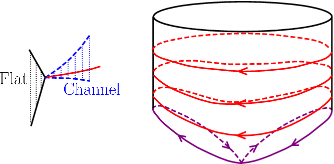
To be more precise, let us study this phenomenon in the finite covering space where for if we write for . Let : be a permutation such that the cardinality and . The lift of homoclinic curve as well as to contains several curves, not closed. Pick up one curve in the lift of , it determines a unique curve such that the end point of is the starting point of , and so on. See Figure 3.
We are going to show below that there exists a unique permutation such that one Aubry class in
as approaches to the vertex along the path in the channel. As the minimal curve is periodic with the homological class , the permutation : is -periodic. Since is prime to , we have if .
Lemma 3.4.
The permutation is uniquely determined by and . If , the following holds for
Proof.
By the assumption, there exists only one minimal homoclinic curve such that for . Because of the lemma 3.3, we can assume that and by choosing suitable coordinates on . We choose two sections and in a small neighborhood of the origin such that, emanating from the origin, these homoclinic curves pass through and successively before they return back to the origin as . In the section we choose disjoint subsections and such that the curve passes through for .
Let be the minimal periodic curve with rotation vector . For small , falls into a small neighborhood of these two homoclinic curves. So it has to pass either through or through . Let be the time for passing through with , and it does not tough these sections whenever . By definition, the period of the curve equals . If the curve intersects at and intersects at , then the segment keeps close to and keeps close to , so one has and .
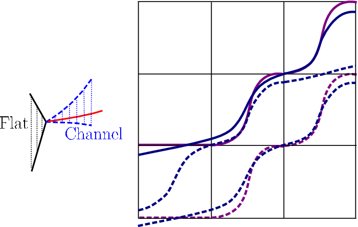
![[Uncaptioned image]](1207.4016v2/Ardiff4.png)
As the curve is minimal, it does not have self-intersection. Thus, once there exists such that and , then there does not exist such that and . Therefore, there is a set with cardinality such that for one has , for one either has and or has and .
By introducing coordinate transformation on : such that , let us think the curve as a straight line projected down to the unit square, a fundamental domain of . Starting from a point , the line successively reaches to the points where with small . To connect the point to the point , the curve does not touch the vertical boundary lines if
where denote the largest integer not bigger than the number , and it has to pass through the vertical lines at some point if
We define an order for these points such that iff and iff .
Returning back to the original coordinates, the curve falls into a neighborhood of the curves and , intersects the horizontal line at and intersects the vertical line at , and . Naturally, the map induces the order among these points: if and only if . If the curve passes the point at , the segment falls into a neighborhood of , otherwise, it falls into a neighborhood of . In this way, we obtained a unique permutation up to a translation.
![[Uncaptioned image]](1207.4016v2/Ardiff5.png)
∎
In the second case, some exists such that . It is typical that certain edge exists such that , the -minimal measure is supported on a hyperbolic periodic orbit for each . Thus, there is a channel endding at such that the family of periodic orbits constitutes a normally hyperbolic cylinder.

In the following, we shall study the dynamics on certain energy level of truncated normal form . Since one obtains the condition from the normal form, some function solves the equation . Treat as the new Hamiltonian and let be the time, one obtains a system with two degrees of freedom, which is equivalent to the dynamics on the energy level .
Theorem 3.4.
For the Hamiltonian we assume that on . Let be the solution of . Let and be the -function for and respectively, where
Then for we have .
Proof.
Let , , and . Let be -minimal curve for the Lagrange flow , is then -minimal curve for the Lagrange flow if and is re-parameterized . If is a solution of , one obtains from the Hamiltonian equations. Since , we find
This completes the proof. ∎
Let be the projection . By this theorem, is a homeomorphism for , the -neighborhood of the flat . Thus, what we obtained in this subsection have their counterpart in the energy level set where the class .
4. Normally hyperbolic invariant cylinder
In this section, normally hyperbolic invariant cylinder is proved to exist in certain neighborhood of double resonant point. It uses the normal form which is obtained in the appendix where several steps of KAM iteration and one step of linear coordinate transformation were carried out. All these coordinate transformations are symplectic. Since Aubry set and Mañé set are symplectic invariants [Be2], it is good enough to study these objects by considering the normal form.
4.1. Homogenized Hamiltonian
The normal form of the Hamiltonian takes the form
| (4.1) |
where and . Since is positive definite, a unique curve exists along which . This curve passes through the energy level transversally at a unique point . As , one has . By coordinate translation, we assume .
As the dynamics we are going to study is restricted on an energy level , it can be reduced to a system with two and half degrees of freedom. Since , the equation uniquely determines a smooth function in certain neighborhood of . Treating as a new Hamiltonian and as a new time variable, we obtain a time-periodic system with two degrees of freedom. Correspondingly, we have the normal form
| (4.2) |
where , and is as small as .
Each determines a resonant curve . Normally hyperbolic cylinder is searched when varies along this curve. Recall that the normal form remains valid in the domain (). The -neighborhood of the curve is covered by as many as small balls with radius . Given a ball centered at , by rescaling variables , , one obtains an equivalent Hamiltonian equation
which corresponds to the Hamiltonian
where , , and
According to Appendix A, one has and , where the -norm is with respect to only. To guarantee the covering property shown in the appendix, one choose , so we have . Obviously, one has
Proposition 4.1.
Each orbit of the Hamiltonian flow uniquely determines an orbit of . If and , then .
The Hamiltonian is a small perturbation of the homogenized Hamiltonian
which determines the Lagrangian
Let us first consider the case when , it follows that . The variable is restricted in the domain , where the higher order term is bounded by (see (A.1)). Correspondingly, let and for :
For this Hamiltonian system, the maximal point of determines a stationary solution which corresponds to a minimal measure of , where the matrix
has 4 real eigenvalue . By translation of coordinates, it is generic that
(H1): attains its maximum at only, the Hessian matrix of at is negative definite. All eigenvalues are different: .
Such a hypothesis leads to certain hyperbolicity of minimal homoclinic orbits. Let us consider the case: for the Aubry set , where : is a minimal homoclinic curve. By the assumption H1, the fixed point has its locally stable manifold as well as the locally unstable manifold . They intersect each other transversally at the origin. As each homoclinic orbit entirely stays in the stable as well as in the unstable manifolds, along such orbit their intersection can not be transversal in the standard definition, but transversal module the curve:
holds for is on minimal homoclinic curves. Without danger of confusion, we also call the intersection transversal.
If we denote by the eigenvector corresponding to the eigenvalue , where and are for the - and -coordinate respectively, then the eigenvector for will be . it is also a generic condition that
(H2): with each , there is at most one minimal orbit associated, the stable manifold intersects the unstable manifold transversally along each minimal homoclinic orbit. Each minimal homoclinic orbit approaches to the fixed point along the direction : as .
Recall the set . If , the -minimal measure consists of two or more ergodic components. Because of Theorem 3.3 and the countability of homology classes of all homoclinic curves, we have another generic condition
(H3): For each , the Aubry set does not contain minimal curve homoclinic to the origin fixed point.
4.2. Cylinder for truncated Hamiltonian: near double resonance
Let us start with a Hamiltonian with two and half degrees of freedom:
| (4.3) |
where , , (see Theorem A.1) where the -norm is with respect to . Recall the homogenized Hamiltonian as well as the homogenized Lagrangian
where .
By the assumption (H1), the fixed point each which is a 2-dimensional flat. As classified before, for each the Aubry set consists of minimal homoclinic orbits plus the fixed point.
Given an irreducible class , it is not necessary that some minimal homoclinic curve exists such that . Let us consider the -minimal measure for with . As we shall see later, it is generic that the minimal measure is supported on at most two periodic orbits, denoted by , both are hyperbolic, namely, it has the stable and unstable manifold. These periodic orbits constitute a two-dimensional cylinder. However, it appears not reasonable to assume the normal hyperbolicity for in usual sense as the speed along the orbit may undergo large variation, especially, when it is very close to some homoclinic orbit. Therefore, one can not see the separation of the spectrum of in normal and in tangent direction. As the first step, let us study the case when .
There are two cases alternatively as decreases: as decrease to zero, or such that .
In the first case, the cohomology class approaches to some edge or to some vertex where two adjacent edges joint together. Under the hypothesis (H2), for class in the interior of the edge, the Aubry set contains exactly one minimal homoclinic curve and the point of the origin. Let be the minimal homoclinic curve related to for , it determines the minimal homoclinic orbit . Denote by the homology class. If , as decreases to zero. If there exist two positive integers such that , the curve approaches to the set (figure eight) as , folding and -times along and respectively.
The periodic curve determines a periodic orbit in the phase space. It stays in certain energy level set . For and suitably small , by the study in Section 3.2 (Eq.(3.12)), the period is related to the energy by the formula
where as , both and is bounded.
To study the dynamics around the minimal homoclinic orbits (), we use a new canonical coordinates such that, restricted in a small neighborhood of , one has the form
where . Without losing generality, we assume as , as and as . Here the notation is taken as granted: . We choose 2-dimensional disk lying in
Because of the special form of , one has
Let () denote the unstable (stable) manifold of the fixed point which entirely stays in the energy level set . If , the tangent vector of has the form . So, the tangent vector of takes the form
where both and are small.
Denote by the time when the homoclinic orbit passes through . As holds at the point , both homoclinic orbits and approach in the same direction to the fixed point, the section as well as intersects these two homoclinic orbits transversally. Let denote the intersection point of with . In a small neighborhood of that point , one obtains a map : in following way, starting from a point in this neighborhood, there is a unique orbit which moves along and comes to a point after a time approximately equal to .
Let us fix small . There exists (depending on ) such that
holds for both and . Clearly, one has as .
As the homoclinic curves approach to the origin in the direction of in -space, for small , there exists a constant such that as and
The Hamiltonian flow defines a map : and a map : : emanating from a point in () there exists a unique orbit which arrives () after a time bounded by the last formula.
Restricted in the ball , let us consider the variational equation of the flow along the homoclinic orbit . It follows from the normal form of the homogenized Hamiltonian that the tangent vector satisfies the variational equation
| (4.4) |
where . Clearly, with if is small. Since the homoclinic orbit approaches to the fixed point in the direction of , one has
For the initial value satisfying the condition
one obtains from the hyperbolicity that
holds for some constant depending on as well as on . Therefore, for each vector which is nearly parallel to : holds for we obtain from the last two formulae that
Similarly, one has
where also depends on as well as on , and as .
By the construction, the 2-dimensional disk intersects the unstable manifold along a curve. Let be a very short segment of the curve, passing through the point . Pick up a point on the homoclinic orbit far away from the fixed point and take a 2-dimensional disk containing the point and transversal to the flow in the sense that . The Hamiltonian flow sends each point of to this disk provided it is close to . In this way, one obtains a map : . Let . According to the assumption (H2), one has . Thus, one also has . It follows from the -lemma that keeps -close to at the point and keeps -close to at the point provided is sufficiently small. As , one obtains
and
where . See the figure below.
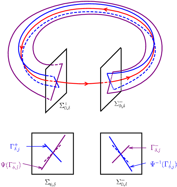
Recall the definition, is a two-dimensional disk lying in the energy level set . For sufficiently small, is -close to respectively. Let be the minimal periodic orbit staying in the energy level set , it approaches to the homoclinic orbit as decreases to zero. Thus, for sufficiently small , it passes through the section as well as times for one period. We number these points as () by the role that emanating from a point , the orbit reaches to the point after time , then to the point and so on. Note that remains bounded uniformly for any . Restricted on small neighborhoods of these points, denoted by , the flow defines a local diffeomorphism : . Because of the smooth dependence of ODE solutions on initial data, a small exists such that, for the vector -parallel to in the sense that holds for some , we obtain from the hyperbolicity of (see the formulae above Figure 5) that
and
where , as . If the vector is chosen -parallel to then the vector is -parallel to .
For , the Hamiltonian flow defines local diffeomorphism : . To make one has as . According to the study in Section 3.2 (cf. formula (3.12)), starting from , the periodic orbit comes to after a time approximately equal to
in which is uniformly bounded as . Given a vector , we use denote the -component. For a vector -parallel to , there is such that . From Eq.(4.3) one obtains
| (4.5) | ||||
where as . It follows that the vector is -parallel to and
where and as . Similarly, for a vector -parallel to , one sees that the vector is -parallel to and
The composition of the two maps constitutes a Poinćare map , it maps a small neighborhood of the point in to a small neighborhood of the point in . For a vector -parallel to the vector is still -parallel to
| (4.6) |
and for a vector -parallel to the vector is still -parallel to
| (4.7) |
holds for each , where , as . Therefore, each point is a hyperbolic fixed point for the map , is a hyperbolic orbit of . By Lemma 3.4, these points are uniquely ordered, is the minimal period. As these points approach to the fixed point as , the hyperbolicity guarantees the uniqueness. It also guarantees the smooth continuation of periodic orbits. Therefore, we have
Lemma 4.1.
Assume the conditions (H1) and (H2) and let be a class. If as , then there exists such that for each with the Mather set consists of exactly one periodic orbit.
Let be a two-dimensional disk transversally intersecting the orbit at such that for and let : be the return map naturally determined by the flow , there exists some independent of such that
where is the point where the periodic orbit intersects , denotes the stable unstable manifold of the periodic orbit. Therefore, the periodic orbits for constitute a smooth cylinder.
In the second case, some exists such that . It is typical that is an edge of , where each Mather set consists of a hyperbolic periodic orbit and the fixed point. The uniqueness of minimal periodic orbit for close to follows from the implicit function theorem.
Given , the set is a channel in . There is a path reaching to the boundary , along which the -function monotonely decreases to the minimum as the cohomology class approaches to . With the argument as above and Theorem B.2 shown in the appendix, we find the following condition also generic
(H4): Given a class and an energy , there are at most finitely many such that for with the Mather set consists of two periodic orbits, for all other with , the Mather set consists of exactly one periodic orbit. All these periodic orbits are hyperbolic.
We call these bifurcation points. Let be the smallest one. Each energy uniquely determines a hyperbolic periodic orbit . Thus, we introduce a notation
with small . It is a two-dimensional cylinder composed of a family of periodic orbits, may approach to a curve of figure-of-eight as decreases to zero. Obviously, the cylinder is invariant for the Hamiltonian flow of . Let denote the period of the periodic orbit in , one has
The cylinder may be slant and crumpled, not standard. To see how the symplectic area is related to the usual area of the cylinder, let us study the dependence of the fixed point of the Poincaré return map on . By definition, the fixed point is a solution of the equation
| (4.8) |
Emanating from a point the orbit reach a point after a time which remains bounded as . Let be the point corresponding to , obtained in the same way. The difference of the -coordinate of these two points is bounded by where depends on . Let be the solution of the variational equation (4.3) along the periodic solution passing through a neighborhood of the origin, let be the time such that the first coordinate and , the quantity is bounded by (3.12). In virtue of the formula (4.5), it yields
where as . Therefore, we find that
As the quantity is bounded by (4.6), the quantity for the inverse of is bounded by (4.7), we obtain from the equation (4.8) that
| (4.9) |
It yields a relation between the symplectic area and the usual area of the cylinder
| (4.10) |
Theorem 4.1.
We assume the conditions (H1, H2, H4). For each , the cylinder is normally hyperbolic for the map , where .
Proof.
For any , the cylinder is a 2-dimensional symplectic sub-manifold, invariant for the Hamiltonian flow . However, it is not clear whether this cylinder is normally hyperbolic for the time-1-map , as it is possible that
and we do not have the estimate on the norm of acting on the normal bundle.
As the first step of the proof, let us search for the normal hyperbolicity of with large for the cylinder , where denotes the largest value such that the formulae (4.6) and (4.7) hold for each . From these formulae, one sees that the smaller the energy reaches, the stronger hyperbolicity the map obtains. The strong hyperbolicity is obtained by passing through small neighborhood of the fixed point. However, on the other hand, the smaller the energy decreases, the longer the return time becomes.
Let denote the time interval such that, starting from , the periodic orbit comes to after time . In virtue of the study in Section 3, Eq. (3.12),
where is uniformly bounded and we take if the segment of the periodic orbit keeps close to the homoclinic orbit . Note is much larger than . Thus, starting from any point on the minimal periodic orbit , passes through the neighborhood of the fixed point after time . It implies that the map obtains strong hyperbolicity on normal bundle.
To measure how the map acts on the tangent bundle, let us study how the map elongates or shortens small arc of the periodic orbit. As the orbit passes through the neighborhood of the origin in a time approximately equal to the variation of the length of short arc is between and , where is small. Because of the relation between the symplectic area and the usual area of the cylinder, given by the formula (4.10), the variation of , restricted on the tangent bundle of the cylinder, is between and . Because of periodicity, it is independent of .
Thus, the normally hyperbolic property becomes clear: the tangent bundle of over admits -invariant splitting
and some , and small exist such that
| (4.11) |
hold for (cf. (4.6) and (4.7)). Note that provided is suitably small. The formula (4.11) satisfies the definition of normal hyperbolicity.
For each , let be the minimal periodic orbit, be a 2-dimensional disk intersecting transversally at the point , : be the Poincaré return map. By the generic property (H4), is the hyperbolic fixed point of and exists such that
As the cylinder is foliated into periodic orbits and preserves the symplectic form, some exists such that
holds for any . Choosing such that , one obtains the normal hyperbolicity for with , where is the period of the periodic solution in , with . By choosing suitably small , we have . ∎
4.3. Persistence of cylinder: near double resonance
To apply the theorem of normally hyperbolic manifold [HPS] to the Hamiltonian of (4.3), we note that the Hamiltonian is autonomous with two degrees of freedom. As , and because of the non-degeneracy assumption for ((H1,H2)), we see that for each suitably small , the map admits invariant cylinder also, denoted by still, with the normally hyperbolic properties (see Formulae (4.11)), independent of the size of .
Let us consider the persistence of with with . As the perturbation depends on time , we use to denote the map from the time -section to the time -section, omit the symbol if . Since these hyperbolic properties are posed for the map with large , one has to measure how large the quantity will be. As is autonomous, .
Lemma 4.2.
Let the equation be a small perturbation of , let and denote the flow determined by these two equations respectively. Then
where and .
Proof.
Let denote the solution of the equations for respectively, and . Let , then and
where . Therefore, one has
Let , we have . It follows from Gronwell’s inequality that
Along the orbit , the differential of the flow obviously satisfies the equation
Therefore, for each tangent vector attached to one has
To study the differential of , let us consider the equation of secondary variation. Let be the solution of the variational equation for respectively, where solves the equation and . To measure the size with the condition , we make use of the relations such as , and find that
Let , we have . Using Gronwell’s inequality again, one obtains an upper bound of the variation of the differential
Note that represents initial tangent vector, it completes the proof. ∎
Let us applying this lemma to the Hamiltonian . Treating as the function of we find that there exist some constants independent of such that
as (see Theorem A.1). Since the function comes from which is -smooth (), one has . For one obtains from Lemma 4.2 that
If the condition is satisfied, then as . It allows one to apply the theorem of normally hyperbolic manifold to obtain the existence of invariant cylinder for the flow in the extended phase space , which is a small deformation of .
Be aware of the fact that is a cylinder with boundary, normally hyperbolic and invariant for , where , we do not expect that the whole cylinder survives small perturbation, it may lose some part close to the boundary. To measure to what range the cylinder survives, we see that the variation of the energy along each orbit of is bounded by
| (4.12) |
here, the estimate is used (see Theorem A.1). Assume that the number satisfies the condition
| (4.13) |
one sees that, starting from the energy level , after a time of , the orbit of can not reach the energy level if is suitably small so that . Indeed, under such condition one has
| (4.14) | ||||
To use the theorem of normally hyperbolic invariant manifold, let us introduce a modified Hamiltonian. Let : be a smooth function so that for and for ,
it coincides with for with and coincides with for with . For small satisfying the condition (4.13) and small , the cylinder survives the perturbation and the bottom remains invariant for .
By the definition, one has for with and it follows from (4.14) that provided and . So, for the invariant cylinder persists under the perturbation , denoted by . A point implies . The invariance is in the sense that, emanating from any point in , the orbit has to pass through the bottom of the cylinder if it is going to leave the cylinder.
Location of Aubry set in the cylinder
As the working space here is phase space, we say that an Aubry set is located in the cylinder if for each -static curve , the orbit in the phase space .
Recall the Hamiltonian defined in (4.3) and note the Hamiltonian is autonomous. Let and denote the -function for the Lagrangians determined by and respectively.
Since is a hyperbolic cylinder, invariant for the Hamiltonian flow , the channel has a foliation into a family of segments of line (one-dimensional flat), where is chosen so that for each if . We claim that the -function is smooth in . Indeed, restricted on each of these flats the function keeps constant, while restricted on a line orthogonal to these flats, the function is smooth because can be treated as a Hamiltonian with one degree of freedom when it is restricted on the cylinder. If we consider the Hamiltonian in the finite covering space where for if we write for . In that space there are fixed points. Because of Hartman’s theorem for two-dimensional system, it is -conjugate to a linear equation , around each fixed point. Therefore, for small some -function exists such that the period of the frequency is (see (3.12)). Since
| (4.15) |
As remains constant when it is restricted on each of its flats which are orthogonal to the line , we find that for
| (4.16) |
where is the direction of and . It follows that
| (4.17) |
holds for , , .
Let be the class so that . To measure the difference of , we find . As the -function undergoes small variation: for small perturbation with [Ch], we find when is restricted on the path . Therefore, we obtain that
| (4.18) |
Lemma 4.3.
In the Aubry set for with , any orbit does not hit the energy level set with .
Proof.
If the lemma does not hold, there would exist an orbit in the Aubry set for , which hits the energy level at the time , i.e. . Since the orbit entirely stays in the invariant cylinder and the perturbation is of order , it returns back to the neighborhood of after a time where remains bounded as . To see how close it could be, we obtain from (4.12) that
| (4.19) | ||||
As is an invariant circle for , the perturbed cylinder is -close to the original one [BLZ] and the cylinder may be crumpled but at most up to the order (cf. (4.9)), some large exists such that and
Since the curve is assumed -static, it follows that
| (4.20) |
As the cylinder is -close to , there is a -minimal orbit of the Hamiltonian flow on such that and . Let and where is the period of , we have an estimate on the Hausdorff distance . Consequently, we have
As we have
Let be the lift of to the universal covering space, it follows that
Since it follows from (4.19) that
holds for all , we find
| (4.21) | ||||
To verify the second inequality, let be the class such that , then we obtain from the formula (4.18) that
For small such that we find from (4.15) that
holds for and . Therefore, one obtains from (4.16) and (4.17) that
from which one obtains the second inequality of (4.21) from the first one. As is very small, the formula (4.21) contradicts (4.20). It completes the proof. ∎
For satisfying the condition (4.13), going back to the original coordinates (, and ), we obtain
Theorem 4.2.
For an irreducible class , there exists a 3-dimensional cylinder associated with a channel such that
1, the cylinder is a small deformation of the cylinder
where , is the minimal periodic curve for , the function solves the equation , and ;
2, the cylinder is invariant for the Hamiltonian flow : , if holds for then such that is on the boundary of , where solves the equation ;
3, is normally hyperbolic for with ;
4, this channel reaches to a small neighborhood of the flat in the sense
For each with , the Aubry set entirely stays in the cylinder.
Let us consider the autonomous Hamiltonian with the form of (4.1). Let , be the function solves the equation . Then has the form of (4.2). The energy of corresponds to the coordinate for the autonomous Hamiltonian . Applying Theorem 3.4 one obtains
Theorem 4.3.
Assume . Given an irreducible , there is a -dimensional cylinder associated with a channel such that
1, the cylinder is a small deformation of the cylinder
2, the cylinder is invariant for the Hamiltonian flow : for each , if holds for certain then such that is on the boundary of ;
3, is normally hyperbolic for with ;
4, for each with , the Aubry set is contained in that cylinder .
By H4, it is generic that there are finitely many bifurcation points, denoted by corresponding to the energy . For each point , the -minimal measure for the Hamiltonian is uniquely supported on a hyperbolic periodic orbit. For the class , the Mather set is composed of two hyperbolic periodic orbits. The periodic orbits for constitute a piece of cylinder . As these periodic orbits are hyperbolic, the cylinder can be extended a little bit consisting of periodic orbits which are hyperbolic also, but do not support minimal measure. They are local minimal. These cylinders are clearly invariant and normally hyperbolic for the Hamiltonian flow with suitably large . Applying the theorem of normally hyperbolic manifold, one can see that there exists some which is invariant for the Hamiltonian flow determined by , and keeps close to . For each , the Mather set for stays in the cylinder. Except for finitely many very close to , the time--section of the Mather set for other is an invariant circle, or periodic points or Aubry-Mather set in the cylinder, for bifurcation point , the Mather set consists of two parts, one stays in another one stays in .
4.4. Transition from double to single resonance
Some normally hyperbolic invariant cylinder has been shown to reach -neighborhood of the double resonant point. This cylinder extends to the place a bit far away from the double resonant point. To see how to transit from double resonance to single resonance, let us homogenize the Hamiltonian in a region and choose different . Recall that the normal form remains valid in the domain (). The -neighborhood of the curve is covered by as many as small balls with radius . Such approach is based on the following:
Proposition 4.2.
For nearly integrable Lagrangian , each orbit in Mather set
The result is proved in [BK] for time-1-map. It is also true for the Hamiltonian flow i.e. . It makes sense for us to homogenize the Hamiltonian in the range with suitably large .
Using new variables and , the homogenized Hamiltonian equation turns out to be the following form
where , the frequency satisfies a resonant condition. The corresponding Lagrangian reads
With the potential on the torus one associates its time average along the orbits of the linear flow defined by :
where is the period of the frequency . The function is then defined on a circle. Let be the maximal point of , it corresponds to a circle on . The averaged Hamiltonian is also associated with a Lagrangian
Let be the period of the frequency , : be the minimizer of the action
then it is a curve of maximal points of with constant speed . Consider as a function defined on and denote by the second derivative for the variable of , where we use to denote the circle .
Let denote a translation of such that and let : be the minimizer of the action
then we have
Proposition 4.3.
Assume is non-degenerate at its minimal point , and assume some exists so that . Then there exist some constants such that the minimizer entirely stays in -neighborhood of the circle , i.e. holds for each and .
Proof.
Since the minimizer solves the Lagrange equation, its second derivative remains bounded. Thus, as the first step, we claim that the minimizer stays entirely in -neighborhood of , a translation of the circle . If not, the oscillation of in the direction perpendicular to would not be smaller than . As the average speed is , there would be a point on the minimizer where . Since the potential is bounded , one obtains that if we choose . On the other hand, the action along the curve would be not bigger then . The contradiction implies our claim.
Let us compare the action of along the curve with that along the curve . If , by what we have proved, some exists such that
It follows that
it contradicts the minimality of the curve if is chosen suitably large. ∎
Recall the picture of minimal periodic orbit close to double resonance, one can see from this proposition how the shape of the periodic orbit changes when it moves away from double resonance to single resonance.
5. Annulus of incomplete intersection
Let us also start with the Hamiltonian defined by Formula (4.3), it has two and half degrees of freedom. Given any two homology class , The theorem 4.2 confirms the existence of two wedge-shaped regions and which reach to the boundary of the annulus
For each class in and , the Aubry set lies in the normally hyperbolic cylinder and, by the result for a priori unstable systems, can be connected to other Aubry set lying in the cylinder under certain generic conditions. However, it seems unclear whether these two wedges can reach to the flat . Thus, a notable difficulty rises as these cylinders are separated by an annulus around the flat , it is the problem of crossing double resonance.
It is the goal of this section to find an annulus where those two wedge-shaped regions are plugged into and for each class in that annulus, the stable set of the Aubry set “intersects” the unstable set non-trivially, possibly incomplete. In other words, for each class in this region, the Mañé set does not cover the whole configuration space.
5.1. The Mañé set for
As the first step, let us consider the Hamiltonian and study all cases when the Mañé set covers the whole configuration space.
For each , except for the minimal measure supported on the fixed point , some minimal measure exists with non-zero rotation vector. In the covering space : , a disk is contained in a strip bounded by two -static curves and , both curves are in the Mather set: no other -static curve in the Mather set touches the interior of this strip. Let and denote the elementary weak KAM solution determined by and respectively, we investigate what happens when holds in this strip. As the configuration space is two dimensional, for each in this region, uniquely determines a -semi static curve which lies entirely in this strip. The -semi static curves considered here are all determined by . It is possible that some curve approaches to the origin as , in this case, because of H3, it approaches to the curve () as ().
Supported on the fixed point, the measure is minimal for all . Thus, there always exists some semi-static curve connecting the fixed point to the support of other -minimal measure
As all eigenvalues are assumed different, generically, all minimal homoclinic curves approach to the fixed point in the direction , associated to the smallest eigenvalue:
But this does not exclude the possibility that some -semi static curves approach to the point in the direction of . It provides us a criterion to classify the cases when the Mañé set covers the whole configuration manifold.
Case 1: no -semi static curve approaches the origin in the direction of . In this case, as , there exist exactly two semi-static curves such that as . They approach the origin in the direction and
Other cases are classified under the condition that there exist some -static curves approaching the origin in the direction of . Since the curves as well as is disjoint with the origin, some number exists such that these two curves do not hit the ball . The number seems depending on . Let be a semi-static curve approaching the origin as , it intersects the circle at some point. Let be such a set that passing through each point a -semi static curve approaches to the origin, as , in the direction of . By assumption, the set is not empty. Obviously, does not occupy the whole circle and can be made closed by adding at most two points, through which some semi-static curves approach the origin in the direction of .
Passing through a point very close to , there is a unique -semi static curve, determined by . Because of Proposition 3.2, the curve will get very close to the origin and leave in a direction far away from . Let be a connected component of , it may be a point or an interval. If it is a point, let be two sequences of points such that they approach from different sides. Let () be the semi static curve passing through (), it shall intersect the circle at a point () respectively. Some exist so that , as .
If , it determines a -semi static curve approaches the origin as . Because of Proposition 3.2, it approaches in the direction of . This leads to
Case 2: there exists exactly one -semi static curve approaching origin in the direction of .
If , let denote the arc bounded by these two points, not containing . One can see from the proof of Proposition 3.2 that the angle of this arc is not smaller than . Passing from each point in the interior of the arc, the -semi static curve approaches to the origin as and these curves constitute a sector. Since the fixed point is hyperbolic, it has its stable and unstable manifolds . Thus, some some generating function and exist such that . As the orbits determined by the curves entirely lie in the unstable manifold of the fixed point, one has in the sector. Therefore, the size of the sector-shaped region is independent of the size of . This leads to
Case 3: in the disk there is a sector-shaped region with the field angle not smaller than . In this sector, one has .
Let () be -semi static curve passing through a point in () respectively, then they approach the origin in opposite direction as respectively, i.e. . To verify this claim, let us assume the contrary. Thus, these two curves cut the ball into two parts, one is sharp wedge-shaped, denoted by .
![[Uncaptioned image]](1207.4016v2/Ardiff8.png)
We choose a -semi static curve lying in and keeping very close to the curves and . In canonical coordinates such that , the set has a vertex at the origin. As both and approach the origin in the direction of , there exists such that if and . Since the fixed point is hyperbolic, it has local stable and unstable manifold, determined by the generating functions and respectively. Restricted in , these functions satisfy the condition
Pick up two points and very close to respectively, through which some -semi static curve passes, namely, some exist such that and . Note the orbit determined by () lies in the stable (unstable) manifold, by definition ones has
If we choose sharing the same first coordinate with and connect them with a straight line : , then and the action along this curve one has . It contradicts the minimality of , thus the claim is proved.
We claim that has only one connected component. Otherwise, there would be two connected component and . By the definition, passing through a point () there is a -semi static curve () which approaches the curve as and approaches the origin as . These two curves divided the strip into two parts , where is such a strip that passing through any point , the -semi static curve will approach the origin as . However, there exists a point , it implies that passing thorough , the -semi-static curve will approach the curve , namely, it would intersect either or . It is absurd. Thus, we obtain the left picture in Figure 6.

By similar argument applying to the set , we have either the case 2 again or
Case 4: in the disk there is a sector-shaped region with the field angle not smaller than , where , see the right picture in Figure 6.
We claim that all of these cases do not occur for generic potential . The first two cases takes place at most for four invariant measures, as there are only four curves which approaches the origin in the direction of . Each of these curves approaches at most one Mather set. These Mather sets correspond to at most four edges of . Let be a non-negative function such that its support does not touch these four curves as well as the support of the minimal measure. By perturbing the potential , one can see that the Mather set remains unchanged, but the Mañé set does not cover for each of these four cohomology classes.
Both case 3 and 4 take place also for at most four Mather sets, as each sector-shaped region has the field angle not smaller than , and the orbit determined by approaches one Mather set only. Let us destruct it one by one. If some sector-shaped region exists where , . We divide it into three sub-sectors , each of which is composed of -semi static curves approaching the origin as and is disjoint with . We introduce another potential such that the function is non-negative, ().
For the perturbed Lagrangian determined by , the minimal measure for the class is the same as that for unperturbed Hamiltonian. Let , be the elementary weak KAM solutions of the perturbed Hamiltonian, associated to the minimal measure and respectively, one has
Under such perturbation, there might be another cohomology class such that holds on the whole torus and a sector exists where . Note , we split it into three sub-sectors , each of which is composed by -semi static curves approaching to the origin as and is disjoint with . We introduce again a perturbed potential such that the function is non-negative, ().
For the new perturbed Lagrangian, the minimal measure for the class is the same as that for unperturbed one. Let , be the elementary weak KAM solutions of the perturbed Hamiltonian, determined by and respectively, one also has
For suitably small , the Hamiltonian flow determined by is well approximated by its linearized flow when they are restricted in the ball . For the linearized flow, if is an orbit in the unstable manifold, is an orbit in the stable manifold. Therefore, some sectors () exist so that , and hold for , each consists of -semi static curves which approach the origin as with
each consists of -semi static curves which approach the origin as and
Since there are at most two sectors corresponding to unstable manifold and two sectors corresponding to stable manifold, there are at most four pairs of static curves () for which the case 3 and 4 takes place.
These four pairs of static curves () corresponds to four edges (points) contained in . By construction, the Mañé set does not cover the whole torus for each cohomology class one these four edges. For any other class , the Mañé set can not cover the whole torus also. Otherwise, there would be a sector of where , but it is absurd since some where holds for some . For each , determines an orbit of the Lagrangian flow which approaches both to the support of and to the support of as , it is impossible. Therefore, we have
Lemma 5.1.
It is an open and dense condition for the potential that for all class , the Mañé set does not cover the torus: .
5.2. The Mañé set for
This set contains at most countably many vertexes. Indeed, if both and are non-empty, there do exist countably many vertexes (cf. Theorem 3.3).
Let be an edge joined to other two edges at the vertex , respectively. By Theorem 3.3, the Aubry set for consists of two minimal homoclinic curves and . Denote by the homology class of , then the matrix is uni-module. By introducing suitable coordinates on , we can assume . In this coordinate system, and .

In this figure, each unit square represents a fundamental domain of in the universal covering space, the horizontal line represents the lift of the homoclinic curve , which stays in the Aubry set for each . The blue dashed lines represent the lift of the which stays in the Abury set for the class at one end-point of . The purple dashed lines represents the lift of the which stays in the Abury set for the class at another end-point of .
Let us consider weak KAM solution in the strip bounded by the lines and . According to Lemma 4.1, for very small, there exists an interval such that for each , the Mather set consists of only one closed curve such that . In the universal covering space, let be a component of the lift of which approaches as . Let be the elementary weak KAM solution determined by . As , in -topology. The function is obtained in the same way. The function determines backward semi-static curves approaching to the line as the time approaches to minus infinity, determines forward semi-static curves approaching to the line as the time approaches to positive infinity respectively.
If we remove the coercive condition on these weak KAM solutions that determines a backward (forward) semi-static curve approaching (), then the weak KAM depends on (no longer elementary). As for each , starting from a point close to the line (), the backward (forward) semi-static curve will approach to ().
Let . For each , by Proposition 2.3, the strip is divided into two connected parts and such that and . Let be the forward semi-static curve determined by , starting from the point . If , the curve is calibrated for which induces
| (5.1) | ||||
where both and exist. Note where is the standard projection. One can see from Figure 7 that
It follows that the inequality (5.1) also holds for , which implies that also. Clearly, expands and shrinks as increases. As the limit, we see that and occupies the whole strip. Therefore, we have:
Proposition 5.1.
Assume be an edge joined to other two edges at the vertex , respectively. Let be the globally elementary weak KAM for with . Then, for each , the weak KAM solution is completely determined by and in the following sense: there is a partition such that is connected,
where and if , and .
In virtue of this proposition, we see that, for all , the set of barrier functions are determined by countably many weak KAM solutions. For each edge , there is an open-dense set in space such that holds for each if the potential takes value in this set. Therefore, in virtue of the lemma 5.1, we have
Theorem 5.1.
Let . A residual set exists such that for each and for each , the Mañé set does not cover the whole configuration space: .
Because of this theorem, we have generic hypothesis
(H5): The potential is chosen so that the Mañé set does not cover the whole torus for each .
5.3. Thickness of the annulus
The Hamiltonian under consideration is given by the formula (4.1) which is autonomous. To start with, let us assume assume and study elementary weak KAM solutions of the Hamilton-Jacobi equation
| (5.2) |
where solves the equation and . Expanding the Hamiltonian into Taylor series of , replacing by and rescaling by we obtain the equation
| (5.3) |
where is the Hessian matrix of in at , (cf. formula (4.3)). In this equation, only higher order term depends on the time . As the first step to study the weak KAM of this Hamilton-Jacobi equation, we omit the higher order term and let . Since the potential is independent of the time , all elementary weak KAM solutions discussed in the last two subsections solve the equation
| (5.4) |
and for each and each , the weak KAM solutions of this equation define a Mañé set which does not cover the whole torus: . By the upper semi-continuity of the set of semi-static curves, some small exists such that for each positive and each (We use to denote the -function determined by the Hamiltonian ) the Mañé set does not cover the torus. It implies that holds if , both and are the weak KAM solutions of the equation 5.4 with .
For each average action , the dynamics on the energy level is similar to twist and area-preserving maps. First of all, the rotation vector of each minimal measure is not zero. Thus, any minimal measure is not supported on fixed points. Secondly, for each class , all -minimal measures share the same rotation rotation direction, otherwise, the Lipschitz graph property will be violated. If the rotation direction is rational, each ergoidc minimal measure is supported on a periodic orbit.
From these properties one derives the following: for each , there exists a circle such that each semi-static curve passes through it transversally and . Since the set is closed, there exist finitely many intervals disjoint to each other such that .
As these functions are independent of , all of these functions can be thought as the weak KAM solutions of the homogenized Hamilton-Jacobi equation
if they are thought as the function of the variable . Here, the cohomology class takes value on the circle: . It follows that, for each class , there exists non-degenerate embedded two-torus and finitely many intervals disjoint to each other such that each -semi-static curve passes through the two-torus transversally and . Here the circle is for the time .
Let us return back to the Hamilton-Jacobi equation (5.3). Recall the normal form of the Hamiltonian, we see that in the remainder , one contribution is from (see the formula (4.3)), other contributions are independent of . Again, by the upper semi-continuity of the set of semi-static curves, we have
Theorem 5.2.
Under the hypotheses H1H3, H5, some positive numbers and exist, depending on the potential , such that for each , each and each , all semi-static curves pass through transversally the two-torus ,
| (5.5) |
where is a circle located in a 2-torus , are closed intervals, disjoint to each other and independent of the time .
Here, the semi-static curves are in the sense of extended configuration space, i.e. if is a curve, we also call its graph a curve .
Let us go back to the original scale. By Theorem 5.2, there exist a annulus-shaped region
such that the condition (5.5) holds for each . Recall this time-periodic system is deduced from the autonomous system restricted on certain energy level . In virtue of Theorem 3.4, the counterpart of in is
where we notice that the sphere is located in the upper half space of and touches the plane where .
In the original coordinates , Theorem 5.2 states such a fact: for each , all -semi static curves pass through the 2-torus transversally and all intersection points are restricted in the strips . However, the condition (5.5) dost not guarantee complete “intersection” of the stable set with unstable set, in the sense that the set contains some disconnected points. Therefore, we call the annulus of incomplete intersection. In this case, we do not expect to construct orbits connecting each Aubry set to any other Aubry set nearby, possible incompleteness may block some direction. However, once non-trivial intersection exists, it opens way to connect some Aubry set nearby. We shall show it in the subsection 7.2.
As provided is sufficiently small and , we obtain the following:
Overlap Property: Given any two irreducible , there exists a positive number such that the wedge-shaped regions intersects the annulus-shaped region: and provided .
6. Local connecting orbits
To construct orbits connecting some Aubry set to another one nearby, we introduce two types of modified Tonelli Lagrangian, namely, the time-step and the space-step Lagrangian. They satisfy the conditions of positive definiteness, super-linear growth and completeness. The time-step Lagrangian is not periodic in on the whole , instead, it is periodic when it is restricted either on or on , i.e. if or . The second type of Lagrangian is defined on some covering space. Let . The space-step Lagrangian is not periodic in one component of spaces coordinates . It is periodic in when it is restricted either on or on , i.e. if or .
The existence of local connecting orbits is established based on some upper semi-continuity of minimal curves for the modified Lagrangian.
6.1. Upper semi-continuity of minimal curves
Time-step Lagrangian: Let us consider time-step Lagrangian first. A curve is called minimal if
holds for any and for any absolutely continuous curve with and . Let denote the set of minimal curves for . Let , where is the standard projection.
Theorem 6.1.
The set-valued map is upper semi-continuous. Consequently, the map is also upper semi-continuous.
Proof.
Let be the diameter of the closed manifold , namely,
where denotes the length of the shortest geodesic connecting with . Let
As is assumed periodic for as well as for , is finite.
Let be a shortest geodesic connecting the point to the point . Given time interval with , we re-parameterize the geodesic by , then : is -curve such that , . Clearly, the action along this curve is not bigger than . Obviously, there is an upper bound uniformly for all minimizing action of if it is close to on , still denoted by
If the Lagrangian has super-linear growth, some positive numbers exist such that for all and for all close to . Therefore, if is a minimizer, one obtains
| (6.1) |
As (6.1) holds for any , it implies that there must be some for each such that . As it holds for any , therefore, some positive number exists such that
holds for all and for all relevant . It implies that holds for all .
Let be a sequence converging to in the following sense: there exists some , as well as a sequence of as such that . Let : be the minimizer of with , we then have for all . The set is compact in the -topology. Indeed, since is positive definite one can write the Lagrange equations in the form of , which implies is bounded in -topology.
Let : be one of the accumulation points of this set. Clearly, : is the minimizer of . Let and let and , we obtain a sequence of minimizers of , : . By diagonal extraction argument some subsequence of which converges -uniformly on each compact set to a -curve : . Obviously, it is a minimal curve of . This proves the upper semi-continuity. ∎
In application, the set seems too big for the construction of connecting orbits. For time-periodic Lagrangian, Mañé set can be a proper subset of , . It is closely related to the problem whether the Lax-Oleinik semi-group converges or not (cf. [FM]). For time-step Lagrangian, pseudo connecting curve is introduced to play roles similar to what semi-static curve does.
Each time-step Lagrangian uniquely determines two time-periodic Lagrangian and such that and . Let denote the minimal average action of . For and , we define
Clearly the limit infimum is bounded
Let and be the sequence of positive integers such that () as and the following limit exists
Let : be a minimizer connecting and
From the proof of Theorem 6.1 one can see that for any compact interval there is some such that the set is pre-compact in .
Lemma 6.1.
Let : be an accumulation point of . Then for
| (6.2) | ||||
Proof.
: To prove the lemma let us suppose the contrary. Thus there would exist , , , and a curve : with , such that
Let . By the definition of limit infimum there exist and such that
and there exist subsequences (; ) such that , and
holds for each . Let be the minimizer of . By taking a subsequence further one can assume . In this case, for sufficiently large , we are able to construct a curve : which has the same endpoints as : , and satisfies the following
Extending from to the by
and defining , we find that
But this contradicts the definition of the limit infimum as and . ∎
We define so-called pseudo connecting curve set
In application, we usually choose time-step Lagrangian so that the Aubry set of is different from that of . Clearly, for , the orbit approaches the Aubry set as and approaches as . That is why we call it pseudo connecting curve. Let
Clearly, if is periodic in , then and .
Theorem 6.2.
The map is upper semi-continuous. As the special case, the map as well as the map is upper semi-continuous.
Proof.
: Let be a sequence of time-step Lagrangian, let and let be an accumulation point of the set . We claim that . If , there would be two point , connected by another curve : and such that
where , . Since is an accumulation point of , for any small , there would be sufficiently large such that , and above inequality also holds for . It follows that , contradicting to the assumption. ∎
Space-step Lagrangian: Let and , where is for the coordinate . The space-step Lagrangian is introduced to handle the problem of incomplete intersection. A space-step Lagrangian also uniquely determines two Lagrangian and : such that and if we treat as its natural lift to . Let denote minimal measure of with -cohomology class, denote the rotation vector. We assume some conditions on the Lagrangian:
1, for each ergodic minimal measure ;
2, , without losing of generality, it equals zero;
3, .
It is shown in [Lx] that some coordinates exists such that the first condition holds provided . As the minimal average action of is achieved on with , one can see that , so the third condition makes sense. To introduce minimal curve for space-Lagrangian, we define
Lemma 6.2.
If the rotation vector of each ergodic minimal measure has positive first component , , then
Proof.
Let : be the minimizer of . Let , , : be a smooth curve connecting to , and . The action of along is clearly bounded, thus for any , one has provided is sufficiently large. The curve determines a holonomic probability measure such that
Since is bounded for any , one has as . By using the third condition, we obtain
It implies that . The case for is a consequence of the super-linear growth of in . ∎
As an intermediate step in introducing pseudo-connecting curve, we define a set of minimal curve .
Definition 6.1.
A curve is in if
We claim that . Indeed, denote by the minimizer such that , and
Because of Lemma 6.2, this infimum is attained for finite if and are two different points in . The super-linear growth of in guarantees that as , where denotes the first coordinate of . Given an interval , for sufficiently large , the set is pre-compact in . Let . By diagonal extraction argument, there is a subsequence of which converges -uniformly on any compact set to a -curve : . Obviously, , and
Proposition 6.1.
Some number exists so that holds for any curve and any .
Proof.
By the assumption, one has . So, some exists such that holds for any interval provided it is a forward (backward) semi-static curves for (). Also, some exists such that
We claim that .
If there exists some and some such that , we join to by another curve where is a lift of backward semi-static curve for such that , denote by the intersection point of this curve with the section , is a lift of forward semi-static curve for such that , denote by the intersection point of this curve with the section , is a minimal curve of that connects the point to . Obviously, one has , but it contradicts the definition of . ∎
Each defines a Deck transformation : . Let , .
Definition 6.2.
A curve is called pseudo connecting curve if the following holds
for each and . Denote by the set of pseudo connecting curves.
Lemma 6.3.
The set is non-empty.
Proof.
Let us start with a curve . Given , if some interval exists such that can be connected to by another curve with smaller action
then one obtain a curve by one step of such surgery.
Given any , we claim that there are finitely many intervals with such that can be connected to by another curve with the action smaller than the original one. Let us assume the contrary. Then, for any positive integer , some large exists such that . We can choose arbitrarily many of such intervals such that either or . In the first case, let and . By assumption, these two points can be connected by a curve along which the action as it follows from Proposition 6.1 that . Since can be arbitrarily large, it implies the existence of a curve along which the action of approaches to minus infinity, it also contradicts Proposition 6.1.
Given a curve and any small , by finitely many steps of such surgery, we obtain a curve with following properties:
1, for each small , some large exists such that , and
2, is smooth everywhere except for two points which fall beyond the region , and as .
Let such that . Because of Lemma 6.2, we see that as . In virtue of the argument before, for any large such that the set is pre-compact in . Let , by diagonal extraction argument, there is a subsequence of which converges -uniformly on each compact set to a -curve : . Obviously, . ∎
Theorem 6.3.
The map is upper semi-continuous.
Proof.
Let , . If converges -uniformly on each compact set to a -curve , it is obvious that . ∎
It is an immediate consequence of Definition 6.2 that
Proposition 6.2.
If the space-step Lagrangian is periodic in , then a curve if and only if its projection : is semi-static.
Similar to the definition for time-step Lagrangian, we define
If is periodic in , then and .
6.2. Local connecting orbits of type-
An orbit (A curve ) is said connecting one Aubry set to another one if the -limit set of the orbit is contained in and the -limit set is contained in . It is called local connecting orbit if these two classes are close to each other. It is called global when the two classes are far away from each other. In this subsection, we show how to construct local connecting orbits of type- by using so-called -equivalence. This type of connecting orbits are found in the annulus of incomplete intersection and plays key role in establishing transition chain crossing strong double resonance.
For this purpose, we use the new version of -equivalence introduced in [LC]. The concept of -equivalence was introduced in [Ma2] for the first time, but it does not apply in interesting problems of autonomous system. The new version is defined not on the whole , but on a non-degenerate embedded -dimensional torus. We call non-degenerately embedded ()-dimensional torus by assuming a smooth injection : such that is the image of , and the induced map : is an injection.
Let be a connected set where we are going to define -equivalence. For each class , we assume that there exists a non-degenerate embedded -dimensional torus such that each -semi static curve transversally intersects . Let
here : denotes inclusion map. is defined to be the annihilator of , i.e. if , then if and only if for all . Clearly,
Note that there exists a neighborhood of such that and (see [Ma2]).
We say that are -equivalent if there exists a continuous curve : such that , , keeps constant for all , and for each there exists such that whenever and .
Let be the standard basis of , one obtains -dimensional vectors . Because is injection, there is a vector such that the matrix is uni-module, i.e. . In new coordinates system , the Lagrangian is also -periodic in . In new coordinates, let be a covering space of , . The lift of , has infinitely many compact components . If is linear, . For the section we have while for , the lift consists of only one connected component.
Theorem 6.4.
Assume the cohomology class is -equivalent to the class through the path : . For each , the following are assumed:
1, there exists a coordinate systems where the first component of rotation vector is positive, for each ergodic -minimal measure ;
2, for the covering space in the coordinate system the lift of non-degenerately embedded codimension-one torus has infinitely many connected and compact components, each of which is also a codimension-one torus.
Then there exist some classes on this path, closed 1-forms and on with and , and smooth functions on for , such that the pseudo connecting curve set for the space-step Lagrangian
possesses the properties:
(i), each curve determines an orbit of ;
(ii), the orbit connects to , i.e., the -limit set and -limit set .
Proof.
By the definition of -equivalence, there exists a path : with , such that for each () on the path, there exists such that whenever and . Thus, there exist a non-degenerately embedded ()-dimensional torus , a closed form and a neighborhood of such that and .
In the new coordinates on the torus as above, the codimension one hypersurface separates into two parts, the upper part and the lower part . extends to where the first coordinate . Let denotes the -neighborhood of in , we introduce a smooth function such that if , if . Let and are closed 1-forms on such that and . These forms have natural lift on , with the same notation.
A sufficiently small can be chosen so that
It follows from the upper semi-continuity of w.r.t. , we find
| (6.3) |
if is -sufficiently small. As is carefully chosen so that its support is disjoint from , each curve is clearly a solution of the Euler-Lagrange equation determined by , the term has no contribution to the equation along . In other words, each curve in generates an orbit of : .
The definition of tells us that for each curve , is backward -semi static once falls entirely into , is forward -semi static once falls entirely into . Therefore, as and as .
Because of the compactness of , there are finitely many numbers such that above argument applies if and are replaced respectively by and . Set . ∎
Corollary 6.1.
Let , , and be evaluated as in Theorem 6.4. Let be an open neighborhood of such that . Then, there exist large , and small such that for each , with , , the quantity reaches its minimum at some and the corresponding minimizer satisfies the condition
| (6.4) |
There is some flexibility to choose the coordinate system and the non-degenerately embedded codimension one torus. Let : be a covering space such that in the coordinate system .
Definition 6.3.
For , the non-degenerately embedded codimension one torus is called admissible for the coordinate system if the lift of to the covering space consists of infinitely many connected and compact components, the first component of the rotation vector is positive for each ergodic -minimal measure.
Let us describe how the equivalence relation is established between two classes near strong double resonance. Let be a curve skirting around the flat , along which the -function keeps constant and the third coordinate keeps constant as well. For each , there exists certain coordinate system and finitely many intervals for -coordinates such that each -semi static curve passes through the section and
Clearly, some open set such that , from which one obtains that . For each class very close to , one has , thus, there exists a closed 1-form such that and
Therefore, all classes along the curve are equivalent in this case.
6.3. Local connecting orbits of type-
Another type of local connecting orbits look like heteroclinic orbits. Therefore, we call them local connecting orbits of type-.
It is used to handle a typical case when an Aubry set falls in a neighborhood of some lower dimensional torus such that . Equivalence relation seems not exist among those classes if the Aubry sets is located in . However, each of these Aubry sets has homoclinic orbit, it may lead to the existence of heteroclinic orbits. Towards this goal, let us work in suitable finite covering manifold : . In this covering space, these homoclinic orbits turn out to be semi-static orbits. We assume that the Aubry set consists of finitely many classes , is chosen so that the lift of , with , and provided . In the following, we denote by the open neighborhood such that each contains one Aubry class .
If an Aubry set contains finitely many static classes only, denoted by (), then these classes are transitive in the following sense: by rearranging the subscripts, there exist semi-static curves such that and [CP]. It does not exclude the case that some semi-static curve exists such that , and . We say that is connected to through with if there exist semi-static curves such that and .
The Aubry set is said to be directly connected to the Aubry set if a semi-static curve : exists such that and . That is directly connected to does not imply that is directly connected to .
Pick up two points , , we consider the quantity
By standard notation,
Let : be the minimal curve realizing the quantity . Let be the sub-interval of such that for but and . In the case that is directly connected only to , is upper bounded uniformly for . Some sequence of time and a positive number such that for sufficiently large . The set of curves is compact in -topology. Let be the accumulation point which can be uniquely extended to whole line : . Clearly, and . If is directly connected also to other , one can also obtain such a sequence of curves by introducing small perturbation so that is directly connected only to and the support of the perturbation does not touch the semi-static curves connecting to .
Given a semi-static curve one can choose an -dimensional disk intersecting the curve transversally. This disk also intersects semi-static curves nearby. A semi-static curve is said disconnected to other semi-static curves if the intersection point is disconnected to the intersection points of all other semi-static curves.
Theorem 6.5.
(Connecting Lemma) Assume that the Aubry set contains finitely many classes , there exist open domains such that for each and provided . If each semi-static curves connecting different Aubry sets is disconnected to all other semi-static curve, then there exists some orbit of connecting to provided , the class is close to the class , and two sets , exist such that and .
Proof.
In autonomous case, can be connected to only if . If both and are the minimal points of the -function, then (see [Ms]), it is trivial to connect an Aubry set to itself. Thus we only need to work on the energy level set with , the minimum of the -function. In this case, we obtain from [Lx] that
Proposition 6.3.
Let be an autonomous Lagrangian of Tonelli type, the class not be the minimal point of the -function, and be the flat of the -function such that
Then, there exists a coordinate system such that each rotation vector in this flat has positive first component .
The existence of such connecting orbits is derived from the upper-semi continuity of pseudo-connecting orbit set (see Definition 6.2). For the definition of this set in autonomous case, we need to work in certain covering space where holds for each ergodic minimal measure . By Proposition 6.3, it is possible if we choose suitable coordinate system. Let denote the lift of the curve , denote the first coordinate.
Let be a codimension one hyperplane separating into two parts, the upper part connected to and the lower part connected to . Let denote the -neighborhood of in , we introduce a smooth function such that if , if . Let and be closed 1-forms on such that and . They have natural lift on . Let . We carefully choose smooth function such that as (the construction will be demonstrated later) and let
Let be two points in , we define
For small and , the Lagrangian satisfies the conditions required for space-step Lagrangian. In the following we shall use the notation to denote the relevant set of the pseudo-connecting curves.
Let us recall a graph property. Given two Aubry classes and , let be the set of all semi-static orbits whose -limit set is in and the -limit set is in . Let , where denotes the standard projection . Then, the inverse of , restricted on , is Lipschitz. The proof is the same as that for the graph property of Aubry set.
If is directly connected to , there exists a semi-static orbit connecting to . Pick up a curve in the lift of to such that its intersection point with the section is not close to , the lift of to . Denote by the velocity of at , obviously, . Let be a smooth function in such that for , for and for , where is suitably small. Let , then where .
We choose an -dimensional plane . Since the set of semi-static curves is totally disconnected, we can choose, for each , two suitably small -dimensional topological disks located in and small such that , , certain semi-static curve passes through the disk and no semi-static curve in passes through . These disks can be chosen so that the Hausdorff distance and as . Let , . We choose a smooth non-negative function : such that and if .
For different , it is possible that . But it does not make trouble, as . Let be the graph of a Lipschitz map containing . Therefore, we can choose a smooth function : such that when and when , where are small numbers. As there are finitely many Aubry classes, we have if .
Let us consider what curves contained in the set by assuming
Since the term for , we do not care about how is defined on those -dimensional plane with . The set may extend to infinity, but it does not make trouble since the support of is contained in when .
Let be the function defined on such that . By the construction of we see that is well-defined and smooth. The Aubry set for the Lagrangian is the same as for . As there is no semi-static curve of touches the tube , each semi-static curve of also solves the Euler-Lagrange equation determined by . Because of the upper semi-continuity of , each semi-static curve for stays in a small neighborhood of . Since if and if , a curve is still semi-static for if it is semi-static for and passes through the solid cylinder . It is based on following argument. Since the 1-form is closed in , on each with , this term has no contribution to the Euler-Lagrange equation along this semi-static curve, i.e. this curve solves the Euler-Lagrange equation determined by also. Any other semi-static curve for is no longer minimal for if it connects to but does not pass through , for there exists some semi-static curve of passing through , along which the action is smaller than the action along .
Let us go back to the covering space . For small , realized by choosing small , each curve stays in a small neighborhood of certain curve belong to the lift of the semi-static curve. It is due to the upper semi-continuity of . By the discussion above, a curve does not belong to if its projection does not belong to the Aubry set for , or dose not pass through although it is semi-static and connects to .
Let be a curve in passing through . Its projection connects to . Let with denote its shift. Each of these curves solves the Euler-Lagrange equation determined by . However, except for , any other curve with does not belong to because they do not pass through , the action along these curves is bigger than the action along . It can be easily seen from the definition 6.2: minimal property persists under translation.
In the cylinder we choose two sections and such that:
1, both are the deformation of the section , they divide into three parts, , and . is homeomorphic , is homeomorphic and is homeomorphic to . Let denote the boundary of shared with ;
2, there exists such that ;
3, for each , both and are connected, i.e. if one moves into along the curve as then it stays in forever.
Let be the tube connecting to , , each passes through , does not touch the boundary of before it moves forward into . Similarly, we define the tube connecting to such that , each of those curve passes through , does not touch the boundary of before it is going to retreat back into .
Since there are finitely many Aubry classes only, by choosing suitably small we can assume if . A closed 1-form clearly exists such that and . Let be a smooth function such that for , for and let be an open set containing the closure of and if . We define a smooth function : such that if where and , if and if . By the construction of , and , we see the existence of such function.
Let us now study the Lagrangian with . By condition, , and . Thus, there exist and . Let and be two points in such that and and let and where . Let : be the minimizer of
and let , we obtain a sequence of . Let : be the accumulation point of the sequence. Due to the upper semi-continuity of with respect to , the curve must pass through if is suitably small. Thus, along the curve the term does not contribute the Lagrange equation, namely, the curve determines an orbit of . Since this curve is in the set , therefore, it connects to . This completes the proof. ∎
6.4. Locally minimal property
The orbit obtained in Theorem 6.5 is locally minimal in the sense we define in the following. It is crucial for the variational construction of global connecting orbits. The set of local minimal curve will not be empty if the Aubry set has some totally disconnected minimal homoclinic orbit, the 1-form as well as the function is carefully chosen for the modified Lagrangian.
Here is the definition for autonomous systems:
Definition 6.4.
Let be open domains such that . We assume that , , , and the first component of both - and -minimal measures is positive , . Let be the covering space, denote by the lift of a curve . Then, : is called local minimal orbit of type- that connects to if
1, is an orbit of , and . There exist such that and ;
2, there exist two dimensional disks , and positive numbers such that , , transversally passes and at the time and respectively, and
| (6.5) | ||||
holds for each , and . Where and are the sequences such that and .
In this definition, the term measures the smallest action of along those curves which join to with time such that is an accumulation point of these curves as and is an accumulation point of the curves as .
Remark. In the space of curves, a neighborhood of the curve consists of those curves that start from and reach within a time between and . Different time scale determine orbits in different energy levels, that is why we consider the time scale as variable while we search for the local minimum.
Remark. This definition applies also to the case that there exists only one Aubry class staying in the small neighborhood of lower-dimensional torus. In that case, we can consider a suitable finite covering of the configuration manifold. In the finite covering configuration space, there are more than one Aubry class.
The following is the version for time-periodic systems
Definition 6.5.
Let be open domains with. We assume that , , . Then, : is called local minimal orbit of type- that connects to if
1, is an orbit of , the -limit and the -limit sets of are contained in and respectively, and with ;
2, there exist two open balls , and two positive integers such that , , , and
holds , , , where are the sequences such that and .
The set of curves starting from and reaching with time constitutes a neighborhood of the curve in the space of curves. Once a curve touches the boundary of this neighborhood, the action of along will be larger than the action along . As , and therefore can be chosen arbitrarily small, it is reasonable to call it locally minimal.
7. Variational construction of global connecting orbits
In this section we show how to construct global connecting orbits by variational method, provided a generalized transition chain exists. In the next section, the main result (Theorem 1.1) is proved by showing the genericity of such transition chain.
7.1. Generalized Transition chain
The concept of transition chain was proposed by Arnold in his celebrated paper [Ar1] where it is formulated in geometric language. The generalized transition chain formulated in our previous work [CY1, CY2] is in variational version which need less information about the geometric structure.
Definition 7.1.
(Autonomous Case) Let , be two cohomolgy classes in . We say that is joined with by a generalized transition chain if a continuous curve : exists such that , , and for each at least one of the following cases takes place:
(H1), the Aubry set is composed of finitely many classes only. There exist certain finite covering: , two open domains with , an dimensional disk and small numbers such that
i, the Aubry set , and for each ,
ii, is non-empty and totally disconnected;
(H2), For each , is equivalent to . Some section and some neighborhood of exist such that . Each class is associated with an admissible section and an admissible coordinate system .
Remark. Because of upper semi-continuity of Mañé set, it is possible that there exist some classes for which both cases take place.
In the case (H1), if the Aubry set contains only one Aubry class, one can take some finite covering non trivial if . A typical case is that is contained in a small neighborhood of lower dimensional torus. One takes suitable finite covering space so that contains exactly two connected components. If contains more than one class, we choose .
The existence of generalized transition chain implies that there exists a sequence of local connecting orbits. More precisely, there exists a sequence of locally minimal curve , a sequence of numbers such that and . Global connecting orbits are constructed shadowing these local connecting orbits.
One can also define generalized transition chain for time-periodic systems.
Definition 7.2.
(Time-periodic Case) Let , be two classes in . We say that is joined with by a generalized transition chain if a continuous curve : exists such that , and for each at least one of the following cases takes place:
(H1), the Aubry set is composed of finitely many classes only. There exist certain finite covering: , two open domains with and small number such that
i, the Aubry set , and for each ,
ii, is non-empty and totally disconnected;
(H2), For each , is equivalent to , namely, there exists a neighborhood of , denoted by , such that .
7.2. Variational construction
Given and , there exists at least a forward (backward) -semi static curve : (: ) such that . It determines certain velocity , for almost all points, the velocity is uniquely determined. Before proving the main theorem of this subsection, let us formulate and prove a proposition.
Proposition 7.1.
Given an Aubry set, the Aubry distance from any Aubry class to all other Aubry classes is assumed have positive lower bound, namely, some exists such that for all . Let
then for all and for any one has
| (7.1) |
for any and any one has
| (7.2) |
Proof.
: For each pair of points , we claim that there exists some Aubry class such that
holds for each . Indeed, let be a subsequence of integers such that
let : be the minimizer for . There exists at least one point which is the accumulation point of . Otherwise, the quantity as .
Given , we claim that (7.1) and (7.2) hold if . Let be a sequence such that and let : be the minimizer of . There is a positive number such that the ordinary distance for any and . Otherwise along the curve there exists a point getting closer and closer to a point . Consequently, one would obtain from the property that for each that
where . On the other hand, we have
It is a contradiction. Therefore, some and exist such that as and . This proves (7.1) in case .
For different points and with , let : be the curve which minimizes the quantity , let be the subsequence of such that . In autonomous case, it converges as . Similarly, we let : be the curve which minimizes the quantity , let be the sequence of such that . Let , : be the minimizer of and let be the subsequence of such that . By the proof we just finished, there exists and integer such that and as . Let : be the minimizer of , be the subsequence of such that , let : be the minimizer of , be the subsequence of such that . Given arbitrarily small , we have sufficiently large , , , , and such that
Since , we have . Consequently,
| (7.3) | ||||
Since is in Aubry class , while , one has
| (7.4) | ||||
Because can be arbitrarily small, by subtracting (7.3) from (7.4) we obtain
it verifies (7.2). Since (7.2) holds for each with and for any , (7.1) hold for each and for any . This completes the proof of the proposition. ∎
Theorem 7.1.
If is connected to by a generalized transition chain, then
1, there exists an orbit of the Lagrange flow , : which connects the Aubry set to , namely, and ;
2, given and arbitrarily small , there exists an orbit of passing through -neighborhood of the points and successively, namely, such that and .
Proof.
We only need to study the autonomous case. Time periodic case can be treated in the same way. Therefore, one has that . By adding suitable constant on the Lagrangian, we assume to simplify notation.
First of all, as a generalized transition chain is assumed, the Aubry set can be connected to some by locally minimal orbits of either type-, or type- if close to . So, there is a sequence such that for each , is connected to by some local minimal orbits. The global connecting orbits are constructed shadowing such a sequence of orbits.
Let . We divide the set into parts
The rule to make such a partition is that for all , is connected to by a local minimal orbit of the same type. More precisely, let and be the subset of , , . If , then for all , is connected to by a local minimal orbit of type- ( =, or ).
Since the map is upper semi-continuous, once the Mañé set is in the case (H1) (or H2), then for sufficiently close to , the set is also in the case (H1) (or H2). Thus, for each , by choosing and sufficiently close to and respectively, we can assume that both and satisfy the condition (H1) also.
With the class we associate an admissible coordinate system and let denote the inverse of . Because we consider the problem on with , we can choose for each (see Proposition 6.3) such that, in the new coordinate system, the first component of is positive for each ergodic -minimal measure. In virtue of the upper semi-continuity of Mañé set on cohomology class, one can assume that
holds for each ergodic component as is chosen suitably close to . It means that the holds in the coordinates not only determined by , but also determined by as well as by . Therefore, such that
| (7.5) |
holds for each -semi-static curve , where denotes a curve in the lift of to universal covering space and with .
As the second step, let us describe the minimal properties of local connecting orbits of type- as well as of type-.
The case of type-. For each integer , the condition (H1) holds for generalized transition chain. Namely, in certain finite covering space , the Aubry set for and consists of more than one but finitely many classes for . By the assumption of (H1), some open domains exist such that , , , and is totally disconnected, with small .
The new coordinate system of is introduced such that (7.5) holds. If writing , we introduce the covering space . We shall work with this covering space . For closed 1-forms and on we use the same symbol to denote their natural lift to .
Recall the proof of Theorem 6.5. Some decomposition of exists such that such that is diffeomorphic to , is diffeomorphic to and is diffeomorphic to . Some open and connected disks and exist such that , and , the intersection of any two of these sets is empty and the closure of , denoted by , is connected, see Figure 8.

As it was studied in the subsection of 6.3 (local connecting orbit of type-), some function , : , some closed 1-form , , and some small constant exist such that , , , , , if and if .
Let , we introduce a space-step Lagrangian for the coordinate system
In virtue of Theorem 6.5, some curve (pseudo connecting orbit set) such that its projection down to , , determines an orbit connecting certain Aubry class to another Aubry class . Here, the subscript indicates the Aubry set is for the cohomology class , the superscript indicates which Aubry class it belongs to. Such curve stays entirely in the interior of . Therefore, along such curve both and do not contribute to the Euler-Lagrange equation, i.e. is an orbit of .
As pointed out in Definition 6.4, such local connecting orbit of type- is endowed with certain kind of local minimality. There exist two -dimensional disks and with , , large number , suitably small and quite small such that , and
| (7.6) | ||||
where , . The disks and are chosen so that intersects them transversally, for each , the minimizer of , has the property
| (7.7) |
Let be a locally minimal curve such that the orbit connecting to . Denote by the Aubry class which contains the -limit set of . It is possible that is different from which contains the -limit set of . Remember that we have assumed that each Aubry set consists of finitely many classes, let’s say, classes. By the result in [CP], the subscript of Aubry classes can be rearranged such that some -semi-static curve exists such that and for . So some positive integer exists such that . Let .
We choose some -dimensional small disks with such that , , is located within , a small neighborhood of such that holds for each and each (the definition of is the same as in Proposition 7.1), intersects as well as transversally. These curves also have locally minimal property similar to the form of (7.6):
| (7.8) | ||||
where , , is the time such that if . As semi-static curves are totally disconnected, and are chosen so that any curve in does not touch the boundary of and of .
Note that in the autonomous case [Fa1], we find from Proposition 7.1 that, for any , there exists such that
holds for each , each and .
Let , , . A curve : is called admissible for if
| (7.9) |
where and are chosen to satisfy the condition
| (7.10) |
where is chosen in the inequality (7.8), the condition
| (7.11) |
which is set so that the minimal curve does not touch the boundary of provided it passes through at and through at and the condition
| (7.12) |
which is set so that the minimal curve does not touch the boundary of provided it passes through at and through at . These conditions define non-empty set for if we choose suitably large .
We consider the minimum of the following action among all admissible curves:
Let : be the minimizer of the action. If is sufficiently large, the minimizer is smooth at each . First of all, we claim that holds for each . If it does not hold for certain , one obtains from (7.8) that
where , , as well as is the intersection point of a semi-static curve with and with respectively. The orbit connects to . This contradicts the minimality of . The smoothness follows from the property that is in the interior of the domain. If the minimizer is not smooth at , we join the points and by the minimizer of
As the minimizer approaches from both sides of as approaches from opposite direction [BCV], this minimizer also passes through . Thus, one obtains a curve by replacing the segment of with this minimizer. Let be the time of this curve passing through , clearly, , the action along this curve is clearly smaller than the original one. But this is absurd.
The case of type-. For each integer , there exist an admissible section , a neighborhood of , two closed 1-forms and on with , and . Correspondingly, an admissible coordinate system on is chosen such that in the new coordinates, one has a covering space : , the set consists of infinitely many compact components . is separated by into upper part and lower part . A smooth function : is constructed such that for and for . The number is chosen so small such that , (cf. Formula (6.3)). Let .
To make notation simpler, for each integer , we let , and in the coordinate system (see the corollary 6.1 for the definition of ). Again, let
Since the class is equivalent to the class and they are close to each other, one sees from Theorem 6.4 that each curve determines a locally minimal orbit type- which is an orbit of and connects to .
Let , and let be the minimizer of
According to Lemma 6.2 and Corollary 6.1, , , there exists such that provided the first coordinate of as well as of satisfies the condition that and . The minimizer satisfies
| (7.13) |
By the definition, the disks and are codimension one torus in different coordinate systems, their relative position needs to be fixed in the universal covering space. For this purpose, we define the following covering spaces:
where and in the coordinate system . For simplicity of notation and without danger of confusion, we use the same symbol for a fundamental domain of in , i.e. restricted on the projection is a homeomorphism, and . Both and are some translation of unit -dimensional disk . Clearly, is parallel to and there exist irreducible integer vectors tangent to () such that
Given a fundamental domain and a -semi static curve , there exists a curve in the lift to the universal covering space, denoted by , which intersects . Clearly, one can choose a fundamental domain (up to a translation) so that it intersects the curve and is “above” the in the following sense: some suitably large exists such that . Note that is usually not parallel to . We say that the two fundamental domains and are -related if they satisfy this condition.
Let and be -related fundamental domains. Given positive integers , we define
then . Let , one defines the minimal action of connecting these two points
Let
Clearly, for fixed , some positive number and suitably large integer exist such that does not touch ,
| (7.14) |
To understand this property let us consider those curves in the lift of -semi static curves which pass through . There exists such that the intersection points of these curves with locate in the disk . The “rotation vector” of this segment of the orbit can not be too far away from .
One can also define related fundamental domains and . For a fundamental domain and a curve , we pick up a curve in the lift of this curve to the universal covering space, denoted by , which intersects the section . Some fundamental domain exists where this curve intersects. Recall the projection of the two fundamental domains takes the form and in the configuration space . We say that the two fundamental domains and are -related.
As the Lagrangian is well-defined in the universal covering space, let us consider its action in the universal covering space:
where stands for a translation of and . Obviously, one has
where the term was defined before by considering the action in the configuration space . As above, one defines
Again, for fixed , some positive number and suitably large exist such that does not touch and
| (7.15) |
Let . By induction, these sections are well defined such that and are -related, and are -related, the formulae (7.14) and (7.15) are satisfied.
As the third step of the construction, let us clarify what conditions the candidates of minimal curve are required to satisfy.
Let : be an absolutely continuous curve joining to , i.e. and . We split the interval into subintervals
where , . Correspondingly, we divide the curve into segments , for , and .
We fix a curve in the lift of to the universal covering space by choosing . Correspondingly, each has its lift to .
The curve is required to satisfy the conditions:
1, for each , there is some such that
| (7.16) |
2, for , . Let and . To formulate the conditions for , let us consider the quantity
One obtains from the proof of Lemma 6.2 that as or . Thus, if is defined as the quantity such that , then we find . Since both and are compact, there exist such that holds for each and . Let
| (7.17) |
The range of is somehow implicitly defined. Let
| (7.18) |
See (7.6), (7.13) for the definition of and (7.17) for the definition of respectively.
The conditions for are the following:
1, for all ;
2, for ;
3, for , as it is assumed that the Aubry set contains finitely many classes, an orbit connects to by approaching the Aubry class as , another orbit connects to by approaching the Aubry class as the time retreat back to . For the time interval , one has the partition
and has restrictions for these quantities, formulae (7.10) ,(7.11), (7.12) and
| (7.19) |
| (7.20) |
with suitably large .
4, for with , by definition, is equivalent to , one has
| (7.21) |
5, for with , by choosing suitable close to one can also assume that is equivalent to . Thus, one has
| (7.22) |
As the system is autonomous, by choosing sufficiently large , these conditions defines non-empty set for .
Finally, let us introduce a modified Lagrangian and verify the smoothness of the minimizer of the action. Recall and are defined on in the coordinate system , is well defined. We introduce a modified Lagrangian
where is a translation of : on and the integer is chosen so that (7.16) holds.
Let : be the universal covering space. For a curve : , let : . Let , , we consider the minimal action
| (7.23) |
where the infimum is taken over all absolutely continuous curves : with the boundary conditions , for , , and satisfying the condition (7.16). Moreover, restricted on , is admissible for the condition (7.9).
As the system is autonomous, the quantity remains constant if is subject to a translation. Thus, it is a function of , and . Denote by the domain where takes its value. Let , where all entries have been well defined in the previous proof.
Denote by the curve along which the quantity of () is realized, it obviously depends on the value and it may not be smooth at . Let and range over the set and respectively, one obtains a minimizer. The purpose of the following steps is to show that the minimizer is a solution of the Euler-Lagrange equation determined by .
Let be the minimum of over in and over in respectively:
denote the minimal curve by , we claim that is a solution of the Euler-Lagrange equation of if and are sufficiently large. To verify this claim, we need to show that
1, solves the Euler-Lagrange equation determined by . Restricted on , it obviously solves the Euler-Lagrange equation.
2, has no corner at and for each , i.e. it is smooth for the whole . For each , as is the minimizer for the curves admissible for the condition (7.9), it is smooth at each .
Indeed, if , we obtained from (7.7) that
where . Since the support of has no intersection with and is closed in , while is closed and in the region , the term and have no contribution to the Euler-Lagrange equation along . For other , the conclusion is obtained from (7.13) by similar argument. This proves the first conclusion.
Recall the disks and are defined in the covering space . We claim that does not touch the boundary of for . Let us assume the contrary, i.e. holds for some . Let and . By the condition (7.16) we see that and . Then, in -coordinates, we obtain from (7.6) and (7.18) that
where and are the intersection points of a curve in with and with respectively, and . This contradicts the minimality of , thus it verifies our claim.
To see that the curve is smooth at , let us assume the contrary again. Let and , here is chosen so small that . This is possible since implies that . We join these two points by a minimizer with and
If passes through , we obtain a curve by replacing the segment of the minimizer with . Let be the time for passing through , then and . Thus, we obtain an absolutely continuous curve which is admissible for each required condition (see (7.18) and (7.20)). Along this curve we obtain smaller action , but this is absurd. So, we only need to show that passes through . Indeed, as is chosen small and transversal to the local connecting curve in , approaches from different sides as and respectively. Otherwise, the minimality of would be violated. One refers to [BCV] for the details. The smoothness at can be proved similarly.
The smoothness of at for is obvious. Because of the formulae (7.14) and (7.15), does not touch the boundary of at the time of respectively. Indeed, approaches from different sides as and respectively. If has a corner at , let : be the minimizer of the action
then the curve passes through the disk . Replacing by this minimizer one obtains a curve with smaller action. The contradiction verifies the smoothness.
If is connected to by a type- orbit and , then is a small disk. By the same argument as above, one obtains the smoothness of at and the smoothness at from the arguments for type-.
As the system is autonomous, the following limit exists
We pick out a sequence of for large and . Obviously, the set has at least one accumulation point : with the property and . As we have shown, it is an orbit of . This proves the first conclusion of the theorem.
For any two points , the sequence approaches to a forward -semi static curve as , which starts from the point , and approaches to a backward -semi static curve as , which approach to the point . Therefore, for sufficiently large , the initial value falls into any prescribed -neighborhood of the points and the orbit reaches the -neighborhood of at the time . This completes the proof. ∎
The proof for time-periodic system is similar, and a bit easier from technical point of view, since one can treat the time variable as the first angle variable and take the section for all classes. One does not need to introduce various coordinate systems for different cohomology class. We omit the details here.
8. Proof of the main theorem
Once one obtains the existence of a generalized transition chain in the system (1.1), Theorem 1.1 is proved by applying Theorem 7.1. Therefore, the main purpose of this section is to show the genericity of such transition chains.
8.1. Candidate of transition chain
Let us consider the Hamiltonian (1.1). Any integer vector determines a plane , which passes through the origin. Let , it is diffeomorphic to a -sphere with the origin inside if , because the Hamiltonian is assumed convex. Thus, the set is a closed curve, denoted by . Given any positive number , some positive integer exists such that constitutes a -grid on in the sense that the -neighborhood of cover the whole sphere , where . Therefore, there exists a resonant path
such that each rotation vector falls into its -neighborhood, where represents a resonant path determined by one resonant relation (one integer vector). It is possible that and are determined by the same resonant relation .

Obviously, the map is a global diffeomorphism, which maps each closed curve onto the -sphere , . The -grid on induces a -grid on : the -neighborhood of covers the whole sphere. Under the inverse of the frequency map we obtain a path
in action variable space, where .
Let be the Lagrangian determined by the Hamiltonian , be the Lagrange flow. As the system is integrable, the action variable keeps constant along each orbit of which obviously lies in the support of certain -minimal measure with . In this sense, one obtains a path and if we identify .
By the study of normal form, finitely many points exist such that each is rational frequency vector with period and
where , , see (A.5). Obviously, depends on , the size of perturbation. Under five steps of KAM iteration, we obtain the normal form
which is valid in the domain . In which and is resonant with respect to
where the summation is made over all those spanned by : in which , is irreducible and the integer vector is used to determine the resonant path , i.e. holds for each .
For these two integer vectors there is another such that the matrix is uni-module. There are infinitely many satisfying the condition, we choose one so that its norm is as small as it can be. The coordinate transformation:
| (8.1) |
is obviously symplectic and is also a function of defined in . Let be the point where , then the gradient of satisfies
and is independent of , namely, if we write and .
Let us still use to denote the new coordinate system. Therefore, around a strong resonance point the normal form takes the form
| (8.2) |
in the new coordinate system (8.1). This form remains valid in and at one has with .
For our purpose, it is not necessary consider the Hamiltonian on the whole disk . Instead, we choose finitely many with such that
and
where is a suitably large number. The results obtained in Section 4 and 5 can be applied to the Hamiltonian when it is restricted on each domain , especially on the domain .
Let be the solution of the equation , where is given by (8.2). It can be written in the form of
The truncated form of
is determined by , the truncated form of . Denote and let , , we obtain from the Hamiltonian
for we have
where , , , , , and where the -norm is with respect to only. By the choice of and the convexity of we can see that
where is the lower bound of the eigenvalues of . Therefore, the -function for the Lagrangian determined by does not reach its minimum when the action variable is restricted on the disk . As the frequency satisfies certain resonant condition, the existence of normally hyperbolic cylinder is guaranteed by Theorem B.2 (see Appendix B) for generic . Therefore, all functions () are treated as a priori unstable Hamiltonian and the Hamiltonian is considered as the problem of double resonance.
Recall the Fenchel-Legendre transformation : , determined by the -function. Let , and be the -function for , and respectively. Obviously, is still a curve. As it was studied in Subsection 4.3, is composed of a flat joined with two channels. See Figure 10 below. These channels are joined to the flat either at a point or along an edge. The former case was thought difficult to handle.

8.2. Transition chain of incomplete intersection
Let be -function determined by the Hamiltonian respectively. As it has been studied in the subsection 5.3, the double resonance corresponds to a flat , around which there exists a annulus of incomplete intersection
The following has been proved generic in Theorem 5.2. For each , the Mañé set does not cover the whole -torus. Thus, some exists such that for each the set
does not cover the whole -torus, where and are the elementary weak KAM solutions. Such results are obtained under the hypothesis (H14) proposed in the section 5.
As the truncated system is independent of , the Mañé set for is independent of
where is a co-dimension one section on which . Let : be the standard projection: , let and be the Lagrangian determined by and respectively, and denote the Mañé set for the Lagrangian determined by and respectively. As solves the equation , one has . If does not cover the -torus, does not cover the -torus. Because of , each -minimal measure possesses non-zero rotation vector. Therefore, there exists some circle non-degenerately embedded into the -torus such that each -minimal curve passes through transversally and is topologically trivial, i.e. some open intervals exist such that
One can suitably choose so that
| (8.3) |
As , some exists such that the Mañé set for the Hamiltonian
| (8.4) |
Let where
It is a closed curve. By the preliminary works as above, some -equivalence along the curve is established. Indeed, for each , let
By the construction, each -semi static curve passes through the section transversally. Recall
one sees that provided is close to , and , i.e. . In this case, some open set such that , from which one obtains that . For each class close to , one has , thus, there exists a closed 1-form such that and
Thus, any two classes along the curve is equivalent. Therefore, a transition chain for incomplete intersection is established, see Figure 10, the thick solid red curve from the point to the point .
8.3. Transition chain for complete intersection
By the study in the subsection 4.2 (see Theorem 4.2), there are two wedge-shaped channels and which extend into the annulus . Corresponding to these two channels there exist two normally hyperbolic cylinder and respectively, which are three-dimensional and invariant for the Hamiltonian flow: for each , the Mañé set if .
We are now in the situation that there is a normally hyperbolic cylinder homeomorphic to , the Aubry set is located on this cylinder for each cohomology class under consideration. If the Aubry set is a two-dimensional torus, it has its own stable and unstable manifold. It implies that the forward (backward) weak KAM solution is differentiable when it is restricted in a neighborhood of this 2-torus. Because weak KAM is a viscosity solution, any viscosity solution for Tonelli Hamiltonian must be [CS, FS, Ri]. Therefore, in a small neighborhood of the Aubry set, the stable and unstable manifold are Lipschitz graphs. As the cylinder is smooth, the Aubry set is also a Lipschitz graph over two-torus.
Let be a four-dimensional section intersecting each orbit in the Aubry sets transversally. The set is a two-dimensional cylinder. In a neighborhood of the Hamiltonian flow defines a return map on the section . Restricted on the cylinder , each Aubry set is either periodic orbit, or Aubry-Mather set or invariant circle. Each circle is a Lipschitz curve. A piece of the cylinder , bounded by two invariant circles, is invariant for the return map which preserves some “area” element. Let : be the map, it pulls back the standard closed 2-form to a 2-form on . Since the second de Rham cohomology of a cylinder is trivial, by Moser’s theorem on the isotopy of symplectic forms, there exists a diffeomorphism which transforms this form to the standard 2-form, namely
Since the return map preserves the form , one has
Let us consider those Aubry sets which are invariant two-torus, denoted by . We use the same notation for their intersection with , which are circles. Fix one circle , other circles are parameterized by the “area” . Given any other circle , we obtain the algebraic area of the region bounded by these two circles. If each circle is regarded as the graph of a function, then there is a regularity result [CY1]
Because the cylinder is normally hyperbolic, there is an segment of a line such that all cohomology classes located in this segment share the same Aubry set, an invariant 2-torus, so we have a map .
For a small segment of cylinder, some neighborhood of a two-torus exists so that all Aubry sets on this cylinder fall into this neighborhood: . In a suitably coordinate system we take a finite covering space so that the lift of consists of two connected components and . The Mañé set satisfies the condition
To construct transition chain in this situation, one need to show it consists of totally disconnected semi-static curves when the Aubry set is a two-torus.
Let us consider the covering space such that the lift of contains infinitely many connected components, each of which is still a neighborhood of two-torus. We consider two adjacent components and in the lift of , i.e. and no other component in the lift is located between them. The subscript means “right” and means “left”. Correspondingly, denote by and the connected component in the lift of respectively, and . The barrier function takes the form
where and are the elementary weak KAM solution determined by and respectively. The elementary weak-KAM solution is uniquely determined by , all classes in share the same elementary weak-KAM solution. It is why we use the subscript . A point if and only if
Let be a segment of bounded by and . The problem turns out to be the version: whether does the set consist of totally disconnected semi-static curves?
We only need to follow the argument in [CY1, CY2, LC] if we are satisfied with the generic property in the category of Lagrangian, where the perturbations are functions also defined on : . In this paper, we are also going to prove the generic property in the sense of Mañé, i.e. the perturbations are imposed on the potential .
Let us construct the potential perturbations. Choose a 2-dimensional disk which transversally intersects the backward semi-static curves with . These curves approach as . In suitable coordinate system we can assume that is located in the section
where . Let . We write the curve in the coordinate form
where is monotonely increases for . Since continuous function can be approximated by smooth function, for any small , a tubular neighborhood of the semi-static curve admits smooth foliation of curves : such that each semi-static curve remains -close to in the sense that for all . The tubular neighborhood is defined by the form
Let : be a smooth function such that , if with small and if . As is a smooth foliation of the tubular domain, it can be thought as a differeomorphism : , namely, for there exists unique such that . With a smooth function : we obtain a smooth function defined on C
| (8.5) |
Since unique is determined by certain , some constant exists such that
| (8.6) |
We construct the potential perturbation in the form of (8.5) where ranges over the function space spanned by
where each parameter of ranges over an unit interval . If we construct a grid for the parameters by splitting the domain equally into a family of cubes and setting the size length by
the grid consists of as many as cubes.
Let us choose a neighborhood of the point which satisfies the conditions:
1, for each with and , there is a unique backward semi-static curve such that and as . It is guaranteed by the existence of unstable manifold and if is chosen close to . By the definition, for and , so each defines a linear operator
| (8.7) |
2, as each curve stays in -neighborhood of the fiber for with small , by choosing suitably small neighborhood (depending on the size of ) some constant exists such that
| (8.8) | ||||
with . Indeed, as is a linear combination of the functions , there exists some number depending on the size of only such that the Hausdorff distance
where and . By requiring suitably close to and using the notation , we have
and
3, for each and each , the forward semi-static curve , determined by with , does not touch the support of and approaches as increases to infinity.
For the perturbed system , we use and to denote the weak KAM solution. By the construction of perturbation, the invariant cylinder remains unchanged. Restricted on the disk , the forward weak-KAM solution is also unchanged , but the backward weak KAM solution undergoes small perturbation . To see how it is related to the potential, let us recall the following relations
if is a semi-static curve determined by with and . We also have
Clearly, for suitably large the backward weak-KAM solution shall retreat into a small neighborhood of where the weak KAM solution also remains unchanged. Therefore we deduce from the last two formulae that
In a similar way, we find
where stands for the backward semi-static curve determined by the elementary weak-KAM solution with . As is located in the region where the weak KAM solution is differentiable, we have as , guaranteed by the upper-semi continuity of semi-static curves. Therefore, it follows that for
| (8.9) | ||||
where the linear operator is defined in (8.7) and .
Next, let us consider all backward weak-KAM solutions for . Each parameter determines an interval for cohomology class. We restricted ourselves on a curve of first cohomology classes contained in the set and intersecting each transversally. In this sense, we think the class defined on the interval and the map is continuous. As if and if , we obtain from Lemma 6.4 in [CY2]
| (8.10) | ||||
We split the interval equally into parts and split the interval equally into , where
and are the length of and of respectively. The grid over consists of as many as cuboids in which are independent of . We pick up all cuboids which contain the points and denote them by with , then the cardinality of the set is not bigger than .
According to the definition, a point corresponds to a barrier function . Let us assume that some parameters exist such that
where is defined as in (8.5) with determined by the parameters. We consider another perturbation determined by the parameters
and set . By using the formula (8.9) we write the identity
For any point , in virtue of the formulae in (8.10) the first term on the right-hand-side of the identity is not bigger than . For small we have . As both and are independent of , if the parameters satisfy
we find from above identities and the estimate (8.8) that
| (8.11) |
It implies that, for each small rectangle we only need to cancel out at most -cubes from the grid for so that the formula (8.11) holds for the all other cubes. Let ranges over the set , we obtain a set with Lebesgue measure
such that the formula (8.11) holds for each and for each .
By taking , in the same way we can see that some set with Lebesgue measure
such that the formula
| (8.12) |
for each and each .
Therefore, for each , the formulae (8.11) and (8.12) implies that for all the diameter of each connected component of the set
is smaller than . As can be arbitrarily small, for each disk , an open-dense set exists such that this disconnect property holds for the system with . Since is restricted on a closed set in the line which can be covered by finitely many , this property is also open-sense for all under our consideration.
Each section admits a hierachy of partition of small disks such that the size approaches zero as , the intersection is a residual set. Therefore, we have proved
Theorem 8.1.
It is an open-dense condition for such that the set
consists of totally disconnected semi-static curves.
8.4. Criterion for strong and weak resonance
Given a perturbation , it is natural to ask, along the resonant path , how many many double resonant points need to be treated as strong resonance. Along a segment of resonant path the resonance condition
is always satisfied and at each double resonant point some other exists such that is linearly independent of and
Recall the process of KAM iteration, the main part of the resonant term is obtained by averaging the perturbation over a circle determined by these two resonant relations. It takes the form
where
Since is -function, the coefficient is bounded by
which deduces the estimation
| (8.13) |
where depends on . The function is periodic in . In virtue of the theorem B.1 (see Appendix B), the following hypotheses is obviously open and dense:
(H1.1): For each , is non-degenerate at its maximal point, i.e. holds provided is a maximal point.
Given some satisfying the hypothesis (H1.1), certain exists such that for each , holds at the maximal point. Assume at , the second resonant condition is also satisfied. One thus obtains the normal form (8.2), by performing the coordinate transformation (8.1). The homogenized form of the truncated Hamiltonian takes the form
The Hamiltonian flow determined by admits a normally hyperbolic invariant cylinder if is a non-degenerate maximal point of . Applying the theorem of normally hyperbolic manifold, one obtains from the estimate (8.13) that some positive number exists such that also admits a normally hyperbolic and invariant cylinder close to provided
| (8.14) |
It is a criterion to see whether the double resonance is thought as weak resonance and can be treated in the way for a priori unstable system. There are only finitely many not satisfying this condition, thus are treated as strong double resonance.
Therefore, once a perturbation is chosen so that (H1.1) is satisfied, there are finitely many double resonant frequencies which need to be treated as strong double resonance. The number is independent of the size of . At strong double resonance, it is also open and dense condition that
(H1.2): at each strong double resonance point, the maximal point of is non-degenerate, two eigenvalues of the Hessian matrix are positive and different for . Indeed, there exists such that and .
8.5. Proof of the main theorem
Given we have chosen a resonant path so that passes through each -neighborhood of these points. Let satisfy all hypothesis above. In order to make things convenient for readers, we formulate them here again:
(H1) for each strong double resonance, the potential attains its maximum at one point only, the Hessian matrix of at that point is negative definite. All eigenvalues are different: . (see H1 in Subsection 5.1, H1.1 and H1.2 in Subsection 8.4);
(H2) for the Hamiltonian flow , the stable and unstable manifold of the fixed point intersect transversally along each minimal homoclinic orbit. Each minimal homoclinic orbit approaches to the fixed point along the direction : as . (see H2 in Subsection 4.1. The function solves the equation , the transversality is in the sense that, at the intersection points, the tangent space of the stable and unstable manifold span the tangent space of the energy level set.)
(H3): For each , the Aubry set does not contain minimal curve homoclinic to the origin fixed point. (see H2 in Subsection 4.1, each strong double resonance is related to a flat corresponding to the Hamiltonian .)
(H4): For each , there are finitely many such that, for each rotation vector , the Mather set consists of two periodic orbits, for other rotation vector , the Mather set consists of one periodic orbit only. All these periodic orbits are hyperbolic. (see H4 in Subsection 4.2, also formulated for the Hamiltonian .)
(H5): For each there is a disk disjoint either with the support of or of , restricted on which, the set is non-empty. The size of the disk is independent of . (see H5 in Subsection 4.2, also formulated for the Hamiltonian .)
Along the resonant path , the strong double resonance points are denoted by , where the number depends on . Each flat is surrounded by a annulus . For each segment of connecting to , denoted by , constitutes a channel connecting to .
Split the unit interval into segments
and let : , : denote the paths such that , falls into the annulus along which the component keeps constant in the local coordinate system and falls into the channel connecting to . Let and . The subscript “” is used to indicate complete intersection and the subscript “” denotes the incomplete intersection. We choose the conjunction of these curves as candidate of generalized transition chain
| (8.15) |
Indeed, restricted on the segment () it has been proved satisfying the condition (H2) in the Definition 7.1 (-equivalence) by using the hypothesis (H15). To guarantee the condition (H1) in the Definition 7.1 when it is restricted on each segment (), one need to impose some condition which has been proved to be generic in Subsection 8.3, Theorem 8.1:
(H6): if the Aubry set covers certain -torus in for , then certain finite covering manifold and certain two-dimensional section exist such that
is totally disconnected.
Under these hypothesis, namely (H16), the path defined in (8.15) is a transition chain. Choose suitably many ( such that
1, each is connected to by local minimal orbit either of type- or of type-;
2, among these classes, some classes exist such that is very close to (the prescribed action variables in Theorem 1.1) if one thinks both and as points in .
Recall the proof of Theorem 7.1. Let : be the minimizer of the action (see (7.23)) satisfying the boundary conditions and . Dividing the time interval into parts
imposing some constraints on at and conditions on sufficiently large and , one then proves that is a solution of the Lagrange equation determined by . The curve determines an orbit of the Hamiltonian flow :
For each , the set is defined as follows: a vector if and only if a backward -semi static curve for the Lagrangian exists such that . The set is defined for forward semi-static curve similarly. Clearly, one has
Proposition 8.1.
The set-valued map is upper-semi continuous.
To see that this orbit visits the ball and the balls , we use this proposition. As is integrable, any backward (forward) -semi static curve is -static for all . Along any -minimal curve it holds that the action variable . Since the perturbation is small, is close to if is sufficiently large. It follows that is very small provided is sufficiently small. In the same way, one can see that is also very small. Since Mañé set is upper semi continuous with respect to Lagrangian, at the time , is very close to , is very small. This proves that the Hamiltonian flow admits an orbit that visits these balls in turn.
To complete the proof of Theorem 1.1, we only need to show the generic property. Towards this goal, let us observe a fact: under the rescaling , , the Hamiltonian equation determined by is the same as it for the function . Therefore, some open-dense set exists, some is associated to each such that the Hamiltonian flow satisfies the conditions H15 provided , because the number of strong double resonant points is independent of the size of . From the proof of Theorem 8.1 in the subsection 8.3, the condition H6 is required for the intersection of countably many open-dense set contained in : . Clearly, there exists a residual set , for each there exists a set residual in such that . Take the intersection of these sets, we obtain the cusp-residual property.
Appendix A Normal form
In this appendix, we study the normal form of nearly integrable Hamiltonian, from which one obtains some information about the relevant Mather sets, Aubry sets as well as Mañé sets. Here, the system is assumed to have arbitrary -degrees of freedom
The perturbation can be autonomous as well as time-1-periodic. As can be treated as the -th angle coordinate, we replace by when we consider time-1-periodic perturbation . Thus, we consider autonomous Hamiltonian only.
A.1. KAM iteration at strong resonance
Let denote the frequency vector of the unperturbed system. For autonomous case, a frequency is called rational of (minimal) period if and for each .
Let the frequency be rational of period . With a function on the torus one associates its time average along the orbits of the linear flow defined by :
We say that is resonant (with respect to ) if , it implies that is constant along the orbits of the linear flow .
Let be the ball of radius around the origin, then there are positive numbers such that
Let and denote positive number such that
the value of will be specified later to satisfy certain covering property.
Denoted by the set of frequencies which are rational of period with . Clearly, is a finite index set. Let .
Let , namely, is non-negative . Let , . Let denote the -norm on the domain , we omit the notation when it is clearly implied.
Theorem A.1.
For a nearly integrable Hamiltonian we assume that both and are -smooth with , and . Some small exists such that for each and each rational frequency with a period , a canonical transformation is well defined on
which reduce the Hamiltonian into the normal form
| (A.1) |
where is resonant with respect to with , is a higher order term when it is restricted in
where the constant is independent of . Restricted in the region , we have a sharper estimate
Proof.
The canonical transformation is the composition of five steps of coordinate transformations . Each step of transformation is defined as the time-1-map of , the Hamiltonian flow determined by the generating function . For the first step of coordinate transformation , we set
which solves the equation
Let , it follows that
where
Obviously, and one has the form . If we write where
and for the coordinate transformation (), we set by induction
then the Hamiltonian takes the form
where
Also, and we can write .
By the construction, we see that is -smooth and is -smooth. Some constants , independent of , exists such that for
| (A.2) | ||||
where we have used the relations that , and . If we write the canonical transformation in the form
then
It maps for if we set
The estimate on and follows from the formulae (A.2). ∎
If the system is real analytical, the higher order term can be reduced to the order (see [Lo]), with which one obtains the Nekhoroshev’s estimate.
A.2. Covering property
Recall that the set of frequencies each of which is rational of period with , and the domains where the iteration of KAM is carried (see Theorem A.1 for definition).
Theorem A.2.
The following covering property holds
| (A.3) |
Proof.
To show the covering property, we use Dirichlet’s approximation theorem. For real one has
where the integer part, and . We use notation
If one sets
Proposition A.1.
For any , by applying Dirichlet’s theorem, we find some rational vector existing such that with and
here, is a rational vector of period . Since is assumed strictly convex, there exist two points such that , and
The condition is guaranteed if we choose
| (A.4) |
As is required, the following should be satisfied:
that is, referring to (A.4),
which determines a threshold for provided:
As we choose satisfying this condition, the covering property (A.3) is proved. ∎
For the purpose of this paper, the covering property (A.3) for the whole space is not necessary, instead, it is good enough to cover a neighborhood of a resonant path. Denote by a matrix, where are integer vectors. We consider the resonance line
If the covering property (A.3) in Theorem A.1 is replaced by covering a neighborhood of the line
| (A.5) |
then it works if
Indeed, as all frequencies are on a -resonance line, by using Dirichlet approximation theorem (Proposition A.1) for we obtain a threshold .
Recall that the term in (A.1) is resonant with respect to , some rational frequency of period , namely, it has the form
Note that is an indivisible integer vector, i.e. for any . There are integer vectors such that the matrix is indivisible, and holds for each . Clearly, there is another integer vector such that the matrix is uni-module. Each integer vector with uniquely determines an integer vector such that .
We introduce a coordinate transformation: such that
| (A.6) |
This coordinate transformation is symplectic, is also a function defined on with respect to . Let be the point where , then the gradient of satisfies
and is independent of , thus we can write if we use the natation and .
Next, let us consider the time-1-periodical non-autonomous case. Assume is an indivisible integer vector. As is resonant with respect to , we have
Thus, there are integer vectors such that for each . For each with , there is uniquely determined such that
By choosing suitable , we can make be uni-module. Introduce the coordinate transformation (A.6), let be the point where , then the gradient of satisfies
Note that each with uniquely determines such that . As we have
in the new coordinates the resonant term . Let and let , we find the Hamiltonian equation of is the same as the Hamiltonian equation of .
Appendix B Hyperbolicity of minimal periodic orbits
by Chong-Qing Cheng and Min Zhou
In the section 4, we made the hypothesis (H4) on the hyperbolicity of minimal periodic orbits in Hamiltonian systems with two degrees of freedom. In the subsetion 8.4, we need the hypothesis (H1.1). In -topology with these hypotheses are shown generic in [CZ]. For the sake of completeness and convenience of reader, we present the proof in this appendix.
B.1. Non-degeneracy of global minimum
Theorem B.1.
Let : be a family of -functions depending on the parameter . If is Lipschitz continuous in , then there exists an open-dense set such that for each and each , each global minimum of is non-degenerate, namely, the second derivative is positive at each global minimizer.
Proof.
Since the openness is obvious, we only need to show the density. For this goal, we introduce a set of perturbations with four parameters:
where . Let , we are going to show that, for any small numbers there exists such that
| (B.1) |
holds for each whenever the point is a global minimizer of . It implies the second derivative is positive. Indeed, if it equals zero, the third derivative will be zero also. Consequently, the above formula does not hold.
By choosing sufficiently large integer , can be arbitrarily small. Let , and , then and
Restricted on each interval , each function is approximated by Taylor series (module constant)
Given two points and , we have two functions and in the form of Taylor series. Let , , and , we have and
Using the notation
it follows from the identities above that
| (B.2) |
We construct a grid for the parameters by splitting the domain for equally into a family of cuboids and setting the size length by
These cuboids are denoted by with , the cardinality of the set of the subscripts is bounded by
where the integer is independent of . Let denote the center of each cuboid and let
Define
we find from the formula (B.2) that following holds for suitably small
| (B.3) |
Let us define a subset in the following way. A subscript if and only the set
is non-empty. By definition, we have
Using the Lipschitz property , we claim an estimate on the cardinality of this subset
In order to prove it, let us replace by , which is still Lipschitz in , and denote the set of functions by
It follows from the Lipschitz property that the box dimension of the set equals one in -topology. Let denote a cube in -function space, centered at the origin with the size equal to , where depends on the upper bound of . The set is non-empty only if holds for . Since the box dimension of the set equals one, we see that the set
can be covered by as many as cubes with the size of , where the number satisfies the condition that as .
Let us keep in mind that, by the definition, each corresponds to a non-empty set . If the cardinality , by Pigeonhole principle, there would be at least 28 different subscripts such that certain , and the 28 functions fall into one small cube with the size of . On the other hand, since the parameter space is three dimensional, in these 28 different subscripts, there must be such that
it follows from (B.3) that
On the other hand, as both and fall into the same cube where
we find that
This contradiction proves the claim that .
By the definition of the cube, we have that if then
It follows from the definition for that for with
| (B.4) |
The gird for induces a grid for the parameters determined by the equation
| (B.5) |
the coefficient matrix is non-singular for each . Indeed, let be the matrix formed by first three columns and let be the matrix formed by the first, second and the fourth column, we have
Note that , the grid for induces a grid for . It contains as many as 4-dimensional strips, denoted by with . Each is mapped onto by the equation (B.5). For each with , the inequality (B.4) holds for any .
Let us consider all intervals with . Different induces different gird for the parameters . In general, is not parallel to if . For each , one can define two set of subscripts in the way as above. Thus, one obtains the cardinality of the disjoint union set
Since as , we obtain a Lebesgue measure estimate
Let , we obtain the Lebesgue measure estimate
By the definition and , one can see that for any and any the variation of is bounded from below
It implies that the inequality (B.1) holds. This completes the proof. ∎
B.2. Hyperbolicity of minimal periodic orbits
Let be a Tonelli Lagrangian with two degrees of freedom (), let be the Hamiltonian determined by . Because of topological property of two torus, each ergodic minimal measure is supported on closed orbits if the rotation vector satisfies certain resonant condition. It is a natural question whether these periodic orbits are hyperbolic. Once it is true, one then obtains normally hyperbolic cylinder composed by these periodic orbits.
Given a Lagrangian and a rotation direction , by Fenchel-Legendre transformation, we obtain a channel in
Typically, it is foliated into segments of line (flat of the -function), along which the -function keeps constant, all cohomology classes share the same Mather set. Thus, it makes sense to write with and .
Theorem B.2.
Given a class and a closed interval with , there exists an open-dense set with such that for each , each , the Mather set for consists of hyperbolic periodic orbits. Indeed, except for finitely many where the Mather set consists of two hyperbolic periodic orbits, for all other it consists of exactly one hyperbolic periodic orbit.
This theorem will be proved by showing the non-degeneracy of the minimal point of certain action function. Toward this goal, let us split the interval into suitably many subintervals with suitably small . Once the open-dense property holds for each small subinterval, then it hold for the whole interval.
Let us explain how the interval is split. In the channel, one can choose a path along which the -function monotonely increases. Restricted on this path, we obtain a family of Lagrangians with one parameter. By using the method of [BC], we can see that it is typical that the minimal measure is supported at most on two periodic orbits for each class on this path. Thus, the Mather set consists of at most two periodic orbits for each .
Without of losing generality, we assume , all of these minimal curves are associated with the homological class. Restricted on the neighborhood of a minimal curve for certain energy , we introduce a configuration coordinate transformation such that along the curve one has . In the new coordinates, the Lagrangian reads
which is obviously positive definite in . As is a solution of the Euler-Lagrange equation determined by , the curve solves the equation determined by and is minimal for the action of . As there are at most two minimal curves for each energy, the neighborhood of these two curves can be chosen not to overlap each other. Therefore, one can extend the coordinate transformation to the whole torus.
Let be the Hamiltonian determined by through the Legendre transformation. the minimal curve determines a periodic solution for the Hamiltonian equation. By construction, holds along the periodic solution which entirely stays in the energy level set . We choose suitably small such that for each minimal periodic curve in falls into the strip and holds along each minimal periodic orbit.
For brevity of notation, we still use to denote the configuration coordinates, use and to denote the Lagrangian and Hamiltonian, for which the condition holds along minimal periodic orbits for . Under such conditions, the Lagrangian as well as the Hamiltonian can be reduced to a time-periodic system with one degree of freedom when it is restricted on energy level set. The new Hamiltonian solves the equation with , from which one obtains a new Lagrangian where solves the equation . In the following we omit the subscript “1”, i.e. let if no danger of confusion occurs.
We introduce a function of Lagrange action : :
A periodic curve is called the minimizer of if the Lagrange action along this curve reaches the quantity . As there might be two or more minimizers if is not a minimal point, the function may not be smooth in global. However, we claim that it is smooth in certain neighborhood of minimal point.
To verify our claim, we let and define the function of action
There will be two or more minimizers of if the point is in the “cut locus” of the point . However, the minimizer is unique if is suitably close to , denoted by . In this case, it uniquely determines a speed such that . Let denote a periodic configuration (), we introduce a function of action
As is suitably small and the Lagrangian is positive definite in the speed, the boundary condition for uniquely determines the speed for . Indeed, the function generates an area-preserving twist map from the time--section to the time--section :
where . As the Lagrangian is positive definite in , it implies that the initial condition smoothly depends on the boundary condition in this case. Because of the smooth dependance of solution of ordinary differential equation on initial condition, the function is smooth. Obviously, each minimal point of uniquely determines a -minimal measure for , supported on a periodic orbit with . Let , it satisfies the discrete Euler-Lagrange equation
We shall show later that the periodic orbit is hyperbolic if and only if the minimal configuration is non-degenerate, namely, the Jacobi matrix is positive definite:
where
and .
Let be a minimal configuration of the function , where the Jacobi matrix is non-negative and the smallest eigenvalue is simple. Indeed, as the Lagrangian is positive definite, the generating function determines an area-preserving and twist map , we have . Consequently, by using a theorem in [vM], we find that the smallest eigenvalue is simple. Let denote the -th eigenvalue of the matrix, at the minimal configuration one has
Let be the eigenvector for . By choosing we have for (see Lemma 3.4 in [An]). At the minimal configuration, we find the following matrix is positive definite:
If not, there will be a vector such that . It follows that if we set . As the matrix J is non-negative, it implies that , but it contradicts the fact that all entries of have the same sign, either positive or negative.
In a suitably small neighborhood of the minimal configuration, let us consider the equations
| (B.6) |
Since the matrix is positive definite at the minimal point, by the implicit function theorem, this equation has a unique smooth solution when . Let : be a minimizer of with , we obtain a configuration . Clearly, holds at this configuration for each . It implies the uniqueness of the minimizer of for . The minimal point of uniquely determines a minimal configuration of F, therefore, the function is smooth in certain neighborhood of its minimal point.
Non-degeneracy of minimizers
In a neighborhood of the minimal point, let us study what change the function of action undergoes when the Lagrangian is under a perturbation of potential , where : is a potential. Let denote the reduced Lagrangian of and let , one has
We denote the minimal curve of by such that . Let and be the quantities defined for as the quantities and defined for . By the definition of minimizer, we have
and
Since the distance between these two curves and is due to the perturbation , we finally obtain
| (B.7) |
where and
The field of smooth curves defines an operator , which maps functions defined on into the function space defined on . Obviously, both and are smooth in and in .
Unless the point is a minimizer of , the curve may have corner at .
Lemma B.1.
There exist constants such that if and if is a minimizer of , then
Proof.
Let us consider the derivative of . As the Lagrangian is positive definite, some positive constants exist such that
Since , one has and
where the second equality follows from that solves the Euler-Lagrange equation. If and if the lemma does not hold, by choosing () we obtain from the Taylor series up to second order that
if , where . But it is absurd. The case can be proved by choosing . This completes the proof. ∎
Let , where is the minimal point of . As it was shown above, smoothly depends on , we have a smooth foliation of curves in a neighborhood of the curve . The corner at , i.e. approaches to zero as . For each , if there is a corner at , we construct a curve that smoothly connects the point to the point with , where is suitably small. Replacing the segment by this curve, we obtain a smooth curve such that and . Indeed, as the curve is -smooth in and is also -smooth in , for small number some exists such that the quantities
Let the curve : be an interpolation polynomial of degree eight such that
and , then the coefficients of the polynomial are smooth in . Let , we see that the foliation of the curves is smooth in and as a function of , is small in -topology.
For each point , there is a curve such that . It uniquely determines a speed . By the construction, is -smooth in . As when it is restricted to a neighborhood of the minimal curves, both and can be approximated by -function and in -topology respectively i.e. and hold for small . Given a -function : we obtain a -function : defined by
| (B.8) |
if . By the definition, we have
| (B.9) |
where is defined as follows: passing through the point there is a unique such that . We set .
We introduce a set of perturbations with four parameters:
where . By applying the formula (B.9) to the function and we find that
| (B.10) | ||||
where
Let us study the dependence of the terms and on the point . We claim that there exists constant as well as small numbers and such that for each , each , and , we have
| (B.11) |
By the construction of the curves , for and for we have
and is small for and for . Integrating the them over the set with Lebesgue measure , we find that some small exists such that the formulae in (B.11) hold for with being replaced by if and in the formula (B.9) are replaced by and respectively. As both and are approximated by and in -topology, by choosing suitably small, all formulae in (B.11) hold for with being replaced by .
For other energy , let us recall the solution of Eq. (B.6) is smooth. As the map : is area-preserving and twist, it uniquely determines the initial speed , namely, the initial speed smoothly depends on the initial position and such dependence is also smooth in the parameter . As solution of ODE smoothly depends on its initial conditions, the minimal curve of smoothly depends on the parameters and . Thus, the formulae in (B.11) hold if the numbers and are suitably small.
Theorem B.3.
There exists an open-dense set with such that for each and each , all minimizers of , determined by , are non-degenerate.
Proof.
To show the non-degeneracy of the global minimum of located at the point , we only need to verify that
| (B.12) |
holds for small , where . Assume is an interval, we define . To show the non-degeneracy, it is sufficient to verify that
if the minimal point , where denotes the length of the interval.
The openness is obvious of . To show the density, we are concerned only about the configurations where takes the value close to the minimum and consider small perturbations from the following set where the parameters range over the cube
where each element is a function of , see the formulae (B.10). Recall that both operators and are linear and , see the formula (B.7) and the formula (B.8).
We choose sufficiently large integer so that can be arbitrarily small. Let , and , then . Restricted on each interval , each -function is approximated by the Taylor series (module constant)
Given two points and , we have two functions and in the form of Taylor series. Let , , and , we have and
It follows that
| (B.13) |
We construct a grid for the parameters by splitting the domain for them equally into a family of cuboids and setting the size length by
These cuboids are denoted by with , the cardinality of the set of the subscripts is up to the order
where the integer is independent of . If , we obtain from the formula (B.13) that
if with
The coefficients depend on the parameters , the energy and the position . The gird for induces a grid for the parameters , determined by the equation
| (B.14) |
where the map : is as small as of order ,
each entry of is a linear function of , , and with , . Both matrices and depend on the energy , is close to the identity matrix. Let be the matrix composed by the first three columns of , be the matrix composed by the first, the second and the fourth column of . As we are only concerned about those positions where takes value close to the minimum and about the energy close to , in virtue of (B.11) we obtain
Since , the grid for induces a grid for which contains as many as 4-dimensional strips ( is independent of ). Note that the induced partition for the parameters depends on the energy .
Given an energy , if there exist Taylor coefficients which determines a perturbation such that
then for which determines a perturbation and satisfies the condition
one obtains from the formula (B.13) that
| (B.15) |
Under the map defined by the formula (B.14), the inverse image of a cuboid with the size is a strip in the parameter space of , denoted by , with the Lebesgue measure as small as . If the cuboid is centered at , then for the inequality (B.15) holds.
Splitting the interval equally into small sub-intervals with the size , we obtain as many as small intervals. Since the function is Lipschitz in , suitably large positive number can be chosen so that
Therefore, for with , one has
| (B.16) |
Pick up one energy in each small interval , there are strips . Finally, by considering all small intervals with , we find
Let , we obtain the Lebesgue measure estimate
Obviously, for each , each and each the formula (B.16) holds. This proves that it is open-dense that all minimal points of are non-degenerate when the energy ranges over the interval . ∎
Hyperbolicity
Let be a minimal point of the function and let the curve : be the minimal curve of which is smooth and determines a periodic orbit of the Lagrange flow . Back to the autonomous system, it determines a periodic orbit of the Lagrange flow , where , .
Theorem B.4.
If is a non-degenerate minimal point of the function , then the periodic orbit is hyperbolic.
Proof.
If a periodic orbit is hyperbolic, it has its stable and unstable manifold in the phase space. Consequently, any orbit staying on the stable (unstable) manifold approaches to the periodic orbit exponentially fast as the time approaches to positive (negative) infinity.
In a neighborhood of the minimal periodic curve , each point on the section determines at least one forward (backward) semi-static curve : (: ) such that . These curves determine forward (backward) semi-static orbits of which the -set (-set) is the periodic orbit . In the configuration space , these two curves intersect with the section infinitely many times at the points and . These points are denoted by , they are well ordered . It is possible that . In this case, we count the point twice. For each point , there is a curve joining to which is composed by some segments of as well as of . For instance, in the following figure, by starting from the point and following a segment of to the point , then following a segment of to the point and finally following a segment of to the point , we obtain a circle. Clearly, the Lagrange action along this circle is not smaller than the quantity .
![[Uncaptioned image]](1207.4016v2/Appendix.png)
Let us consider the whole sequence , we obtain infinitely many circles in that way. Therefore, the sum of the quantities is obviously not bigger than the total action along all of these circles
| (B.17) |
The right hand side is nothing else but the barrier function valued at .
As the periodic orbit supports the minimal measure, both and approach the point where the periodic curve intersects the section as . If the periodic orbit is not hyperbolic, the sequence of approach slower than exponentially, i.e., for any small there exists such that
if . It follows that . As the periodic curve is assumed non-degenerate minimizer, some exists such that
| (B.18) |
By subtracting from the Lagrangian we obtain that and
where represents the backward (forward) weak-KAM solution. Since is semi-concave and is semi-convex, is semi-concave. Since is a minimal point where , there exists some number such that (cf. [Fa2])
Comparing this with the inequality (B.18), we obtain from (B.17) a contradiction
if is suitably small. This proves the hyperbolicity of the periodic orbit. ∎
We are now ready to prove the main result.
Proof of Theorem B.2. According to Theorem B.3 and B.4, for each , a neighborhood of and an open-dense set exist such that for each and each each minimal orbit of with homological class is hyperbolic. As each is positive, there exists finitely many such that . We take , the hyperbolicity for holds for all .
Once a minimal point is non-degenerate for certain , by the theorem of implicit function it has natural continuation to a neighborhood of . Namely, there exists a curve of minimal points passing through this point, it either reaches to the boundary of , or extends to some point where the critical point is degenerate. Since each global minimal point is non-degenerate, the critical point becomes local minimum when it enters into certain neighborhood of . As each non-degenerate minimal point is isolated to other minimal points for the same energy , there are finitely many such curves, denoted by .
For a curve : , the definition domain contains finitely many closed sub-intervals such that for all . By definition, for . Let , we have finitely many curves such that reaches global minimum at the point if and only if for certain subscript .
For each , by the definition of , some other subscript exists such that reaches the global minimum at the points and . It is obviously an open-dense property that
Thus, it is also open-dense that and contains finitely points. This completes the whole proof.
Acknowledgement This work is supported by NNSF of China (Grant 11171146, Grant 10531050), National Basic Research Program of China (973, 2007CB814800), Basic Research Program of Jiangsu Province (BK2008013) and a program PAPD of Jiangsu Province, China.
I would like to thank my colleagues J. Cheng, W. Cheng, X. Cui, J. Yan and M. Zhou for helpful discussions. I also thank Marc Chaperon, Alain Chenciner and Hakan Eliasson for inviting me to give talks on this result at their seminars while I was visiting University of Paris 7 for its hospitality. The main ideas of the proof were presented on the conferences at Edinburgh and at IAS, Princeton in October of 2011.
References
- [Ar1] Arnol’d V. I., Instability of dynamical systems with several degrees of freedom, (Russian, English) Sov. Math., Dokl., 5(1964), 581-585; translation from Dokl. Akad. Nauk SSSR, 156(1964), 9-12.
- [Ar2] Arnol’d, V.I., Small denominators and problems of stability of motion in classical and celestial mechanics, Russ. Math. Survey 18 (1963) 85-192.
- [AKN] Arnol’d V.I. Kozlov V.V. and Neishtadt A.I., Mathematical Aspects of Classical and Celestial Mechanics, Dynamical Systems III, Encyclopaedia of Mathematical Sciences, 3 Springer-Verlag Berlin Heidelberg, (1988).
- [An] Angenent S., The periodic orbits of an area preserving twist map, Commun. Math. Phys. 115 (1988) 353-374.
- [BLZ] Bates P., Lu. K. and Zeng C., Persistence of overflowing manifolds for semiflow, Commun. Pure Appl. Math. 52 (1999) 983-1046.
- [Be1] Bernard P., Homoclinic orbits to invariant sets of quasi-integrable exact maps, Ergod. Theory Dynam. Syst. 20 (2000) 1583-1601.
- [Be2] Bernard P., Symplectic aspects of Mather theory, Duke Math. J. 136 (2007) 401-420.
- [Be3] Bernard P., The dynamics of pseudographs in convex Hamiltonian systems, Journal Amer. Math. Soc. 21 (2008) 615-669.
- [Be4] Bernard P., Large normally hyperbolic cylinders in a priori stable Hamiltonian systems, Annales H. Poincare 11 (2010) 929-942.
- [BC] Bernard P. & Contreras G., A generic property of families of Lagrangian systems, Annals of Math. 167 (2008) 1099-1108.
- [BKZ] Bernard P., Kaloshin V. and Zhang K., Arnold diffusion in arbitrary degrees of freedom and crumpled 3-dimensional normally hyperbolic invariant cylinder arXiv: 1112.2773v1 (2011).
- [BK] Berstein D. and Katok A., Birkhoff periodic orbits for small perturbations of completely integrable Hamiltonian systems with convex Hamiltonians, Invent. Math., 88 (1987) 225-241.
- [Bs] Bessi U., An approach to Arnold’s diffusion through the calculus of variations, Nonlinear Anal., 26(6)(1996) 1115-1135.
- [BCV] Bessi U., Chierchia L. and Valdinoci E., Upper bounds on Arnold diffusion times via Mather theory, J. Math. Pures Appl., 80(1)(2001) 105-129.
- [Bo] Bolotin S. Homoclinic orbits in invariant tori of Hamiltonian systems, Dynamical systems in classical mechanics, 21–90, Amer. Math. Soc. Transl. Ser. 2, 168, Amer. Math. Soc., Providence, RI, 1995.
- [Cas] Cassels J.W.S., An introduction to Diophantine approximation, Cambridge Tracts in Mathematics and Mathematical Physics 45, Cambridge Univ. Press, New York 1957.
- [CS] Cannarsa P. & Sinestrari C., Semiconcave functions, Hamilton-Jacobi equations and Optimal Control, Progress in Nonlinear Differential Equations and Their Appications 58 (2004) Birkhäuser.
- [Ch] Cheng C.-Q., Non-existence of KAM torus, Acta Math. Sinica, 27 (2011) 397-404.
- [CY1] Cheng C.-Q. & Yan J., Existence of diffusion orbits in a priori unstable Hamiltonian systems, J. Differential Geometry, 67 (2004) 457-517.
- [CY2] Cheng C.-Q. & Yan J., Arnold diffusion in Hamiltonian Systems: a priori Unstable Case, J. Differential Geometry, 82 (2009) 229-277.
- [CZ] Cheng C.-Q. & Zhou M., Hyperbolicity of minimal periodic orbits, Preprint (2012).
- [CDI] Contreras G., Delgado J. & Iturriaga R., Lagrangian flows: the dynamics of globally minimizing orbits II, Bol. Soc. Bras. Mat. 28 (1997) 155-196.
- [CP] Contreras G. & Paternain G. P., Connecting orbits between static classes for generic Lagrangian systems, Topology, 41 (2002) 645-666.
- [Cui] Cui X. et al, Existence of infinitely many homoclinic orbits to Aubry sets for positive definite Lagrangian systems, J. Diff. Eqns. 214 (2005) 176-188.
- [DLS] Delshams A., de la Llave R. and Seara T. M., Geometric mechanism for diffusion in Hamiltonian systems overcoming the large gap problem: heuristic and rigorous verification of a model, Memoirs Amer. Math. Soc. 179(844), (2006).
- [DH1] Delshames A. and Huguet G., Geography of resonances and Arnold diffusion in a priori unstable Hamiltonian systems, Nonlineairty 22 (2009) 1997-2077.
- [DH2] Delshames A. and Huguet G., A geometric mechanism of diffusion: rigorous verification in a priori unstable Hamiltonian systems, J. Diff. Eqns. 250 (2011) 2601-2623.
- [E] E W., Aubry-Mather theory and periodic solutions of the forced Burgers equation, Commun Pure Appl. Math. 52 (1999) 811-828.
- [Fa1] Fathi A., Théorème KAM faible et théorie de Mather sue les systèmes, C. R. Acad. Sci. Paris Sér. I Math. 324 (1997) 1043-1046.
- [Fa2] Fathi A., Weak KAM Theorem in Lagrangian Dynamics, Cambridge Studies in Adavnced Mathematics, Cambridge University Press, (2009).
- [FM] Fathi A. and Mather J., Failure of convergence of the Lax-Oleinik semi-group in the time-periodic case, Bull. Soc. Math. France, 128(3)(2000) 473-483.
- [FS] Fathi A. and Siconolfi A., Existence of critical subsolutions of the Hamilton-Jacobi equation, Invent. Math. 155 (2004) 363-388.
- [Fo] Fontich E. and Martin P., Arnold diffusion in perturbations of analytic integrable Hamiltonian systems, Discrete Contin. Dyn. Syst. 7 (2001) 61-84.
- [GL] Gidea M. and de la Llave R., Topological methods in the instability problem of Hamiltonian systems, Discrete and Continuous Dynamical Systems 14 (2006) 294-328.
- [GR1] Gidea M. and Robinson C., Shadowing orbits for transitive chains of invariant tori alternating with Birkhoff zone of instability Nonlinearity 20 (2007) 1115-1143.
- [GR2] Gidea M. and Robinson C., Obstruction argument for transition chains of tori interspersed with gaps, Discrete and Continuous Dynamical Systems series S, 2 (2009) 393-416.
- [HPS] Hirsch M. Pugh C. and Shub M., Invariant Manifolds, Lecture Notes Math. 583 (1977) Springer-Verlag.
- [KL1] Kaloshin V. and Levi M., An example of Arnold diffusion for near-integrable Hamiltonians, Bulletin AMS, 45 (2008) 409-427.
- [KL2] Kaloshin V. and Levi M., Geometry of Arnold diffusion, SIAM Review 50 (2008) 702-720.
- [Lx] Li X. On c-equivalence, Science in China, series A, 52 (2009) 2389-2396.
- [LC] Li X. & Cheng C-Q., Connecting orbits of autonomous Lagrangian systems, Nonlinearity 23 (2009) 119-141.
- [Lo] Lochak P., Canonical perturbation theory via simultaneous approximation, Russian Math. Surveys 47 (1992) 57-133.
- [Mac] Marco J.-P., Generic hyperbolic propertires of classical systems on the torus , preprint (2013).
- [Ma1] Mather J., Action minimizing invariant measures for positive definite Lagrangian systems, Math. Z., 207(2)(1991) 169-207.
- [Ma2] Mather J., Variational construction of connecting orbits, Ann. Inst. Fourier (Grenoble), 43(5)(1993) 1349-1386.
- [Ma3] Mather J., Variational construction of trajectories for time-periodic Lagrangian systems on the two torus, unpublished manuscript.
- [Ma4] Mather J., Arnold diffusion, I: Announcement of results, J. Mathematical Sciences, 124(5) (2004) 5275-5289.(Russian translation in Sovrem. Mat. Fundam. Napravl, 2 (2003) 116-130).
- [Ma5] Mather J., Examples of Aubry Sets, Ergodic Theory and Dynamical Systems, 24 (2004) 1667-1723.
- [Ma6] Mather J., Near double resonance, talks at conferences on dynamical systems at Nice (2009), Toronto, Nanjing, Oberwolfach and Eidinburgh (2011).
- [Me] Mañé R., Generic properties and problems of minimizing measures of Lagrangian systems, Nonlinearity 9 (1996) 273-310.
- [Ms] Massart D., On Aubry sets and Mather’s action functional, Israel J. Math. 134 (2003) 157-171.
- [Os] Osuna O., Vertices of Mather’s beta function, Ergod. Theory Dynam. Syst. 25 (2005) 949-955.
- [Ri] Rifford L., On viscosity solutions of certain Hamilton-Jacobi equations: regularity results and generalized Sard’s theorem, Commun. Partial Diff. Eqns. 33 (2008) 517-559.
- [Sch] Schmidt W.M., Diophantine approximation, Lecture Notes in Math. 785 (1980).
- [Tr] Treschev D.V., Evolution of slow variables in a priori unstable Hamiltonian systems, Nonlinearity, 17 (2004) 1803-1841.
- [vM] van Moerbeke P., The spectrum of Jacobi matrices, Invent. Math., 37 (1976) 45-81.
- [X] Xia Z., Arnold diffusion: a variational construction, Proceedings of the International Congress of Mathematicians, Vol. II (Berlin, 1998), Doc. Math. 1998, Extra Vol. II, 867-877.
- [Zha] Zhang K., Speed of Arnold diffusion for analytical Hamiltonian systems, Invent. Math. 186 (2009) 255-290.
- [Zhe] Zheng Y. & Cheng C.-Q., Homoclinic orbits of positive definite Lagrangian systems, J. Diff. Eqns. 229 (2006) 297-316.
- [Zho1] Zhou M., Hölder regularity of barrier functions in a priori unstable case, Math. Res. Lett., 18 (2011) 77-94.
- [Zho2] Zhou M., Infinity of minimal homoclinic orbits, Nonlinearity, 24 (2011) 931-939.