Squark exchanging diagrams at tree level induce three body decays of the gluino (Fig. 1-(a)). We assume the squark sector respects flavor symmetries for simplicity.²² 2 In the heavy scalar scenario, the flavor violation in the squark sector is less constrained, because the dangerous flavor-changing-neutral-current (FCNC) processes are suppressed by the large squark masses. However, in spite of the heavy squark, the gluino three body decay can be a good probe of the flavor violation in the squark sector, because three body decay is a direct result of the four-Fermi interaction. We will study this possibility in more detail elsewhere [22]. For massless quark limit, we can get an analytical expression of the gluino partial decay width [21, 23], e.g.,

where $f(x)=1-8x-12x^{2}\log x+8x^{3}-x^{4}$ and $g(x)=1+9x+6x\log x-9x^{2}+6x^{2}\log x-x^{3}$. As we can see from the above expression, the decay widths simply damp as $m_{\tilde{q}}^{-4}$ in the heavy squark limit.

The gluino can decay into a neutralino and a gluon via quark-squark loop diagrams (Fig. 1-(b)). First, one can easily find a branching fraction to a Wino ($\tilde{W}$) is strongly suppressed, because such a decay mode is induced by dimension 7 effective interactions, such as,

Then, $\tilde{g}\to g\tilde{W}$ is mainly induced by the mixing with other electroweak(EW)-inos.

As for the gluino decay into a Bino ($\tilde{B}$) or a Higgsino ($\tilde{h}$), the decay rates $\Gamma(\tilde{g}\to g\tilde{B})$ and $\Gamma(\tilde{g}\to g\tilde{h})$ are given by,

Here, $\hat{y}_{t}$ is Yukawa coupling constant in the MSSM. The index $q$ in Eq. (3) runs through $u,d,s,c,b$ and $t$, and $Y_{q}$ is the hypercharge of the quarks. In Eq. (4), we neglect contributions other than top-stop loops, because it has a dominant contribution. Eq. (4) shows $\Gamma(\tilde{g}\to g\tilde{h})$ has an enhancement factor $m_{t}^{2}/m_{\tilde{g}}^{2}(\log(m_{\tilde{t}}^{2}/m_{t}^{2}))^{2}$, although $\Gamma(\tilde{g}\to g\tilde{B})$ and $\Gamma(\tilde{g}\to q\bar{q}\tilde{\chi})$ simply damp as $m_{\tilde{q}}^{-4}$. Then, a rough behavior of the ratio of $\Gamma(\tilde{g}\to g\tilde{h})$ to $\Gamma(\tilde{g}\to q\bar{q}\tilde{\chi})$ is given by,

Therefore, we can expect the branching fraction of the two body decay of the gluino is significantly enhanced in the heavy scalar scenario. However, in this scenario, it is important to resum the leading logarithm corrections, then, we have to use an RG-improved calculation. Furthermore, RG-improved calculation is helpful to understand the origin of the logarithmic correction in Eq. (4). As a similar example, in case that some particles much heavier than others, the RG evolution of coupling constants generates sizable logarithmic correction as a hard SUSY breaking effect [24, 25, 26]. In the next subsection we discuss the RG calculation leads milder dependence on the scalar mass, compared to Eq. (5).

Let us consider only three particles are relevant: gluino $\tilde{g}$ (1000 GeV), a light neutralino (100 GeV) $\tilde{\chi}^{0}$ and a chargino $\tilde{\chi}^{\pm}$ slightly heavier than the neutralino (by 100 MeV). This simplified set-up is very useful to see the how well the above method works. We set the chargino decay $\tilde{\chi}^{\pm}\to e\nu\tilde{\chi}^{0}$, whose decay products are irrelevant for the collider study. The collider signature can be characterized by the branching fractions of the gluino: $\tilde{g}\to g\tilde{\chi}^{0},t\bar{t}\tilde{\chi}^{0},t{b}\tilde{\chi}^{\pm},b\bar{b}\tilde{\chi}^{0}$ and $q\bar{q}\tilde{\chi}^{0}$. Thus, we vary branching fractions of these decay modes, $B_{i}$, as well as the production cross section of the gluino-pair, $\sigma_{\tilde{g}\tilde{g}}$.

We apply the strategy discussed in Section 3.1 to this simplified model, and determine a set of {$B_{i},\sigma_{\tilde{g}\tilde{g}}$} based on the MLE. To see the difference of the event topology intuitively, it is useful to use the significance variable $Z$, which represents the deviation from the SM background [37]. Roughly speaking, this variable $Z$ is given by ratio of the number of SUSY events to that of the fluctuations of the SM background, $Z\sim N_{s}/\Delta N_{b}$, where $N_{s}$ is the number of SUSY events and $\Delta N_{b}$ is statistical and systematic uncertainties for the number of the SM background. The definition of $Z$ is as follows: Given the expected number of the signal events $N_{s}$ and the background events $N_{b}$ with the uncertainty $\delta N_{b}$, the significance is given by calculating the convolution of the Poisson distribution with some “posterior” distribution function. As the posterior distribution, we take the gamma distribution as suggested in Ref. [38]. The resulting significance $Z$ is given by [38] with

with

where erf^-1 is the inverse error function and

is the incomplete beta function. If we take the limit $\delta N_{b}\to 0$, the Eq. (26) reduces to the probability in the usual Poisson distribution. In the case of smaller background $N_{b}<0.1$, we conservatively take the $N_{s}$ as the significance.

In Fig. 5, we show the significance variables $Z$’s of some selected cuts which is important for the parameter estimation. Here we assume an integrated luminosity of 5 fb^-1 at $\sqrt{s}=14$ TeV LHC run.

As expected, the gluino decay into the third-family quarks provides very distinct signatures from the gluino two body decay. As for the difference of decay into $q\bar{q}$ and $g$, we can see the clear difference when we compare signal regions of higher and lower jet multiplicities. The the decay mode of $\tilde{g}\to q\bar{q}\tilde{\chi}^{0}$ shows large $Z$ for large jet multiplicity modes.

In Fig. 6, we show 1 and 2-$\sigma$ contour lines of expected parameter estimation for combination of $B(\tilde{g}\ \to g\tilde{\chi})$ and $B(\tilde{g}\ \to qq\tilde{\chi})$ with an integrated luminosity 10 fb^-1 at $\sqrt{s}=14$ TeV. Here we assume that $B(\tilde{g}\ \to g\tilde{\chi})=0.3$, $B(\tilde{g}\ \to t\bar{t}\tilde{\chi})=0.7$ and others 0 as fiducial values.

There is a direction, $B(\tilde{g}\ \to g\tilde{\chi})+B(\tilde{g}\ \to qq\tilde{\chi})\simeq 0.3$, in which it is slightly difficult to determine each branching fraction since both of them do not generate $b$-jets or leptons.

In Table 2, we show the expected accuracy of determination of the branching fraction of two body decay for some sets of the parameters. In the simplified model, we can see the branching fraction of two body decay can be determined to accuracy of 0.02 - 0.05.

Then let us consider a more realistic example. Here, we discuss the scalar decoupling scenario. At the low energy, there are the gauginos ($\tilde{B}$, $\tilde{W}$ and $\tilde{g}$) and the Higgsinos ($\tilde{H}_{u},\tilde{H}_{d}$), which are relevant for the LHC study. We assume the Higgsino mass is the same order as the Bino and Wino masses, and then, EW-inos and Higgsinos are mixed with each other and form the mass-eigenstates: neutralinos and charginos.⁴⁴ 4 To be precise, the mixing parameters in the split model are different from ones of the usual MSSM scenario, because of the radiative corrections due to the large mass hierarchy between the squarks and the gauginos. However, we neglect this difference for simplicity. We assume that the gauginos masses and the mixing parameters are well-known. This assumption would be justified by considering that the neutralino can be the dark matter. For example, the abundance, the cross section to nucleon and mass and/or cosmic ray signatures at future experiments provide information on the EW-ino sector. Kinematic information at the LHC also gives a large number of clues to determine this SUSY EW-ino sector [39, 40]. Or, in an extreme argument, an $e^{+}e^{-}$ linear collider such as the ILC can provide the precise information on the neutralino and chargino sector [17]. As for the neutralinos and charginos decay, the contribution from the heavy scalars are negligible when the scalar mass are much heavier than TeV scale. ⁵⁵ 5 In this set-up, the dark matter abundance $\Omega h^{2}$ is around $0.1$. If the scalar scale is around 1000 TeV, the SM-like Higgs mass is around 125 GeV. Although the latest result of XENON100 collaboration excludes this point [41], the present analysis does not depend on details of the nature of the dark matter. In this case, the branching fraction of the gluino two body decay is a few ten percent, if universal scalar masses assumed.

Then we consider the gluino decay. As discussed in the previous section, the gluino decays are induced by the dimension 5 and 6 operators. However, there are a lot of the operators which induce the gluino decay, and then, it makes the analysis very complicated. To make the analysis easier, we take two simplifications. First simplification is a limitation of the operators. We only introduce the following seven operators:

where $q$ collectively represents first and second generation quarks. Given the seven $C$’s in Eq. (28), $M_{1}$, $M_{2}$, $\mu$, $\tan\beta$ and $m_{\tilde{g}}$, we can calculate the decay width of each decay mode. For example, let us consider $\Gamma(\tilde{g}\to t\bar{t}\tilde{\chi}^{0})$. This decay width is determined by $C_{t_{R}t_{R}}$, $C_{Q^{3}Q^{3}}$ and $C_{Q^{3}t_{R}}$, such as,

where ${\cal A}$’s and ${\cal B}$’s are functions of the masses of the quarks, neutralinos and charginos. The first line of the above equation shows a linear combination of the contribution in case that only one operator is switched on and the others off. The second line shows interference effects between the operators due to the top quark mass and the EW-ino mixings. The first line can be calculated easily by a linear combination of the contribution from each operators, although the second line can not. Hence, we take a second simplification. We drop the interference terms between different operators, i.e., the second line in Eq (29). Such a simplification is justified if the gluino mass is much larger than the top quark mass and the EW-ino mixing terms, and it makes the gluino width into a simple linear combination of the decay width in case that only one operator is introduced. Similarly, the branching fraction can be written by a linear combination. For example, if we denote the branching fractions ${\rm Br}_{i}(\tilde{g}\to t\bar{t}\tilde{\chi}^{0})$ in case that only $C_{i}$ is switched on, the general branching fractions is given by,

where $\{B_{i}\}=\{\ B^{2}_{g},B^{3}_{t_{R}Q_{3}},B^{3}_{t_{R}t_{R}},B^{3}_{Q_{3}Q_{3}},B^{3}_{b_{R}b_{R}},B^{3}_{q_{L}q_{L}},B^{3}_{q_{R}q_{R}}\}$ with $\sum_{i}B_{i}=1$. $B_{i}$’s have common value for all decay modes. $B_{i}$’s are weights in a linear combination, and they are determined as the functions of the Wilson coefficients $C_{i}$. $B^{2}_{g}$ corresponds to the branching fraction of the two body decay of the gluino, because the only operator $C_{g}~G_{\mu\nu}\bar{\tilde{H}}_{u}^{0}\sigma^{\mu\nu}\tilde{g}$ in Eq. (28) is able to induce the two body decay. From now on, we tackle with an optimization problem of $B_{i}$ instead of $C_{i}$. Here, we set $m_{\tilde{g}}=1000$ GeV, $M_{2}=300$ GeV, $M_{1}=150$ GeV, $\mu=230$ GeV and $\tan\beta=2$ as a sample point.

Then let us move to the parameter estimation. Under the above assumptions, we estimated accuracy in determining the gluino branching fractions at the LHC, using the MLE. In Fig. 7, we show significance variables $Z$’s for some cuts for ${\cal L}=5~{\rm fb}^{-1}$ at $\sqrt{s}=14$ TeV. As in the case of the simplified model, the two body decay mode of the gluino has a smaller $Z$ for high jet multiplicity modes. As expected, the three body decays into third family quarks are distinguished by the number of $b$-jets and/or leptons.

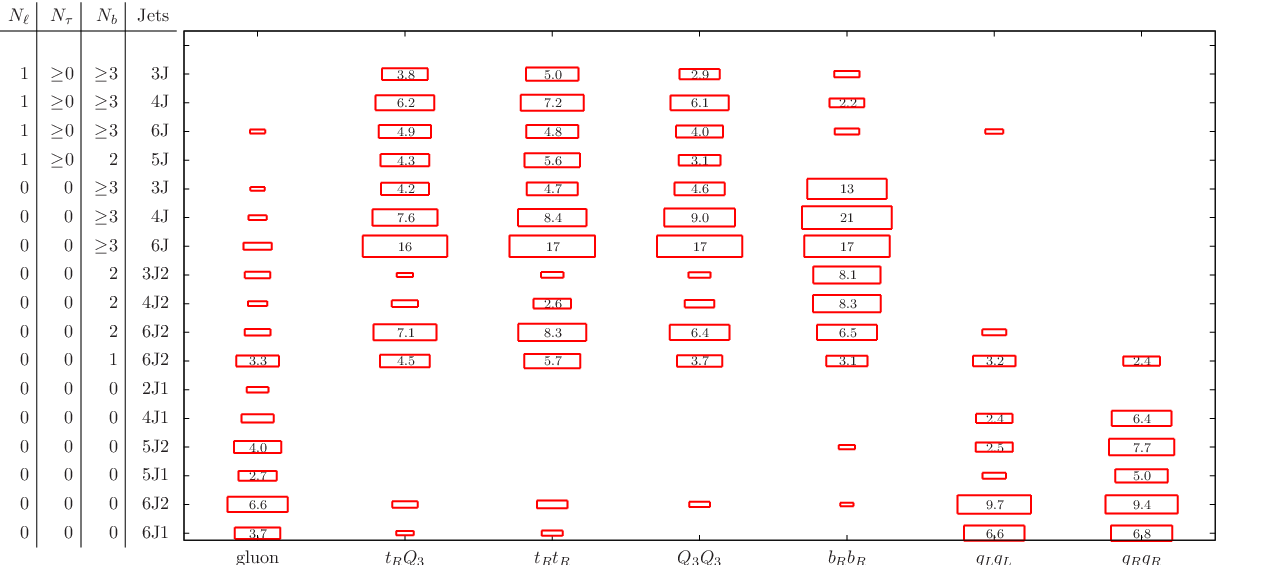
In Fig. 8, we show 1 and 2-$\sigma$ contour lines of expected parameter estimation for $B^{2}_{g}$ and $B^{3}_{q_{R}q_{R}}+B^{3}_{q_{L}q_{L}}$. Here we assume that $B(\tilde{g}\ \to g\tilde{\chi})=0.3$, $B(\tilde{g}\ \to t\bar{t}\tilde{\chi})=0.7$ and others 0 and that an integrated luminosity 25 fb^-1 at $\sqrt{s}=14$ TeV. As in the case of the simplified model, we can see there is a direction, $B^{2}_{g}+B^{3}_{q_{R}q_{R}}+B^{3}_{q_{L}q_{L}}\simeq 0.3$, in which it is slightly difficult to determine each branching fraction.

In Tab. 3, we show the expected accuracy of determination of the branching fraction of two body decay. We also show the case that some of the explanatory variables are constrained. As expected, the gluino three body decay into the first and second-family quarks mimics the signals of the gluino two body decay. With ad hoc assumption of the absence of such three body decay, a large improvement of the parameter estimation is possible. Once we get the information about the gluino decay branching fraction, we can get the stop mass from ${\cal R}_{g/t,b}$ defined in the previous section. For example, if we take $M_{1}=150~{\rm GeV}$, $M_{2}=300~{\rm GeV}$, $\mu=230~{\rm GeV}$ and $\tan\beta=2$, we can get the stop mass from the black line in Fig. 3. From Tab. 3, we can get an uncertainty $\delta{\cal R}_{g/t,b}$ is roughly given by 0.05 at $50~{\rm fb}^{-1}$. This uncertainty corresponds to the stop mass uncertainty $\delta\log m_{\rm stop}\simeq 0.7$, then, roughly, we can get the stop mass with the uncertainty of the factor 2.

Let us comment on the uncertainties from the EW-ino sector. In this study, we assume that the parameters of this sector are precisely determined. However, this is not a crucial assumption at the determination of the branching fractions. The present method mainly relies on the the third family quarks and high $P_{\rm T}$ jets from the gluino decay and not on the detail of the neutralino and chargino sector so much. Actually, we have checked that ${\cal O}(10)$% uncertainties of the parameter of the EW-ino sectors do not change the result significantly. On the other hand, at the determination of the stop mass from ${\cal R}_{g/t,b}$, Fig. 3 shows us that ${\cal O}(10)$% uncertainty about the parameters in the EW-ino sector introduces the factor 2-3 uncertainty about the stop mass. Then, we do not need the detail of the EW-ino parameters to get the order of the stop mass, however, the precise determination of the stop mass requires both the EW-ino sector information and more large luminosity. The present method is robust but crude, and there can be room for improvement. When addressing this improvement, we must deal with uncertainties from EW-ino sectors, which is out of the scope of this paper.

Another important scenario of the heavy scalar scenario is anomaly mediation models. In this model, the gaugino masses are generated from heavy gravitino mass thorough a conformal anomaly. The gaugino mass from the gravity mediation can be suppressed, if appropriate symmetry assumed. In this case, the Wino is the lightest supersymmetric particle (LSP). On the other hand, it is difficult to forbid the scalar mass generation from the gravity mediation effects by using some symmetry. Therefore a natural prediction of the AMSB model is heavier scalar mass around the gravitino mass (${\cal O}(100)\times m_{\rm gaugino}$) or more. Unlike the split SUSY case, we assume that the Higgsino mass is as heavy as the scalar particles.

In the case of the AMSB model, the charged Wino can be long-lived because of small mass difference between charged and neutralino Winos. This charged track can be detected at the LHC if a large number of SUSY particles have adequately large cross section, which is provides an important test of the AMSB model [42, 43, 44]. However, the decay length of the charged Wino is typically small ${\cal O}(1-10)$ cm and dominant signals of the AMSB models are just typical SUSY signals, i.e, large $P_{\rm T}$ jets and large missing energy. Here we focus on this dominant AMSB signals.

Let us consider the gluino decay in the AMSB model. The gluino two body decay into a neutralino and a gluon mainly comes from the Higgsino component. Thus in this AMSB case, decay $\tilde{g}\to g\tilde{\chi}_{0}$ is significantly suppressed. Therefore the AMSB predicts absence of the gluino two body decay and its confirmation provides an important test for the AMSB model. Here we discuss how well the gluino two body decay can be constrained. The gluino decay can be essentially parametrised by following branching fractions: $\tilde{g}\to g\tilde{W}^{0},g\tilde{B}^{0},t\bar{t}\tilde{W}^{0},b\bar{b}\tilde{W}^{0},tb\tilde{W}^{\pm},qq\tilde{W},t\bar{t}\tilde{B}^{0},b\bar{b}\tilde{B}^{0},q\bar{q}\tilde{B}^{0}$. As a sample point, we assume $m_{\tilde{g}}=1000$ GeV, $m_{\tilde{B}}=450$ GeV and $m_{\tilde{W}}=150$ GeV.

Using the method described previously, we constrain the gluino two body branching fraction. In Fig. 9, we show significance variables $Z$’s for some cuts for ${\cal L}=5~{\rm fb}^{-1}$ at $\sqrt{s}=14$ TeV. As in the case of the simplified model, gluino two body mode have smaller $Z$ for large jets multiplicities modes. In Table 4, we show the expected upper bound on the two body branching fraction. In this case, we can see that the gluino decay width well constrained, which gives good test for the AMSB scenario.