Planets in Open Clusters Detectable by Kepler
Abstract
Keywords:
methods: n-body simulations – methods: numerical – open clusters and associations: individual (NGC 6791) – planetary systemsWhile hundreds of planets have been discovered around field stars, only a few are known in star clusters. To explain the lack of short-period giant planets in globular clusters (GC), such as 47 Tucane and Centauri, it has been suggested that their low metallicities may have prevented planet formation. Alternatively, the high rates of close stellar encounters in these clusters may have influenced the formation and subsequent evolution of planetary systems. How common are planets in clusters around normal main-sequence stars? Here we consider whether this question can be addressed using data from the Kepler mission. The Kepler field of view contains 4 low-density (relative to GCs) open clusters where the metallicities are about solar (or even higher) and stellar encounters are much less frequent than in typical GCs. We provide detailed -body models and show that most planets in Kepler-detectable orbits are not significantly perturbed by stellar encounters in these open clusters. We focus on the most massive cluster, NGC 6791, which has super-solar metallicity, and find that if planets formed in this cluster at the same frequency as observed in the field, Kepler could detect 1 – 20 transiting planets depending on the planet-size distribution and the duration of data collection. Due to the large distance to NGC 6791 Kepler will have to search relatively faint () stars for the full extended mission to achieve such a yield.
1 Introduction
Stars are thought to always form in clusters or groups (Carpenter, 2000; Lada & Lada, 2003; Porras et al., 2003, e.g., ). Most of these clusters dissolve rather quickly under Galactic tides and via encounters with giant molecular clouds, forming the apparently isolated stars in the field. Multiple independent constraints indicate that our now-isolated star, the Sun, was born in a moderately-sized star cluster with – stars (Adams, 2010). However, this understanding leads to an apparent puzzle. Planets within a few AU from the host stars are observed to be common around normal main sequence (MS) stars in the field (Butler et al., 2006; Batalha et al., 2012, e.g.,). In contrast, few planets have been discovered around MS stars in star clusters. The only planets confirmed in star clusters to date are the Jovian-mass planet in a wide circumbinary orbit around a white-dwarf and a millisecond pulsar in M4 (Sigurdsson et al., 2003; Fregeau et al., 2006, e.g., ), the giant planet of minimum mass around Tauri, a giant star in the open cluster Hyades (Sato et al., 2007), and most recently the two hot jupiter planets around F-G stars Pr0201 and Pr0211 in Praesepe (Quinn et al., 2012). Although a number of transiting planet candidates have been reported (Mochejska et al., 2006; Lovis & Mayor, 2007; Miller et al., 2008; Pepper et al., 2008; Bruntt et al., 2003, e.g.,) around clusters stars, the planets recently discovered in Praesepe are the only planets discovered around MS stars in a star cluster. Do planets not form around cluster stars as often as around field stars? If they do form, does some physical process such as stellar encounters destroy planets with detectable orbits? Or have searches simply not been sensitive enough?
Massive () and dense clusters like typical Galactic GCs have low metallicities (Harris, 1996). Radial velocity (RV) surveys of field stars show that higher metallicity stars are more likely to host short-period giant planets (Fischer & Valenti, 2005). Thus, it has been suggested that the low metallicities of Galactic GCs may inhibit planet formation around stars in these clusters. Nevertheless, recent theoretical studies suggest that planets may be able to form even at such low metallicities, especially in short-period orbits (Hara et al., 2008; Johnson & Li, 2012, ;). Alternatively, the high interaction rates in the relatively crowded regions of star clusters may have led to the destruction of detectable planetary orbits (or close encounters may have inhibited their formation via, e.g., disk truncation). In contrast to the GCs, open clusters (typically –) have much lower central stellar densities. Analytical estimates indicate that in these lower mass clusters stellar encounters should not affect planet formation and their subsequent survival, especially for planets in orbits detectable by transit searches (Kobayashi & Ida, 2001; Adams et al., 2006, e.g., ). Of course the interaction rate depends on the planet’s semimajor axis, and a true semimajor-axis-dependent encounter frequency can only be obtained via direct -body integration of a star cluster with stars hosting planets with a large range of initial semimajor axes.
Finding a planet around a star in a low-mass cluster is challenging. These clusters dissolve at a young age under the Galactic tidal forces (Baumgardt & Makino, 2003). Therefore, the observation must be made at a relatively early age before the cluster dissolves. High precision Doppler or transit observations are not easy for young stars due to high level of star spots and stellar activity. In addition, ongoing star formation, gas expulsion, and presence of high-mass () stars in young clusters make these observations hard. Hence, an ideal star cluster for a transit search for planets should have the following properties: (1) high enough metallicity for planets to form; (2) a sufficiently massive cluster so that it does not dissolve too quickly; (3) a sufficiently old cluster so that both star and planet formation have been completed.
Searching for planets in star clusters using transit surveys has been suggested to take advantage of the high surface density of target stars (Janes, 1996). Moreover, finding the frequency of planets around cluster stars provides us with useful constraints on how often planets (within a range of semimajor axes depending on the detection limit) form, migrate, and survive around a coeval aggregate of stars. Transit surveys have been used to search for hot Jupiters in 47 Tuc, yielding a significant null result (Gilliland et al., 2000; Weldrake et al., 2005). A similar null result was found for Cen (Weldrake et al., 2008). A number of transit searches in various open clusters also revealed no convincing planet candidates around normal MS stars (Burke et al., 2006; Hartman et al., 2009; Burke et al., 2006; Mochejska et al., 2005; Mochejska et al., 2006; Miller et al., 2008; Bramich et al., 2005; Bramich & Horne, 2006; Montalto et al., 2007; Montalto et al., 2009; Rosvick & Robb, 2006, e.g., ). Nevertheless, these null results from ground based surveys do not yet constrain the planet occurrence rate in open clusters to be lower than that expected from observations in the field (van Saders & Gaudi, 2011). Hence, it would be very interesting to identify a promising candidate cluster where planets are expected to be detected. The discovery of planets in such a cluster would provide us answers to the apparent puzzle created by the presumed cluster origin of all stars, high frequency of short period planets around field stars, and the apparent lack of short period planets around cluster stars. Alternatively, a null result from that cluster would potentially put stronger constraints on planet formation efficiency in clusters than are currently present. NASA’s Kepler mission provides an unprecedented opportunity to investigate this problem due to its nearly uninterrupted photometric measurements with high cadence and precision over many years.
Four open clusters lie within the Kepler field of view (FOV), namely NGC 6866, NGC 6811, NGC 6819, and NGC 6791, in increasing order of their ages (Meibom et al., 2011). All 4 clusters have solar or higher metallicities (Platais et al., 2011; Hole et al., 2009; Gunes et al., 2012; Corsaro et al., 2012, e.g.,). Among these 4 clusters, NGC 6791 is the most massive (, Platais et al. 2011) and provides the largest number of targets to search for planets transiting normal MS stars. NGC 6791 is old (; Grundahl et al. 2008; Platais et al. 2011; Meibom et al. 2011; Brogaard et al. 2012), has super-solar metallicity ([Fe/H] = ; Boesgaard et al. 2009) and its central density is relatively low (; Platais et al. 2011), much lower than in any GC. The high metallicity indicates that planet formation in NGC 6791 should not be inhibited due to lack of metals, and the low stellar density relative to typical GCs indicates that stellar encounters are not as common as in the GCs.
In this study we use detailed -body simulations with planet-harboring stars and stellar binaries incorporating stellar evolution, two-body relaxation, Galactic tidal stripping, dynamical interactions between stars, binaries, and planetary systems, and physical collisions. Our goal is to study the semimajor axis-dependent effects of stellar encounters on planetary orbits in clusters similar to NGC 6791. Moreover, using initial distributions of planet properties based on the Kepler planet candidate list we estimate the number and properties of planets that Kepler can detect in NGC 6791 if the planet occurrence rate in this cluster is the same as that in the field.
Our numerical methods are summarized in Section 2. We present our model of NGC 6791 in Section 3. We then explore various properties indicating the effects of stellar encounters on the planetary orbits in our cluster models (Section 4) with particular focus on the model that best matches the observed properties of NGC 6791. In Section 5 we investigate whether planets in NGC 6791 can be detected by Kepler and discuss the expected properties of these detectable planets. We conclude and discuss the implications of our results in Section 6.
2 Numerical Methods
In this section we describe the code we use, how we assign cluster properties (e.g., mass, concentration, stellar binary fraction, and fraction of planet-harboring stars; Section 2.1), planetary masses and their orbital properties (Section 2.2). We describe how we estimate the expected number of Kepler-detectable planets in Section 2.3.
2.1 Modeling of NGC 6791
We model star clusters with planet hosting stars using a Hénon-type Monte Carlo code CMC (for cluster Monte Carlo) developed and rigorously tested over the past decade (Joshi et al., 2000; Joshi et al., 2001; Fregeau et al., 2003; Fregeau & Rasio, 2007; Chatterjee et al., 2010; Umbreit et al., 2012). Using this code we can efficiently model realistic clusters with a large number of star-systems () and high binary fraction () including two-body relaxation, binary and single stellar evolution, strong encounters (including physical collisions and binary mediated scattering interactions), and Galactic tidal stripping at a relatively low computational cost. These models can be directly compared with observed star clusters.
The collective effect of all of the above physical processes over the age of the cluster determines the properties of an observed cluster. Although the qualitative effects of each physical process is known, the quantitative extent of these effects are hard to estimate without doing full simulations. Hence, the initial conditions necessary to create an observed cluster cannot be easily inverted. We perform simulations for initial conditions spanning a large grid of multi-dimensional parameter space. We focus on modeling NGC 6791 and summarize a collection of properties for all other models as representative of rich open clusters. We restrict the huge parameter space to make calculations tractable. For example, NGC 6791 has a Galactocentric distance between and (Platais et al., 2011, e.g., ). It is also expected that the cluster loses about – of its initial mass via Galactic tidal stripping, dynamical ejections, and stellar evolution mass loss through winds and compact object formation (Baumgardt & Makino, 2003; Chatterjee et al., 2010, e.g., ). Considering these a priori constraints we compute a large grid of simulations varying the initial parameters including the cluster mass (), King concentration parameter (), Galactocentric distance (), and virial radius (). We compare the simulated cluster properties between – with the observed properties including the surface number density profile of NGC 6791 to find acceptable matches.
All our simulated clusters have an initial between – and an initial between –. The positions and velocities are drawn according to a King model (King, 1966; Binney & Tremaine, 2008) with between – . The initial stellar binary fraction () is chosen to be between and . We draw the masses of the stars (or primary stars in binaries) from the stellar mass function (MF) presented in Kroupa (2001, Equations 1 and 2 ) in the stellar mass range . The mass of each secondary in a stellar binary is drawn from a uniform distribution of mass ratios in the range – the mass of the primary. The initial eccentricities () are chosen to be thermal (Heggie & Hut, 2003). The initial semimajor axis () distribution is flat in logarithmic intervals between times physical contact to the local hard-soft boundary of the cluster. The local hard-soft boundary is a measure to determine the widest orbit of a stellar binary that will not be disrupted via stellar encounters in its cluster environment and depends on the velocity dispersion of the stars in the region of the cluster and the binding energy of the binary. The “hard” binaries are sufficiently bound to each other and statistically becomes more bound via super-elastic stellar encounters. On the other hand “soft” binaries are those that are not sufficiently bound and becomes less bound via stellar encounters and eventually gets disrupted via one (or multiple) stellar encounters (Heggie & Hut, 2003). Although all binaries are initially hard, they may not remain so throughout the evolution of the cluster. Due to two-body relaxation the velocity dispersion near the center of the cluster increases as the core contracts. Moreover, binaries sink to the center due to mass segregation where the velocity dispersion is higher compared to that at the initial position of a binary. We include this effect in our simulations and these soft binaries are allowed in the cluster until they disrupt via binary-single or binary-binary interactions. The orbital phase angles and orientations are chosen uniformly in the full range.
2.2 Planet properties
In addition to stellar binaries we also include stars with planetary companions determined by a planet fraction defined as the ratio of the number of planet host stars () to the number of all star systems (singles or binaries; ) in the cluster. Each primary can have only one companion in our simulations, either a stellar mass companion (we call those stellar binaries) or a planetary companion (we call those planetary binaries). Strong interactions involving both stellar binaries and planetary binaries in the evolving cluster potential are followed. In any simulation the total fraction of “binaries” (stellar and planetary) is . We do not include multiple planet systems or circumbinary (i.e., orbiting a binary star) planets due to a limitation in the current version of the code that does not allow us to treat hierarchical systems above a binary.
Planet masses () are assigned according to a power-law (Howard et al., 2010) between – where, is the mass of Jupiter. The planetary radii () are assigned a mass-dependent value according to the smaller of and , where is the radius of Jupiter (Lissauer et al., 2011). Note that although planets with are observed, we employ the upper limit in to remain conservative in our estimated number of Kepler-detectable planets (described later in Section 2.3).
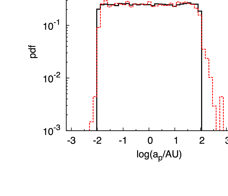
We assign the planetary orbits in two different ways, henceforth Set1 and Set2. In Set1 our focus is to find the effects of stellar encounters on planetary orbits as a function of the planetary semimajor axes () in a cluster environment. The encounter rate of a binary in a star cluster is directly dependent on its semimajor axis , and is proportional to . Hence, to estimate the -dependent effect of stellar encounters on planetary orbits we need to sample over a large range. For Set1 the initial -distribution is flat in logarithmic intervals between and . For Set1 we use a fixed value of , a somewhat arbitrary choice, but not too far from the overall fraction of Kepler planet candidates observed in the field.
Set2 consists of models with initial conditions resulting in a close match with NGC 6791 from the large grid of simulations in Set1. Here we focus on estimating the expected number of planets detectable by Kepler in NGC 6791 assuming that the initial planet frequency in the cluster is the same as observed in the field. In Set2 the orbital period distribution for planets is guided by the observed period distribution of the Kepler planet candidates (Batalha et al., 2012). Each Kepler planet candidate is weighted by , where is the radius of the host star, to account for the geometric transit probability. A lognormal distribution for orbital period is obtained by fitting the weighted Kepler planet candidate period distribution. We draw initial planet orbital periods from this lognormal distribution between and days for Set2. We use for Set2. This value of is obtained requiring that the rate of transiting planets with and period between and days is equal to the rate of Kepler planet candidates observed in the field. The Kepler planet candidate list should suffer from only minor incompleteness for planets in this range around dwarf host stars with (Batalha et al., 2012).
In all cases the initial planetary orbits are circular. Since we do not include multiple planets, there is no excitation of orbits via planet-planet scattering (Chatterjee et al., 2008, e.g., ) in our simulations. Thus, any final non-zero is a result of stellar encounters in the cluster. In (Section 4.1) we argue that indirect planet-planet instabilities, i.e., planet-planet scattering triggered by stellar fly-bys, should be a small percentage effect in clusters like NGC 6791. The orbital phase and orientation angles are drawn uniformly in the full range in both sets. Planetary companions are assigned only around host stars with in both sets since transiting planet searches focus on these systems.
2.3 Detectability of Planet Transits by Kepler
In our simulations we track single and binary stellar evolution in tandem with the dynamics (Chatterjee et al., 2010, e.g.,). Thus, at any given time in the evolution, we can extract the stellar radii () and bolometric luminosities () of planet host stars and the orbital properties of the planets. The bolometric luminosities are converted to standard colors using the standard filter band passes (Johnson , ) and synthetic stellar spectra obtained from stellar atmospheric models dependent on the stellar metallicities, and surface gravity (Lejeune et al., 1997a; Lejeune et al., 1997b). The , band magnitudes are then converted to SDSS , and magnitudes using the transformation equations from Smith et al. (2002). The Kepler magnitude is then calculated using the standard Kepler conversions obtained from the Guest Observer (GO) website of Kepler (http://keplergo.arc.nasa.gov/CalibrationZeropoint.shtml). Note that the conversion equations in the Kepler GO website is slightly different from those given in Brown et al. (2011). We find that the values calculated using the conversion equations in the Kepler GO website match better with the actual values in the Kepler target list (lower rms difference) compared to the values calculated using the equations given in Brown et al. (2011).
Whether or not a planet would be detected by Kepler depends on the ratio of the transit signal strength and the noise metric from all contributing factors (including photon noise and intrinsic stellar variability) for Kepler in a specified temporal length for the host. For a noise metric we use the combined differential photometric precision (CDPP) measured over 6.5 hours. We assign the CDPP values in ppm for the planet host stars in our simulations using a polynomial fit:
| (1) |
to the CDPP values measured by Kepler and given in Gilliland et al. (2011, their Figure 4). Note that in general extrapolating the CDPP values to large values ( needed in our study) using CDPP data in the range (Gilliland et al., 2011, given in ) can be dangerous. However, an investigation by Gilliland (private communication with the referee Gilliland) unveils that the CDPP values predicted using this extrapolation equation indeed provides CDPP values in acceptable agreement with real data even for . The values predicted by the extrapolation equation provides a more conservative estimate compared to the real data (private communication with the referee, Gilliland). The signal to noise ratio (SNR) of a transiting planet is calculated for each planet using
| (2) |
(Howard et al., 2012), where is the number of transit events within a given length of data collection by Kepler (e.g., , , and are considered), and is the duration of transit, given by
| (3) |
assuming a circular orbit and central transit. If the , we consider the planetary orbit to be “detectable” by Kepler. Each detectable planet is then weighted by the geometrical transit probability to estimate the actual number of transiting planets detected by a single observer.
The predicted number of detectable transiting planets can vary due to statistical fluctuations in their periods, sizes, and which planets were assigned to which stars in our simulations. Therefore, we vary the seed of the random number generator and generate realizations of the initial conditions for each set of cluster input parameters that gives us a good match for NGC 6791 to estimate the size of the statistical fluctuations. Note that the estimated CDPP values for a given is obtained for stars on the MS (Gilliland et al., 2011). If the CDPP values are significantly different around giant stars, then the noise metric estimated using Equation 1 may be inadequate. Nevertheless, we will show that the majority of Kepler detectable transiting planets are around bright MS stars (and some subgiant stars), hence, this caveat is not expected to be serious for the purpose of this study.
3 Simulated model of NGC 6791
| Cluster Property | Initial Value | Final Value | Observed Value | |
|---|---|---|---|---|
| All Star | ||||
| - | ||||
| Total Cluster Mass () | ||||
| Concentration parameter () | - | |||
| Virial Radius | - | - | - | |
| Galactocentric Distance () | – | |||
| Stellar binary fraction () | - | |||
| Fraction of planet-harboring stars () | - | |||
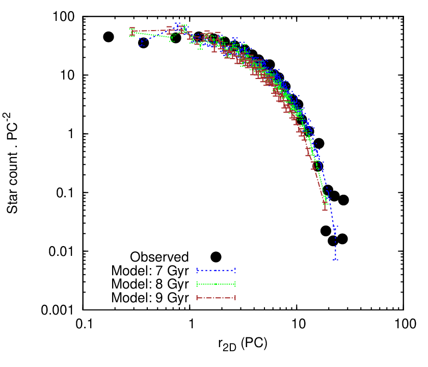
To compare our models from Set1 with the observed NGC 6791 we need to “observe” our cluster model. We compare the surface number density profiles from our models, a basic observable for clusters, with that of NGC 6791 at (Platais et al., 2011). In order to compare with the observed cluster we convert the bolometric luminosities obtained directly from CMC to standard colors using the standard filter band passes and synthetic stellar spectra obtained from stellar atmospheric models dependent on the stellar metallicities, and surface gravity (Lejeune et al., 1997a; Lejeune et al., 1997b). We only include objects brighter than to create the surface density profiles. A good match in the surface brightness profile indicates that the total luminosity (a proxy for mass) of the cluster as well as its radial distribution is well modeled. Indeed, in observed clusters the surface density profile is often used to estimate many global structural properties including central density (), core radius (), and half-light radius ().
Note that for this study we do not compare various stellar populations. Clusters are birth places for a number of exotic stellar populations including blue straggler stars (which should be created mostly via mass-transfer in a stellar binary given the low central density of NGC 6791), and low-mass X-ray binaries (Pooley & Hut, 2006). These populations depend closely on the details of the initial stellar MF, stellar binary properties, the stellar density profile, and the dynamical evolution of the cluster. While numerical modeling of star clusters focusing on reproduction of these individual exotic stellar populations is a very interesting and active area of research, it is beyond the scope of this study. For our purposes, the most important aspect in a cluster environment is its density distribution since the stellar density distribution directly affects the interaction rates and in turn affects how the properties of planetary orbits are expected to change in the cluster.

The initial conditions that produce a good match with NGC 6791 are presented in Table 1. Table 1 also lists the final properties of the model cluster at age and some observed properties of NGC 6791. Figure 1 shows the comparison between the observed surface density profile of NGC 6791 and that for our simulated best-match model at three different snapshots between .
By tracking both the dynamical evolution of the cluster objects in the overall cluster potential and the stellar and binary properties as they evolve we can create realistic synthetic color-magnitude diagrams (CMD) for our simulated models. Figure 2 shows an example of synthetic CMD created for the cluster model showing best match for the observed NGC 6791 at . The single and binary MSs, the MS turn-off, and the Giant branch are clearly visible. NGC 6791 is old (Grundahl et al., 2008, about ;) and it is relatively far from us (Platais et al., 2011, ;). Hence, the MS stars in this cluster are not very bright. Note that the single MS turn-off is at and the binary MS turn-off is near .
We summarize some key properties of all our simulated clusters in the wide multidimensional grid from our search in Table 2 available in its entirety in the electronic version. The best-match model for NGC 6791 is listed as run167 in the Table 2. In the rest of this study we will focus on the results using these cluster parameters.
| Name | () | () | |||||||
|---|---|---|---|---|---|---|---|---|---|
| run1 | 0.00 | 13.4 | 20.0 | 392.7 | 0.10 | 0.33 | 0.0006 | 0 | - |
| 0.27 | 9.1 | 19.2 | 13.7 | 0.10 | 0.33 | 0.001 | 0.03 | 0 | |
| 0.55 | 8.3 | 18.0 | 11.4 | 0.10 | 0.33 | 0.002 | 0.1 | 0.002 | |
| 0.82 | 7.6 | 16.8 | 10.7 | 0.10 | 0.33 | 0.002 | 0.2 | 0.006 | |
| 1.09 | 6.9 | 15.2 | 10.1 | 0.10 | 0.33 | 0.004 | 0.3 | 0.005 | |
| 1.36 | 6.3 | 13.6 | 9.8 | 0.10 | 0.33 | 0.004 | 0.5 | 0.005 | |
| 1.64 | 5.5 | 11.6 | 7.4 | 0.11 | 0.32 | 0.002 | 0.7 | 0.005 | |
| 1.90 | 4.7 | 9.6 | 8.0 | 0.11 | 0.32 | 0.005 | 1 | 0.005 | |
| 2.17 | 3.8 | 7.3 | 9.0 | 0.12 | 0.32 | 0.005 | 2 | 0.004 | |
| 2.45 | 2.9 | 5.3 | 9.0 | 0.12 | 0.31 | 0.009 | 3 | 0.004 | |
| 2.72 | 2.2 | 3.6 | 9.5 | 0.13 | 0.31 | 0.01 | 5 | 0.004 | |
| run2 | 0.00 | 27.1 | 40.0 | 657.9 | 0.10 | 0.33 | 0 | 0 | - |
| 0.34 | 18.4 | 39.3 | 27.4 | 0.10 | 0.33 | 0.005 | 0.01 | 0.07 | |
| pc | 0.68 | 17.4 | 38.6 | 21.0 | 0.10 | 0.33 | 0.009 | 0.03 | 0.05 |
| kpc | 1.03 | 16.6 | 37.6 | 18.7 | 0.10 | 0.33 | 0.01 | 0.06 | 0.03 |
| … | … | … | … | … | … | … | … | … | … |
4 Cluster Effects on Planets
Here we investigate the effects of stellar encounters on planetary orbits as a function of the planetary semimajor axis in open clusters similar to NGC 6791.
4.1 Stellar encounter and planetary orbits
Figure 3 shows the -distributions of the planetary objects in our numerical model of NGC 6791 (Table 1) at and . The -distribution at remains very similar to the initial distribution apart from a moderate spreading of the ranges. For the planetary orbits can shrink due to tidal damping. Moreover, stellar encounters make hard planetary orbits harder. Similarly, soft orbits expand via stellar encounters. In addition, stellar-evolution driven mass loss from the host star also expands planetary orbits. However, the overall shape of the -distribution remains more or less unchanged indicating that stellar encounters in this cluster do not significantly change most of the planetary semimajor axes with .

A more direct way to probe the importance or the lack thereof of stellar encounters in changing the planetary orbits in clusters similar to NGC 6791 is investigating the number of planets with non-zero eccentricities as a function of . We initialize all planets on circular orbits and all non-zero eccentricities are results of stellar encounters. Figure 4 shows the -distribution of planet orbits with some given value. Overall, only about of all planetary orbits acquire via interactions. Furthermore, the close-in orbits () are mostly unperturbed. Since transit surveys preferentially find planets with small semimajor axes, transit-detectable orbits are expected to remain unchanged against possible stellar encounters in clusters like NGC 6791. Thus, these orbits are not expected to be different from those in the field. We find the same general result for all our simulated models in Set1 although the exact fraction of significantly perturbed planets depends on the stellar density of the clusters (see Table 2).
Our simulations include only single planet systems. In multi-planet systems indirect instabilities may occur when a stellar encounter changes the outer planet’s orbit and this excitation in turn excites the orbits of the inner planetary system (Zakamska & Tremaine, 2004; Boley et al., 2012, e.g.,). Nevertheless, the low encounter rates even for large- orbits () indicate that such indirect instabilities should be rare and limited to a few percent effect in clusters similar to NGC 6791 (Figure 4). Of course, independent of stellar encounters, planet-planet interactions in multi-planet systems can perturb planetary orbits (Chatterjee et al., 2008; Naoz et al., 2011, e.g.,). Indeed, planet-planet interactions is a common source of perturbations for planetary systems orbiting field stars and cluster stars and the excitations due to stellar encounters serve as an additional source of perturbation in star clusters. Our simulations suggest that for clusters similar to NGC 6791, perturbations from stellar encounters should be a sufficiently small effect so that planets detectable via the transit method should not be much different from those in the field.
Even the very long-period planets ( – ) mostly remain bound to the host stars for the whole lifetime of clusters similar to NGC 6791 (Figure 3). The largest orbits have the highest interaction cross-section. These orbits are dynamically soft, resulting in further expansion of these orbits via typical stellar encounters in these clusters. In addition, stellar evolution driven mass loss further expands some of these orbits. Our simulations suggest that a small fraction of planetary orbits can expand to and still remain bound to their hosts. When such clusters dissolve near the Sun, planets with these large- orbits would populate the field and provide potential targets for direct imaging planet searches while the planets are still young and luminous.

4.2 Free-floating planets

Only a small fraction of planetary orbits are significantly perturbed (Figure 3). Most of these planets initially have large- () orbits (Figure 4). A fraction of these large- orbits can be disrupted via stellar encounters creating free-floating planets. Mass segregation drives the free-floating planets away from the cluster center, but the free-floating planets can remain bound to the cluster potential for many relaxation times near the outskirts of the cluster (Hurley & Shara, 2002). In our simulations we find that these free-floating planets reside near the tidal boundary of the cluster confirming previous results. Some free-floating planets can remain bound to the cluster for a few billion years after formation. Since the free-floating planets leave the core of the cluster due to mass segregation quickly, further interaction of free-floating planets with other planetary orbits is unlikely.
The number of free-floating planets generated by stellar encounters remains low (), a direct effect of low encounter rates in these clusters. This number depends on the actual number of planets with sufficiently wide orbits for interaction with other stars or binaries in the cluster. Hence we define a quantity , where is the number of planets bound to hosts in the cluster, the same but with orbits wider than , and is the number of free-floating planets bound to the cluster potential. For clusters similar to NGC 6791 remains a few percent for all times. In denser clusters in our simulations can be as high as . At by construction. In general, grows until an age followed by a steady decrease as the cluster grows older due to preferential stripping of free-floating planets via Galactic tides (Table 2).
Microlensing surveys indicate that there is a large number of free-floating (or wide orbit) planets in the Galaxy (Sumi et al., 2011). Microlensing surveys have also detected planetary mass candidates in the young open clusters Orionis and Orion (Zapatero Osorio et al., 2000; Zapatero Osorio et al., 2002; Bihain et al., 2009). Hence, it is interesting to investigate what fraction of wide planetary orbits are disrupted to create free-floating planets that may or may not remain bound to the cluster. For this purpose we define a quantity , where is the total number of free-floating planets (bound to and escaped from the cluster), and is the initial number of wide planetary orbits. Figure 5 shows the distribution for for all our simulated cluster models and for all cluster ages. The values of are typically about a few percent for our simulated models. Thus, if stellar encounters dominate production of free-floating planets then most microlensing planets are likely wide orbit planets, rather than free-floating planets. However, note that this is a lower limit for for clusters similar to our simulated models. The actual number of free-floating planets could be significantly higher due to the contribution from planet-planet scattering in multi-planet systems (Chatterjee et al., 2008, e.g.,).
4.3 Number of planets and cluster age
The total number of star systems (single and stellar or planetary binaries) bound to the cluster steadily decreases over time due to Galactic tidal stripping. As a result the total number of planets in the cluster also steadily decreases over time. However, the ratio of planet host stars in the cluster to all star systems in the cluster () remains roughly constant (Table 2). For dissolving clusters the ratio grows with time, where, is the number of planets escaped from the cluster potential. In our simulations, can become very large depending on the cluster age and properties ( e.g., run145). For a completely dissolved cluster the limiting value is . For our best-match model of NGC 6791 at a cluster age (run167, Table 2). Thus, for every planet in this cluster there are planets that are now in the field due to the slow dissolution of the cluster.
This decrease in is dominated by the host being lost from the cluster. The number of planets lost from the cluster still bound to their host stars is typically times the number of free-floating planets lost from the cluster at all cluster ages (Figure 6). This is simply because complete ionization of planetary orbits is not common in clusters such as NGC 6791 even for the broad range in considered in our simulations in Set1. The fraction of free-floating escaped planets with respect to escaped planets still bound to their hosts () are given in Table 2 for all our simulated clusters at various ages. Note again that the fraction of free-floating planets in the field presented here is a lower limit based solely on the stellar interactions in the cluster of origin for the planet-host stars and does not account for possible contribution from planet-planet scattering.
5 Detectability of planets in NGC 6791 using Kepler
We have established that stellar dynamics in clusters similar to NGC 6791 alone cannot significantly alter small- planetary orbits that are detectable via transit surveys like Kepler. In addition, we know that NGC 6791, already in the Kepler FOV, has super-solar metallicity (Platais et al., 2011). Hence, formation of planets should not be reduced due to lack of solids in protoplanetary disks in this cluster. Now we use the simulations from Set2 (Section 2) to estimate how many planets Kepler could discover in NGC 6791 assuming that planets form around cluster stars at the same frequency as observed in the field by Kepler and that their initial planetary orbits have similar properties to those orbiting around field stars. Note that initially we do not include any boost in planet occurrence rate due to the super-solar metallicity of NGC 6791 (Fischer & Valenti, 2005). We discuss briefly the estimated effects of the high metallicity of NGC 6791 on the predicted number of planet detections later in Section 5.2. The initial conditions for our models in Set2 are taken from the best-match model in Set1 (Table 1). Set2 consists of different realizations of the same initial cluster. The period distribution of the planets follow the distribution seen in the Kepler planet candidate list after de-biasing for transit probability (Batalha et al., 2012). Initially we consider a planet mass distribution estimated from the RV surveys. However, later in this section (Section 5.2) we explore how the results would change if we adopt other planet size distributions including ones based on Kepler observations. The is chosen based on the observed field planet occurrence rate (Section 2.2).

Figure 7 shows a cumulative histogram of the number of transiting planets () detectable by Kepler as a function of the Kepler magnitude. is near the MS turn-off of NGC 6791 (Figure 2) and the steep rise in near is reflective of the stellar properties in the cluster. Although the giants () are much brighter than the MS stars, they are less numerous. In addition, the giants also have a much larger . Hence the transit is not sufficient for most planets to be detected around these giant stars. However, there is a chance that Kepler may detect a few giant planets around low-luminosity giant stars. Most planet detections in NGC 6791 with Kepler will be around high-luminosity MS star hosts (). Our results suggest that if planet occurrence rate in NGC 6791 is similar to that observed in the field, Kepler could detect a few to planets depending on the adopted planet-size distribution even with a single year of data collection. A total of about – and – planets are expected to be detected from and of data collection by Kepler. These ranges reflect uncertainties from the planet-size distribution (Table 3). Relatively faint stars () must also be analyzed to achieve this yield. The lack of detections of Kepler candidates in this cluster to date may be due to inadequate analysis of these faint target stars.

Figure 8 shows the cumulative number of transiting planets detectable by Kepler in NGC 6791 as a function of the planetary radius (). About and of all Kepler-detectable planets are expected to be larger than Saturn and Neptune, respectively, if 1 year of data is analyzed. Increasing the duration of analyzed Kepler data increases the number of detections for smaller planets. For example, the median for the predicted number of Kepler-detectable planets is about , , and when analyzing , , and of Kepler data, respectively. The expected numbers of detectable planets with are about , , and when analyzing , , and of Kepler data, respectively. Note that the actual numbers of detections may be higher or lower by a few planets due to statistical fluctuations as shown by the shaded regions in Figures 7 and 8. The sharp increase in the detectable planet numbers in the bin is reflective of our assumed mass-to-radius relation which does not allow our planets to have (Section 2). Without this assumption some of the planets in this bin would spread into bins with larger radii. Almost all detectable planets for , , and observations are expected to be in orbits with periods below about , , and days, respectively.

Figure 9 shows the cumulative number of Kepler-detectable planets as a function of the sky-projected distance from the center of the cluster. Most Kepler-detectable planets are not in the most concentrated part of the cluster near the center. In fact, only about of detectable planets are expected to reside inside the projected of the cluster. A little over of the detectable planets are expected to reside outside the projected half-light radius of the cluster. This is due to mass segregation in the cluster and does not include observational selection effects due to crowding.
In general, crowding of stars can become a potential problem for transit searches in a star cluster. The extent of crowding for each star in the Kepler FOV depends on the number of pixels enclosing of the star’s flux (EE95). The EE95 values for the module containing NGC 6791 in the Kepler FOV varies between – pixels (obtained from the Kepler Instrument Handbook; http://keplergo.arc.nasa.gov/calibration/KSCI-19033-001.pdf) depending on the quarter of observation. Adopting EE95 of pixels and an angular scale per pixel of arcseconds (Bryson et al., 2010, equivalent to an area of about at the distance of NGC 6791;), the number density of stars with in NGC 6791 is at a cluster-centric two dimensional () projected distance () of about ( if EE95 is pixels; Figure 9). Between – of all otherwise detectable planets in our simulations reside outside – – . Even at the center of NGC 6791 the number of stars per pixel is . Hence, crowding should not be a fundamental limit for planet search in NGC 6791 using Kepler. However, the current pipeline may not be sufficient due to technical issues associated with targeting and analysis of stars in a dense field.
The above estimated numbers of Kepler-detectable planets in NGC 6791 can change based on various parameters including the intrinsic planet frequency, the planet-size distribution, metallicity of NGC 6791, limited data availability and crowding. The effect of the assumed intrinsic planet-occurrence frequency, denoted by in this study, on the number of detectable transits is straightforward. If all other parameters such as the period distribution and the planet-size distribution are kept fixed, the number of transit detections by Kepler simply scales linearly with . In the following sections we discuss the effects of the other parameters on the number of detectable transits by Kepler in NGC 6791.
5.1 Effects of planet-size distribution
For a fixed , estimating the change in the number of Kepler detectable planets depending on the distribution of planet sizes is relatively more complicated. Assuming that the planet size distribution is described by a simple power-law of the form , we estimate the dependence of the number of expected transit detections by Kepler in NGC 6791 as a function of the power-law exponent in the following way. We extract the planet-harboring stars in our simulations at but now change the planetary sizes based on several different power-law distributions. For each value of , realizations are generated to estimate the statistical fluctuations. Each of these planetary systems are then analyzed using the same method described in Section 2.3. We use a range of values spanning those reported in literature. We report the expected number of transit detections in NGC 6791 by Kepler as a function of in Table 3. Depending on the value of , the expected number of detections can have values over an order of magnitude.
| Number of Detected Transits | Comments | |||
|---|---|---|---|---|
| 1 year | 3.5 year | 8 year | ||
| - | ||||
| these simulations; Howard et al. (2010) | ||||
| Youdin (2011) | ||||
| Howard et al. (2012) | ||||
| - | ||||
5.2 Effects of metallicity
The planet occurrence rate varies with the metallicity of the target stars (Fischer & Valenti, 2005). NGC 6791 has a super-solar metallicity ([Fe/H] = +0.30; Boesgaard et al. 2009). Analysis up to this point did not account for the fact that the high metallicity of NGC 6791 is likely to boost planet occurrence in this cluster relative to the Kepler target list. The correlation between planet occurrence and metallicity is well established for giant planets (Fischer & Valenti, 2005; Valenti & Fischer, 2008; Santos et al., 2011, e.g.,) but is not as strong for planets smaller than (Sousa et al., 2011; Buchhave et al., 2012, e.g.,). Here we explore how much the super-solar metallicity of NGC 6791 could change the estimated number of detectable transiting planets by Kepler in this cluster. To remain conservative we assume that the planet frequency is increased due to metallicity only for planets larger than Saturn. We further assume that the distributions of orbital properties (e.g., period distribution) of hot jupiters are independent of the metallicity.
Based on the RV observations Fischer & Valenti (2005) fit for the planet occurrence rate and the metallicity of the host stars and find
| (4) |
where, denotes the number of atom x per unit volume, is the planet occurrence rate at Solar metallicity, and is the planet occurrence rate as a function of the metallicity of the host star. We call this Function1. To estimate the planet occurrence rate in NGC 6791 we also consider
| (5) | |||||
which we call Function2. Here we assume that the planet occurrence rate with respect to the metallicity increase as a power-law as found by Fischer & Valenti (2005) only for Solar or higher metallicities and is flat below Solar metallicities. For both cases the average planet occurrence rate is calculated considering all Kepler targets using . The expected planet occurrence rate is also calculated for NGC 6791 using [Fe/H] = +0.30 (Boesgaard et al., 2009). The boost of planet occurrence rate for giant planets larger than Saturn is then simply . We find that this ratio is and assuming Function1 and Function 2, respectively.
If the super-solar metallicity boosts the planet occurrence rate for all planet sizes, then the total number of detectable transits will simply scale with the numbers presented in Table 3. If the planet occurrence rate is boosted by the above factors in NGC 6791 only for giant planets (i.e., larger than Saturn), the expected number of transit detections will increase by a smaller factor depending on the number of giant planets, which in turn depends on the planet-size distribution. Table 4 shows the expected numbers of transit detections by Kepler boosted due to the super-solar metallicity of NGC 6791 assuming that the planet occurrence rate is boosted only for giant planets larger than Saturn and that the planet-size distribution is described by a power-law with exponent .
| (yr) | Relation | All Cluster | Downloaded Cluster | |||||
|---|---|---|---|---|---|---|---|---|
| Unboosted | Boosted | Unboosted | Boosted | Unboosted | Boosted | |||
| Function1 | ||||||||
| (Equation 4) | ||||||||
| Function2 | ||||||||
| (Equation 5) | ||||||||
5.3 Effects for finite data download by Kepler

Our analysis in Section 5 shows that the best chance for Kepler to detect transits in NGC 6791 is around bright MS stars (; Figure 7). All predicted numbers of transit detections from our simulations in Sections 5.1 – 5.2 have been calculated assuming that data for all stars in NGC 6791 up to is available. In practice, not all needed pixels are downloaded. Kepler has been observing a few regions in the FOV through large, custom apertures where pixel level data is downloaded. These are called “superapertures” (http://keplergo.arc.nasa.gov/Blog.shtml). In particular for NGC 6791 a superaperture of pixels block centered on the cluster center is being downloaded (Stello et al., 2011, e.g.,). In addition to this superaperture data, data from about individual stars consistent to be MS stars in NGC 6791 (i.e., within the tidal radius of the center of NGC 6791, magnitude , and surface gravity ) are being downloaded by Kepler. Most of these individual stars with downloaded data are already included in the superaperture (Figure 10). The right panel of Figure 10 shows the superaperture block, and the individual stars consistent to be MS stars in NGC 6791 for which data is available (or will become available as part of a GO proposal). Important cluster structural radii (, , and ) are also shown. The left panel shows a two dimensional image of our simulated model of NGC 6791 over-plotted with the superaperture block, and the above mentioned cluster radii. Detectable transits by Kepler will be around bright main-sequence dwarf stars in NGC 6791. Thus at the given age of NGC 6791 these host stars are among the lower-mass sub-population of the cluster (). Mass-segregation distributes these relatively lower mass stars at larger cluster centric distances compared to the stellar binaries and more-massive (and evolved) single stars in NGC 6791. Thus while red giants are predominantly near the center of the cluster, a large fraction () of transit detectable planet host stars are outside . Ideally, the best place to search for these planets is between and . However, due to the limited data availability this cannot be done. We find that between – and the superaperture box ( along a side of the square and along a diagonal) transits could be detectable by Kepler with one year of data collection assuming and no metallicity boost. Table 4 lists the expected numbers (with and without metallicity boost) of transit detections for different observations lengths in different cluster regions (including the region between and the superaperture box). However, note that most of the stars in the superaperture are not analyzed as part of the regular planet search pipeline.
6 Discussion

We revisit the possibility of detecting planets around normal MS stars in clusters in the light of the highly successful Kepler mission. In particular, we focus on NGC 6791, an old, massive, and metal-rich open cluster. The fact that NGC 6791 is already being observed by Kepler makes it an ideal candidate to test hypotheses developed to explain previous planet searches that report a dearth of planets around normal MS stars in clusters.
Using detailed numerical simulations of a cluster’s evolution and planet-harboring stars we study effects of stellar encounters in rich open clusters. We choose a model that best matches the observed properties of NGC 6791 from this large set of simulations performed on a broad multidimensional grid of initial conditions (Section 3, Table 1, Figure 1). We find that planetary orbits are rarely disrupted solely via stellar encounters in open clusters for a large range in cluster mass and stellar density (Table 2). For clusters similar to NGC 6791, only about 10% of planetary orbits with relatively large semimajor axes () are likely to be excited via strong stellar encounters (Figure 4). A small fraction () of large- orbits may get ionized (Table 2). However, the bulk of the planetary orbits, especially the small- orbits (), detectable via transit searches, remain undisturbed (Figures 3 and 4).
We find that the number of free-floating planets can range from a few to in a cluster like NGC 6791 depending on the age of the cluster. In our best-match model of NGC 6791 the highest fraction of free-floating planets bound to the cluster potential, , grows from an initial value of zero by construction to the maximum value of (Table 1). However, depending on the cluster properties and age can be higher (Figure 5; Table 2). The total number of planets in a cluster steadily decreases with the age of the cluster mainly due to Galactic tidal stripping of the host stars (Figure 6). These planet-host stars then leave the cluster to populate the field. Planetary orbits with (and up to in our simulations) can remain bound to the host stars in a cluster similar to NGC 6791 (Figure 3).
6.1 Prospects for cluster-planet detection from Kepler
We estimate the expected number of planets Kepler may discover in NGC 6791 using the best-match initial conditions obtained from our grid of simulations to create models of NGC 6791 with planet frequency and planetary properties (Section 2.2) guided by the current Kepler observations in the field (Batalha et al., 2012). If the planet occurrence rate in NGC 6791 is the same as observed in the field by Kepler, then the existing Kepler data could detect transits of between a few to planets (Figure 7, Table 3) depending on the intrinsic distribution for planet sizes analyzing 1 year of data. An extended Kepler mission over (or more) is projected to increase this yield by a factor of 2. However, due to the old age () and large distance () of NGC 6791, most of these detectable-planet-host stars are relatively faint (, the MS turn-off for NGC 6791; Figure 2). Hence, to attain such an yield, Kepler data for relatively faint stars () must be analyzed properly. These numbers are expected to increase due to the high metallicity of NGC 6791 (Fischer & Valenti, 2005, given the positive correlation between the intrinsic planet occurrence rate and the metallicity of the host stars, e.g.,) (Table 4). On the other hand, since data is not available for all stars in NGC 6791 the actual number of transit detection will be reduced (Table 4).
Although a few giant planets may be detectable around low-luminosity giant stars, most planets should be detected around MS stars close to the MS turn-off (Figure 7). When using only observation by Kepler a large fraction () of the detected planets will likely be gas giants. With longer observation times the expected number of detections for smaller planets grows and the median of detected planets decreases from after to about after (for a planet-size distribution with ; Table 3). With an extended mission of a few transits of planets as small as could be detected in NGC 6791 (Figure 8).
About of the detectable planets are expected to reside outside the core () of NGC 6791, and a little above of the detectable planets are expected to reside outside the half-light radius () of NGC 6791 (Figure 9). Between – of all otherwise detectable planets reside outside the projected distance – from the cluster center beyond which the number of stars per EE95 is less than 1. Hence, crowding should not be a limiting factor in the detection of planets in NGC 6791 using Kepler, once the data between and the superaperture boundaries ( along a side and along a diagonal) is fully analyzed.
Note that the MS planet hosts, are among the lower mass ()
subpopulation in the cluster given the old age of NGC 6791.
Hence mass segregation distributes them at relatively larger separations
from the cluster center compared to the stellar binaries and more massive evolved stars
(Section 5). Ideally, the best place to search for transits in this cluster would be between
(to avoid crowding) and (since there are simply not many stars
beyond this radius). Hence, based on our results we suggest the following.
1. Relatively fainter stars () should also be properly analyzed.
2. Ongoing observations of the clusters in the Kepler FOV, especially the relatively massive clusters
NGC 6791 and NGC 6819 are maintained not only for astrophysics, but also to search for exoplanets.
3. The pixel-level data obtained from the superapertures are analyzed for existence of transiting planets.
Especially, data for regions outside where there is reduced crowding.
4. For detection of exoplanets it is more important to get data from the outer (e.g., outside the ) regions of
a cluster. Considering the limitation of the number of pixels that can be downloaded,
we suggest that some pixels
from the center of the superapertures be reassigned to search for planets around individual MS stars
likely to be cluster members and located outside the superaperture block.
Kepler results can determine whether planets in short period orbits are as common around cluster stars as they are around field stars. Even a null result from Kepler would be interesting since that would potentially provide stronger constraints than the existing results on the frequency of planet occurrence around MS stars in star clusters.
6.2 How likely is a planet discovered near a cluster an actual cluster member?
In Figure 11 we show a preliminary analysis of the Kepler planet candidates near star clusters as a function of their sky positions relative to a cluster. Planet candidates are from (Batalha et al., 2012) and are based on searching Kepler data from Q1–Q6. The top panels show the region around NGC 6791 only, and the bottom panels combine the regions around four open clusters (NGC 6866, NGC 6811, NGC 6819, and NGC 6791) in the Kepler FOV. We plot the number of observed Kepler candidates () as a function of the projected distance from the cluster center(s). The cluster-centric distances are given in units of the cluster’s tidal radius(ii) (). Cluster parameters, including positions, tidal radii, distances, ages, and redennings are taken from the literature (Kalirai et al., 2001; Kharchenko et al., 2005; Hole et al., 2009; Piskunov et al., 2008; Platais et al., 2011, WEBDA) The observed points are drawn for three sets of target stars defined in the following way. In the left panels we include all stars with that were observed by Kepler. In the middle panels we limit the sample to include only stars with contamination to reduce the effect that stray light from nearby stars may have on the frequency of Kepler candidates, which may be significant in clusters like NGC 6791. This value of is chosen fairly arbitrarily, and a more thorough analysis is needed to determine the proper cutoff in to draw robust conclusions. Finally, in the right panels, we limit the Kepler sample to only include stars that would lie between the single-star and equal-mass binary sequences of the respective clusters. We use Marigo et al. (2008) isochrones in log() vs. space to perform this selection.
Although the vast majority of the Kepler observed stars (and especially those targeted for the “EX” program) have , we include all stars with observed by Kepler to remain consistent with our theoretical expectation that planets have the highest detection probability between in NGC 6791. Given the old age and distance of NGC 6791, the cluster MS begins at (Figure 2). Consequently, the majority of the observed Kepler candidates in Figure 11 for NGC 6791 must be giants, or possibly subgiants, if they are really around cluster members. Our numerical models suggest that it is unlikely for Kepler to detect more than about planets around giant host stars in NGC 6791 (Figure 7). Kepler has not yet reported strong planet candidates transiting stars that are within from the center of NGC 6791 and have magnitudes and temperatures consistent with a MS cluster member (top-right panel of Figure 11). Given that our models predict significantly more planet detections possible by Kepler for the MS stars in NGC 6791, we suggest that a detailed analysis of these fainter stars for planet transits would be highly valuable.
If a transit is detected in the direction of a cluster, it is not a priori clear whether the planet is indeed around a cluster star or around a foreground/background star. We find that if a transiting planet is detected within from the center of NGC 6791 and the host star has properties such that it will lie within the single and equal-mass binary MSs in the CMD of NGC 6791, then the planet is very likely to be around a true cluster member. About of all transiting planet detections around stars satisfying this criteria and within from the center of NGC 6791 are expected to be around true cluster members (Figure 11, top-right). Given that there are about 10 Kepler candidates within the tidal radii of the 4 open clusters in the Kepler FOV (Figure 11, bottom-right) around stars with properties satisfying the CMD based limits described above, about of these systems may be true cluster members. The relative contributions from the cluster stars and the foreground/background stars do not change significantly if the power-law exponent for the planet-size distribution is changed in the range explored in this study (Table 3). However, note that this part of the analysis has a few caveats as described below.
We compute the predicted number of Kepler detectable planets transiting foreground/background stars superimposed on our model of NGC 6791 (thin lines in the top panels of Figure 11). To produce these curves, we embed the simulated cluster within a uniform field of background/foreground stars and treat these data in the same manner as for the Kepler observations. We use the Besançon model of the Milky Way (Robin et al., 2003) to estimate the -dependent surface densities of stars in the direction of NGC 6791. Using the transformation equations from Smith et al. (2002) we convert the Johnson , magnitudes given in the Besançon model to SDSS , , and then use the standard Kepler conversions to find . We estimate the surface densities of background/foreground stars in the direction of NGC 6791 as a function of . The surface density of the expected Kepler detections for planets transiting these background/foreground stars per solid angle is then estimated using the same method described in Section 2 for values between . These estimated surface densities are then summed to obtain the integrated surface density of planet detections for non-cluster stars over the full range in . The expected cumulative number of transit detections for non cluster stars as a function of the distance () from the cluster center is then found simply by multiplying the expected number of transit detections per sky-projected area and .
We find that the total number of background/foreground stars estimated from the Besançon model can be lower by than that counted from the Kepler Input Catalog (KIC) by centering at the same Galactic latitude but away from the cluster. Even the numbers of stars estimated from the KIC catalog using a center at different nearby locations at the same Galactic latitude can vary by about . These differences in the number of stars are directly translated to differences in the estimated number of detectable transits around non cluster members. For example, using the KIC stars within an angular radius of centered around a point away from NGC 6791 but at the same Galactic latitude as NGC 6791, this model would estimate an expected number of detectable planets within , transiting non cluster stars with to be . Using the same cut-offs for and , but using the Besançon model the estimated number of detectable transiting planets is . We caution that, both of the above estimates are likely upper limits on the number of detectable planets transiting non-cluster stars, since it assumes that all non-cluster stars are dwarfs. A significant fraction of the foreground/background stars will be giant or subgiant stars for which the minimum detectable planet size is significantly larger than for a MS star of the same magnitude. Thus, the thin lines should be treated as rough estimates for an upper limit to the number of contaminating planets around foreground/background stars. Fortunately, even these results suggest that planet candidates within are likely cluster members if the selected sample has properties consistent with their being on the MS of the cluster.
A more complete and careful study of the frequency of planets in the fields near the open clusters in the Kepler survey is of great interest (but beyond the scope of this paper). We stress here that a complete study of any putative trend between planet occurrence rate and position relative to a cluster must be mindful of a number of caveats (in addition to those mentioned above) related to how the sample of target stars are chosen before drawing secure conclusions. For example, the search for planets in clusters is still incomplete (for NGC 6791 it has barely started) due to technical details related to targeting and the pipeline. A careful study must include proper cuts in the values to fairly compare cluster stars with those in the field, and take into account differences in magnitude, stellar radii, contamination, pipeline selection effects between cluster and field stars, and preferably kinematic cluster membership information.
Acknowledgmentes: We thank the referee, R. Gilliland, for a detailed review and many helpful suggestions and information. We thank S. Meibom for helpful discussion. We thank D. Stello, A. V. Tutukov, K. F. Brogaard, for helpful suggestions and comments based on the preprint. SC acknowledges support from the Theory Postdoctoral Fellowship from UF Department of Astronomy and College of Liberal Arts and Sciences. This material is based on work supported by the National Aeronautics and Space Administration under grant NNX08AR04G issued through the Kepler Participating Scientist Program. All cluster simulations using CMC were performed using the computer cluster fugu at Northwestern University. F.A.R. acknowledges support from NASA Grant NNX12AI86G.
References
- Adams (2010) Adams F. C., 2010, ARA&A, 48, 47
- Adams et al. (2006) Adams F. C., Proszkow E. M., Fatuzzo M., Myers P. C., 2006, ApJ, 641, 504
- Batalha et al. (2012) Batalha N. M., et al. 2012, arXiv: 1202.5852 astro-ph.EP
- Baumgardt & Makino (2003) Baumgardt H., Makino J., 2003, MNRAS, 340, 227
- Bihain et al. (2009) Bihain G., et al. 2009, A&A, 506, 1169
- Binney & Tremaine (2008) Binney J., Tremaine S., 2008, Galactic Dynamics: Second Edition. Princeton University Press
- Boesgaard et al. (2009) Boesgaard A. M., Jensen E. E. C., Deliyannis C. P., 2009, AJ, 137, 4949
- Boley et al. (2012) Boley A. C., Payne M. J., Ford E. B., 2012, arXiv:1204.5187v1 [astro-ph.EP]
- Bramich & Horne (2006) Bramich D. M., Horne K., 2006, MNRAS, 367, 1677
- Bramich et al. (2005) Bramich D. M., Horne K., Bond I. A., Street R. A., Collier Cameron A., Hood B., Cooke J., James D., Lister T. A., Mitchell D., Pearson K., Penny A., Quirrenbach A., Safizadeh N., Tsapras Y., 2005, MNRAS, 359, 1096
- Brogaard et al. (2012) Brogaard K., et al. 2012, A&A, 543, A106
- Brown et al. (2011) Brown T. M., Latham D. W., Everett M. E., Esquerdo G. A., 2011, AJ, 142, 112
- Bruntt et al. (2003) Bruntt H., Grundahl F., Tingley B., Frandsen S., Stetson P. B., Thomsen B., 2003, A&A, 410, 323
- Bryson et al. (2010) Bryson S. T., Tenenbaum P., Jenkins J. M., Chandrasekaran H., Klaus T., Caldwell D. A., Gilliland R. L., Haas M. R., Dotson J. L., Koch D. G., Borucki W. J., 2010, ApJ, 713, L97
- Buchhave et al. (2012) Buchhave L. A., et al. 2012, Nature, 486, 375
- Burke et al. (2006) Burke C. J., Gaudi B. S., DePoy D. L., Pogge R. W., 2006, AJ, 132, 210
- Butler et al. (2006) Butler R. P., Wright J. T., Marcy G. W., Fischer D. A., Vogt S. S., Tinney C. G., Jones H. R. A., Carter B. D., Johnson J. A., McCarthy C., Penny A. J., 2006, ApJ, 646, 505
- Carpenter (2000) Carpenter J. M., 2000, AJ, 120, 3139
- Chatterjee et al. (2008) Chatterjee S., Ford E. B., Matsumura S., Rasio F. A., 2008, ApJ, 686, 580
- Chatterjee et al. (2010) Chatterjee S., Fregeau J. M., Umbreit S., Rasio F. A., 2010, ApJ, 719, 915
- Corsaro et al. (2012) Corsaro E., et al. 2012, arXiv:1205.4023 [astro-ph.SR]
- Demleitner et al. (2001) Demleitner M., Accomazzi A., Eichhorn G., Grant C. S., Kurtz M. J., Murray S. S., 2001, in Harnden Jr. F. R., Primini F. A., Payne H. E., eds, Astronomical Data Analysis Software and Systems X Vol. 238 of Astronomical Society of the Pacific Conference Series, ADS’s Dexter Data Extraction Applet. p. 321
- Fischer & Valenti (2005) Fischer D. A., Valenti J., 2005, ApJ, 622, 1102
- Fregeau et al. (2006) Fregeau J. M., Chatterjee S., Rasio F. A., 2006, ApJ, 640, 1086
- Fregeau et al. (2003) Fregeau J. M., Gürkan M. A., Joshi K. J., Rasio F. A., 2003, ApJ, 593, 772
- Fregeau & Rasio (2007) Fregeau J. M., Rasio F. A., 2007, ApJ, 658, 1047
- Gilliland et al. (2011) Gilliland R. L., Chaplin W. J., Dunham E. W., Argabright V. S., Borucki W. J., Basri G., Bryson S. T., Buzasi D. L., Caldwell D. A., Elsworth Y. P., Jenkins J. M., Koch D. G., Kolodziejczak J., Miglio A., van Cleve J., Walkowicz L. M., Welsh W. F., 2011, ApJS, 197, 6
- Gilliland et al. (2000) Gilliland R. L., et al. 2000, ApJ, 545, L47
- Grundahl et al. (2008) Grundahl F., Clausen J. V., Hardis S., Frandsen S., 2008, A&A, 492, 171
- Gunes et al. (2012) Gunes O., Karatas Y., Bonatto C., 2012, arXiv:1205.2760 [astro-ph.GA]
- Hara et al. (2008) Hara T., Kunitomo S., Shigeyasu M., Kajiura D., 2008, in Y.-S. Sun, S. Ferraz-Mello, & J.-L. Zhou ed., IAU Symposium Vol. 249 of IAU Symposium, On the formation age of the first planetary system. pp 325–328
- Harris (1996) Harris W. E., 1996, AJ, 112, 1487
- Hartman et al. (2009) Hartman J. D., Gaudi B. S., Holman M. J., McLeod B. A., Stanek K. Z., Barranco J. A., Pinsonneault M. H., Meibom S., Kalirai J. S., 2009, ApJ, 695, 336
- Heggie & Hut (2003) Heggie D., Hut P., 2003, The Gravitational Million-Body Problem: A Multidisciplinary Approach to Star Cluster Dynamics. Cambridge University Press, 2003
- Hole et al. (2009) Hole K. T., Geller A. M., Mathieu R. D., Platais I., Meibom S., Latham D. W., 2009, AJ, 138, 159
- Howard et al. (2012) Howard A. W., et al. 2012, ApJS, 201, 15
- Howard et al. (2010) Howard A. W., Marcy G. W., Johnson J. A., Fischer D. A., Wright J. T., Isaacson H., Valenti J. A., Anderson J., Lin D. N. C., Ida S., 2010, Science, 330, 653
- Hurley & Shara (2002) Hurley J. R., Shara M. M., 2002, ApJ, 565, 1251
- Janes (1996) Janes K., 1996, J. Geophys. Res., 101, 14853
- Johnson & Li (2012) Johnson J. L., Li H., 2012, arXiv:1203.4817 [astro-ph.EP]
- Joshi et al. (2001) Joshi K. J., Nave C. P., Rasio F. A., 2001, ApJ, 550, 691
- Joshi et al. (2000) Joshi K. J., Rasio F. A., Portegies Zwart S., 2000, ApJ, 540, 969
- Kalirai et al. (2001) Kalirai J. S., Richer H. B., Fahlman G. G., Cuillandre J.-C., Ventura P., D’Antona F., Bertin E., Marconi G., Durrell P. R., 2001, AJ, 122, 266
- Kharchenko et al. (2005) Kharchenko N. V., Piskunov A. E., Röser S., Schilbach E., Scholz R.-D., 2005, A&A, 438, 1163
- King (1966) King I. R., 1966, AJ, 71, 64
- Kobayashi & Ida (2001) Kobayashi H., Ida S., 2001, Icarus, 153, 416
- Kroupa (2001) Kroupa P., 2001, MNRAS, 322, 231
- Lada & Lada (2003) Lada C. J., Lada E. A., 2003, ARA&A, 41, 57
- Lejeune et al. (1997a) Lejeune T., Cuisinier F., Buser R., 1997a, VizieR Online Data Catalog, 412, 50229
- Lejeune et al. (1997b) Lejeune T., Cuisinier F., Buser R., 1997b, A&AS, 125, 229
- Lissauer et al. (2011) Lissauer J. J., et al. 2011, arXiv:1102.0543 [astro-ph.EP]
- Lovis & Mayor (2007) Lovis C., Mayor M., 2007, A&A, 472, 657
- Marigo et al. (2008) Marigo P., Girardi L., Bressan A., Groenewegen M. A. T., Silva L., Granato G. L., 2008, A&A, 482, 883
- Meibom et al. (2011) Meibom S., et al. 2011, ApJ, 733, L9
- Miller et al. (2008) Miller A. A., Irwin J., Aigrain S., Hodgkin S., Hebb L., 2008, MNRAS, 387, 349
- Mochejska et al. (2006) Mochejska B. J., Stanek K. Z., Sasselov D. D., Szentgyorgyi A. H., Adams E., Cooper R. L., Foster J. B., Hartman J. D., Hickox R. C., Lai K., Westover M., Winn J. N., 2006, AJ, 131, 1090
- Mochejska et al. (2005) Mochejska B. J., Stanek K. Z., Sasselov D. D., Szentgyorgyi A. H., Bakos G. Á., Hradecky J., Devor V., Marrone D. P., Winn J. N., Zaldarriaga M., 2005, AJ, 129, 2856
- Montalto et al. (2007) Montalto M., Piotto G., Desidera S., de Marchi F., Bruntt H., Stetson P. B., Arellano Ferro A., Momany Y., Gratton R. G., Poretti E., Aparicio A., Barbieri M., Claudi R. U., Grundahl F., Rosenberg A., 2007, A&A, 470, 1137
- Montalto et al. (2009) Montalto M., Piotto G., Desidera S., Platais I., Carraro G., Momany Y., de Marchi F., Recio-Blanco A., 2009, A&A, 505, 1129
- Naoz et al. (2011) Naoz S., Farr W. M., Lithwick Y., Rasio F. A., Teyssandier J., 2011, Nature, 473, 187
- Pepper et al. (2008) Pepper J., Stanek K. Z., Pogge R. W., Latham D. W., DePoy D. L., Siverd R., Poindexter S., Sivakoff G. R., 2008, AJ, 135, 907
- Piskunov et al. (2008) Piskunov A. E., Schilbach E., Kharchenko N. V., Röser S., Scholz R.-D., 2008, A&A, 477, 165
- Platais et al. (2011) Platais I., Cudworth K. M., Kozhurina-Platais V., McLaughlin D. E., Meibom S., Veillet C., 2011, ApJ, 733, L1
- Pooley & Hut (2006) Pooley D., Hut P., 2006, ApJ, 646, L143
- Porras et al. (2003) Porras A., Christopher M., Allen L., Di Francesco J., Megeath S. T., Myers P. C., 2003, AJ, 126, 1916
- Quinn et al. (2012) Quinn S. N., White R. J., Latham D. W., Buchhave L. A., Cantrell J. R., Dahm S. E., Fürész G., Szentgyorgyi A. H., Geary J. C., Torres G., Bieryla A., Berlind P., Calkins M. C., Esquerdo G. A., Stefanik R. P., 2012, arXiv:1207.0818v1 [astro-ph.EP]
- Robin et al. (2003) Robin A. C., Reylé C., Derrière S., Picaud S., 2003, A&A, 409, 523
- Rosvick & Robb (2006) Rosvick J. M., Robb R., 2006, AJ, 132, 2309
- Sandage (1953) Sandage A. R., 1953, AJ, 58, 61
- Santos et al. (2011) Santos N. C., Mayor M., Bonfils X., Dumusque X., Bouchy F., Figueira P., Lovis C., Melo C., Pepe F., Queloz D., Ségransan D., Sousa S. G., Udry S., 2011, A&A, 526, A112
- Sato et al. (2007) Sato B., Izumiura H., Toyota E., Kambe E., Takeda Y., Masuda S., Omiya M., Murata D., Itoh Y., Ando H., Yoshida M., Ikoma M., Kokubo E., Ida S., 2007, ApJ, 661, 527
- Sigurdsson et al. (2003) Sigurdsson S., Richer H. B., Hansen B. M., Stairs I. H., Thorsett S. E., 2003, Science, 301, 193
- Smith et al. (2002) Smith J. A., et al. 2002, AJ, 123, 2121
- Sousa et al. (2011) Sousa S. G., Santos N. C., Israelian G., Mayor M., Udry S., 2011, A&A, 533, A141
- Stello et al. (2011) Stello D., et al. 2011, ApJ, 739, 13
- Sumi et al. (2011) Sumi T., et al. 2011, Nature, 473, 349
- Umbreit et al. (2012) Umbreit S., Fregeau J. M., Chatterjee S., Rasio F. A., 2012, ApJ, 750, 31
- Valenti & Fischer (2008) Valenti J. A., Fischer D. A., 2008, Physica Scripta Volume T, 130, 014003
- van Saders & Gaudi (2011) van Saders J. L., Gaudi B. S., 2011, ApJ, 729, 63
- Weldrake et al. (2008) Weldrake D. T. F., Sackett P. D., Bridges T. J., 2008, ApJ, 674, 1117
- Weldrake et al. (2005) Weldrake D. T. F., Sackett P. D., Bridges T. J., Freeman K. C., 2005, ApJ, 620, 1043
- Youdin (2011) Youdin A. N., 2011, ApJ, 742, 38
- Zakamska & Tremaine (2004) Zakamska N. L., Tremaine S., 2004, AJ, 128, 869
- Zapatero Osorio et al. (2000) Zapatero Osorio M. R., Béjar V. J. S., Martín E. L., Rebolo R., Barrado y Navascués D., Bailer-Jones C. A. L., Mundt R., 2000, Science, 290, 103
- Zapatero Osorio et al. (2002) Zapatero Osorio M. R., Béjar V. J. S., Martín E. L., Rebolo R., Barrado y Navascués D., Mundt R., Eislöffel J., Caballero J. A., 2002, ApJ, 578, 536