Multi-Component Dark Matter Systems and
Their Observation Prospects

Preprint: KANAZAWA-12-07

Mayumi Aoki Email: mayumi@hep.s.kanazawa-u.ac.jp Affiliation: Institute for Theoretical Physics, Kanazawa University, Kanazawa 920-1192, Japan Affiliation: Max–Planck–Institut für Kernphysik, Saupfercheckweg 1, 69117 Heidelberg, Germany Michael Duerr Email: michael.duerr@mpi-hd.mpg.de Affiliation: Max–Planck–Institut für Kernphysik, Saupfercheckweg 1, 69117 Heidelberg, Germany Jisuke Kubo Email: jik@hep.s.kanazawa-u.ac.jp Affiliation: Institute for Theoretical Physics, Kanazawa University, Kanazawa 920-1192, Japan Hiroshi Takano Email: takano@hep.s.kanazawa-u.ac.jp Affiliation: Institute for Theoretical Physics, Kanazawa University, Kanazawa 920-1192, Japan

Abstract

Conversions and semi-annihilations of dark matter (DM) particles in addition to the standard DM annihilations are considered in a three-component DM system. We find that the relic abundance of DM can be very sensitive to these non-standard DM annihilation processes, which has been recently found for two-component DM systems. To consider a concrete model of a three-component DM system, we extend the radiative seesaw model of Ma by adding a Majorana fermion $\chi$ and a real scalar boson $\phi$ , to obtain a $Z_{2}\times Z^{\prime}_{2}$ DM stabilizing symmetry, where we assume that the DM particles are the inert Higgs boson, $\chi$ and $\phi$ . It is shown how the allowed parameter space, obtained previously in the absence of $\chi$ and $\phi$ , changes. The semi-annihilation process in this model produces monochromatic neutrinos. The observation rate of these monochromatic neutrinos from the Sun at IceCube is estimated. Observations of high energy monochromatic neutrinos from the Sun may indicate a multi-component DM system.

Keywords:

Dark Matter, Neutrino Telescopes, Discrete Symmetries

pacs

95.35.+d, 95.85.Ry, 11.30.Er

I Introduction

Recent astrophysical observations [1, 2, 3] have made it clear that most of the energy of the Universe consists of dark energy and cold dark matter (DM), and their portions are very well fixed by these observations. While the origin of dark energy might be the cosmological constant of Einstein, the origin of cold DM cannot be found within the framework of the standard model (SM) of elementary particles. Moreover, we do not know very much about the detailed features of DM at present, even if the origin of DM should be elementary particles. Currently, many experiments are undertaken or planned, and it is widely believed that the existence of DM will be independently confirmed in the near future (see, for instance, Refs. [4, 5, 6]).

A particle DM candidate can be made stable by an unbroken symmetry. The simplest possibility of such a symmetry is a parity, $Z_{2}$ . Whatever the origin of the $Z_{2}$ is, the lightest $Z_{2}$ -odd particle can be a DM candidate if it is a neutral, weakly interacting and massive particle (WIMP) (see Ref. [5] for a review). There are a variety of origins of the $Z_{2}$ . $R$ parity in the minimal supersymmetric standard model (MSSM), which is introduced to forbid fast proton decay, is a well-known example (see Ref. [4] for a review). In this paper, we consider a universe consisting of stable multi-DM particles [7]–[29]. A multi-component DM system can be realized if the DM stabilizing symmetry is larger than $Z_{2}$ : $Z_{N}~(N\geq 4)$ or a product of two or more $Z_{2}$ ’s can yield a multi-component DM system.¹¹ 1 $Z_{3}$ allows only one-component DM systems. Refs. [30, 31] discuss models with $Z_{3}$ . In a supersymmetric extension of the radiative seesaw model of Ref. [32], for instance, a $Z_{2}\times Z^{\prime}_{2}$ symmetry appears, providing various concrete models of multi-component DM systems [25]–[29].

In a multi-component DM system, there can be various DM annihilation processes that are different from the standard DM annihilation process [33]–[38], $\mbox{DM}~\mbox{DM}\to XX$ , where $X$ is a generic SM particle in thermal equilibrium. Even in one-component DM systems, the non-standard annihilation process, the co-annihilation of DM and a nearly degenerate unstable particle [39], can play a crucial role in the MSSM [40]. The importance of non-standard annihilation processes such as DM conversion [17, 22, 23] and semi-annihilation of DM [17, 23] in two-component DM systems for the temperature evolution of the number density of DM has been recently reported.

If $(Z_{2})^{\ell}$ is unbroken, there can exist at least $K=\ell$ stable DM particles. In a kinematically fortunate situation, $2^{\ell}-1$ stable DM particles can exist; for $\ell=2$ there can be maximally $K=3$ stable DM particles. Any one-component DM model can easily be extended to a multi-component DM system. The allowed parameter space of a one-component DM model can considerably change, as has been recently found in Ref. [29] (see also Ref. [10]), even using a crude approximation of a DM conversion process in a supersymmetric extension of the radiative seesaw model.

In Sec. II, after outlining a derivation of the coupled Boltzmann equations that are appropriate for our purpose, we consider fictive two- and three-component DM systems and analyze the effects of non-standard annihilation processes of DM. In Sec. III we extend the radiative seesaw model of Ref. [32] by adding an extra Majorana fermion $\chi$ and an extra real scalar boson $\phi$ , so as to obtain $Z_{2}\times Z^{\prime}_{2}$ as a DM stabilizing symmetry. Apart from the presence of $\phi$ , the Higgs sector is identical to that of Refs. [41, 42, 43]. This model shows how the allowed parameter space, which is obtained in Refs. [41, 42, 43] under the assumption that the lightest inert Higgs boson is DM, can change. Indirect detection of DM—in particular, of neutrinos from the annihilation of the captured DM in the Sun [44]–[53] —is also discussed. We solve the coupled evolution equations of the DM numbers in the Sun, which describe approaching equilibrium between the capture and annihilation (including conversion and semi-annihilation) rates of DM, and estimate the observation rates of neutrinos. Due to semi-annihilations of DM, monochromatic neutrinos are radiated from the Sun. Our conclusions are given in Sec. IV.

II The Boltzmann equation and two- and three-component DM systems

II.1 The Boltzmann equation

Here we would like to outline a derivation of the Boltzmann equation that we are going to apply in the next section. We will do it for completeness, although the following discussion partially parallels that of Ref. [17] (see also Ref. [22]). We start by assuming the existence of $K$ stable DM particles $\chi_{i}$ with mass $m_{i}$ . None of the DM particles have the same quantum number with respect to the DM stabilizing symmetry. All the other particles are supposed to be in thermal equilibrium. Then we restrict ourselves to three types of processes which enter the Boltzmann equation:

	$\displaystyle\chi_{i}~\chi_{i}\leftrightarrow X_{i}~X^{\prime}_{i}~,$		(1)
	$\displaystyle\chi_{i}~\chi_{i}\leftrightarrow\chi_{j}~\chi_{j}~\mbox{(DM conversion)}~,$		(2)
	$\displaystyle\chi_{i}~\chi_{j}\leftrightarrow\chi_{k}~X_{ijk}~\mbox{(DM semi-annihilation)}~,$		(3)

where the extension to include coannihilations and annihilation processes like $\chi_{i}+\chi_{j}\leftrightarrow\chi_{k}+\chi_{l}$ is straight forward. See Fig. 1 for a depiction of DM conversion and DM semi-annihilation.

Refer to caption — Figure 1: Dark matter conversion (left) and semi-annihilation (right).

We denote the phase space density of $\chi_{i}$ by $f_{i}(E_{i},t)$ and its number density by $n_{i}(t)=(g/(2\pi)^{3})\int d^{3}p_{i}f_{i}(E_{i},t)$ , where $g$ stands for the internal degrees of freedom. Then the density $n_{i}$ satisfies the Boltzmann equation (see, e.g., Ref. [36]), which we will not spell out here. Instead, we make the replacement

\displaystyle t

\displaystyle=

\displaystyle 0.301g_{*}^{-1/2}M_{\rm PL}T^{-2}~,

(4)

during the radiation-dominated epoch, where $t$ is the time of the comoving frame, $g_{*}$ is the total number of effective degrees of freedom, and $T$ and $M_{\rm PL}$ are the temperature and the Planck mass, respectively. Further, we use the approximation

\displaystyle\frac{f_{i}(E_{i},t)}{\bar{f}_{i}(E_{i},t)}

\displaystyle\simeq

\displaystyle\frac{n_{i}(t)}{\bar{n}_{i}(t)}~,

(5)

where $\bar{f}_{i}(E_{i},t)\simeq\exp(-E_{i}/T)$ and $\bar{n}_{i}=(g/(2\pi)^{3})\int d^{3}p_{i}\bar{f}_{i}(E_{i},t)$ are the values in equilibrium, and we ignore the chemical potential. Then the collision terms in the Boltzmann equation can be written as

	$\displaystyle-(\mbox{PSI})\|M(ii;X_{i}X^{\prime}_{i})\|^{2}\frac{\bar{f}_{i}\bar{f}_{i}}{\bar{n}_{i}\bar{n}_{i}}\left(n_{i}n_{i}-\bar{n}_{i}\bar{n}_{i}\right)$
	$\displaystyle-\sum_{i>j}(\mbox{PSI})~\|M(ii;jj)\|^{2}\frac{\bar{f}_{i}\bar{f}_{i}}{\bar{n}_{i}\bar{n}_{i}}\left(n_{i}n_{i}-\frac{n_{j}n_{j}}{\bar{n}_{j}\bar{n}_{j}}\bar{n}_{i}\bar{n}_{i}\right)$
	$\displaystyle+\sum_{j>i}(\mbox{PSI})~\|M(jj;ii)\|^{2}\frac{\bar{f}_{j}\bar{f}_{j}}{\bar{n}_{j}\bar{n}_{j}}\left(n_{j}n_{j}-\frac{n_{i}n_{i}}{\bar{n}_{i}\bar{n}_{i}}\bar{n}_{j}\bar{n}_{j}\right)$
	$\displaystyle-\sum_{j,k}(\mbox{PSI})~\|M(ij;kX_{ijk})\|^{2}\frac{\bar{f}_{i}\bar{f}_{j}}{\bar{n}_{i}\bar{n}_{j}}\left(n_{i}n_{j}-\frac{n_{k}}{\bar{n}_{k}}\bar{n}_{i}\bar{n}_{j}\right)$
	$\displaystyle+\sum_{j,k}(\mbox{PSI})~\|M(jk;iX_{jki})\|^{2}\frac{\bar{f}_{j}\bar{f}_{k}}{\bar{n}_{j}\bar{n}_{k}}\left(n_{j}n_{k}-\frac{n_{i}}{\bar{n}_{i}}\bar{n}_{j}\bar{n}_{k}\right)~,$		(6)

where PSI stands for ”phase space integral of $(2\pi)^{4}\delta^{4}({\mbox{momenta}})\times$ ”, $M$ is the matrix element of the corresponding process, and we have assumed that

\displaystyle m_{i}

\displaystyle\geq

\displaystyle m_{j}~\mbox{for}~i>j~~\mbox{and}~~m_{X_{i}},m_{X^{\prime}_{i}},m_{X_{ijk}}<<m_{l}~\mbox{for all}~i,j,k,l~.

(7)

Using the notion of the thermally averaged cross section,

\displaystyle<\sigma(ii;X_{i}X^{\prime}_{i})v>

\displaystyle=

\displaystyle\frac{1}{\bar{n}_{i}\bar{n}_{i}}\mbox{PSI}|M(ii;X_{i}X^{\prime}_{i})|^{2}\bar{f}_{i}\bar{f}_{i}~,

(8)

and the dimensionless inverse temperature $x=\mu/T$ , we obtain for the number per comoving volume, $Y_{i}=n_{i}/s$ :

	$\displaystyle\frac{dY_{i}}{dx}=-0.264~g_{*}^{1/2}\left[\frac{\mu M_{\rm PL}}{x^{2}}\right]\Big\{~<\!\sigma(ii;X_{i}X^{\prime}_{i})v\!>\left(Y_{i}Y_{i}-\bar{Y}_{i}\bar{Y}_{i}\right)$
	$\displaystyle\left.+\sum_{i>j}<\!\sigma(ii;jj)v\!>\!\!\left(Y_{i}Y_{i}-\frac{Y_{j}Y_{j}}{\bar{Y}_{j}\bar{Y}_{j}}\bar{Y}_{i}\bar{Y}_{i}\right)\!-\!\sum_{j>i}<\!\sigma(jj;ii)v\!>\!\!\left(Y_{j}Y_{j}-\frac{Y_{i}Y_{i}}{\bar{Y}_{i}\bar{Y}_{i}}\bar{Y}_{j}\bar{Y}_{j}\right)~\right.~$
	$\displaystyle\!+\!\sum_{j,k}<\!\sigma(ij;kX_{ijk})v\!>\!\!\left(Y_{i}Y_{j}-\frac{Y_{k}}{\bar{Y}_{k}}\bar{Y}_{i}\bar{Y}_{j}\right)-\!\sum_{j,k}<\!\sigma(jk;iX_{jki})v\!>\!\!\left(Y_{j}Y_{k}-\frac{Y_{i}}{\bar{Y}_{i}}\bar{Y}_{j}\bar{Y}_{k}\right)\Big\}~,$		(9)

where $1/\mu=(\sum_{i}m_{i}^{-1})$ is the reduced mass of the system. To arrive at Eq. (9), we have used $s=(2\pi^{2}/45)g_{*}T^{3}~,~H=1.66\times g_{*}^{1/2}T^{2}/M_{\rm PL}$ , where $s$ is the entropy density and $H$ is the Hubble constant.

We will integrate this system of coupled non-linear differential equations numerically. Before we apply the Boltzmann equation [Eq. (9)] to a concrete DM model, we discuss below the cases of $K=2$ and $3$ , simply assuming fictitious values of the thermally averaged cross sections and DM masses $m_{i}$ .

II.2 Two-component DM system

Before we come to one of our main interests, a three-component DM system, we first consider the $K=2$ case with a $Z_{2}\times Z^{\prime}_{2}$ symmetry. In this case, there are three different thermally averaged cross sections. No semi-annihilation [Eq. (3)] is allowed due to $Z_{2}\times Z^{\prime}_{2}$ .²² 2 In Refs. [17, 23], the $Z_{4}$ case is discussed in detail. In this case there exist two independent DM particles, because due to CP invariance, the anti-particle is not an independent degree of freedom in the Boltzmann equation. Semi-annihilation is allowed in this case. We further assume that there are only $s$ -wave contributions to $<\!\sigma v\!>$ and that $X_{i}~(i=1,2)$ are massless while $m_{1}\geq m_{2}$ :

	$\displaystyle<\!\sigma(11;X_{1}X^{\prime}_{1})v\!>$	$\displaystyle=$	$\displaystyle\sigma_{0,1}\times 10^{-9}~\mbox{GeV}^{-2}~,~<\!\sigma(22;X_{2}X^{\prime}_{2})v\!>=\sigma_{0,2}\times 10^{-9}~\mbox{GeV}^{-2}~,$
	$\displaystyle<\!\sigma(11;22)v\!>$	$\displaystyle=$	$\displaystyle\sigma_{0,12}\times 10^{-9}~\mbox{GeV}^{-2}~.$		(10)

Equation (9) then becomes

	$\displaystyle\frac{dY_{1}}{dx}=-0.264~g_{*}^{1/2}\left[\frac{\mu M_{\rm PL}}{x^{2}}\right]\left\{<\!\sigma(11;X_{1}X^{\prime}_{1})v\!>\left(Y_{1}Y_{1}-\bar{Y}_{1}\bar{Y}_{1}\right)\right.$
	$\displaystyle\left.+<\!\sigma(11;22)v\!>\!\!\left(Y_{1}Y_{1}-\frac{Y_{2}Y_{2}}{\bar{Y}_{2}\bar{Y}_{2}}\bar{Y}_{1}\bar{Y}_{1}\right)\right\}~,$		(11)
	$\displaystyle\frac{dY_{2}}{dx}=-0.264~g_{*}^{1/2}\left[\frac{\mu M_{\rm PL}}{x^{2}}\right]\left\{<\!\sigma(22;X_{2}X^{\prime}_{2})v\!>\left(Y_{2}Y_{2}-\bar{Y}_{2}\bar{Y}_{2}\right)\right.$
	$\displaystyle\left.-<\!\sigma(11;22)v\!>\!\!\left(Y_{1}Y_{1}-\frac{Y_{2}Y_{2}}{\bar{Y}_{2}\bar{Y}_{2}}\bar{Y}_{1}\bar{Y}_{1}\right)\right\}~.$		(12)

We consider the case in which the size of the DM conversion and the standard annihilation are of similar order (see also Ref. [22]). In Fig. 2 (left), we show the evolution of the fraction of critical densities, $\Omega_{\chi_{1}}h^{2}(x)$ (black curves) and $\Omega_{\chi_{2}}h^{2}(x)$ (blue curves), contributed by $\chi_{1}$ and $\chi_{2}$ , respectively, where we have used $\sigma_{0,1}=0.1~,~\sigma_{0,2}=6~,~\sigma_{0,12}=4.4~\mbox{(solid curves)}$ or $0~\mbox{(dashed curves)}$ , $m_{1}=200$ GeV, $m_{2}=160$ GeV, $g_{*}=90$ , and $x=\mu/T=[(m_{1}^{-1}+m_{2}^{-1})T]^{-1}$ . As we see from Fig. 2 (left), at $\sigma_{0,12}=0$ (i.e., no DM conversion, Eq. (2)), the density of $\chi_{1}$ decouples from the equilibrium value for smaller $x$ than the density of $\chi_{2}$ does. This is because we have chosen a small value for $\sigma_{0,1}$ and a large value for $\sigma_{0,2}$ . At $\sigma_{0,12}=0$ , $\Omega_{\chi_{1}}h^{2}\approx 1.99$ , while $\Omega_{\chi_{2}}h^{2}\approx 0.04$ . With increasing value of $\sigma_{0,12}$ (which parametrizes the size of the DM conversion, Eq. (2)), $\Omega_{\chi_{1}}h^{2}$ decreases, while $\Omega_{\chi_{2}}h^{2}$ increases. Around $\sigma_{0,12}=3.9$ , this order changes, i.e., $\Omega_{\chi_{1}}<\Omega_{\chi_{2}}$ . At $\sigma_{0,12}=4.4$ , we obtain the total relic abundance $\Omega_{T}h^{2}=\Omega_{\chi_{1}}h^{2}+\Omega_{\chi_{2}}h^{2}=0.112$ , in accord with the WMAP observation $\Omega_{T}h^{2}=0.1126\pm 0.0036$ [3]. In Fig. 2 (right), we plot $\Omega_{T}h^{2}$ as a function of $\sigma_{0,12}$ . We see that the DM conversion process plays an important role, as has also been found in Refs. [12, 17, 22, 23].

II.3 Three-component DM system

As we have noticed before, the $K=3$ case is possible even for a $Z_{2}\times Z^{\prime}_{2}$ symmetry if the decay of $\chi_{i}$ is kinematically forbidden. In this case, there are nine different thermally-averaged cross sections, if we assume that $m_{1}\geq m_{2}\geq m_{3}$ and $m_{2}+m_{3}>m_{1}$ :

$\displaystyle<\!\sigma(ii;X_{i}X^{\prime}_{i})v\!>$	$\displaystyle=$	$\displaystyle\sigma_{0,i}\times 10^{-9}~\mbox{GeV}^{-2}~,~<\!\sigma(11;22)v\!>=\sigma_{0,12}\times 10^{-9}~\mbox{GeV}^{-2}~,$
$\displaystyle<\!\sigma(11;33)v\!>$	$\displaystyle=$	$\displaystyle\sigma_{0,13}\times 10^{-9}~\mbox{GeV}^{-2}~,~<\!\sigma(22;33)v\!>=\sigma_{0,23}\times 10^{-9}~\mbox{GeV}^{-2}~,$
$\displaystyle<\!\sigma(12;3X_{123})v\!>$	$\displaystyle=$	$\displaystyle\sigma_{0,123}\times 10^{-9}~\mbox{GeV}^{-2}~,~<\!\sigma(23;1X_{231})v\!>=\sigma_{0,231}\times 10^{-9}~\mbox{GeV}^{-2}~,$
$\displaystyle<\!\sigma(31;2X_{312})v\!>$	$\displaystyle=$	$\displaystyle\sigma_{0,312}\times 10^{-9}~\mbox{GeV}^{-2}~.$	(13)

Equation (9) then becomes

	$\displaystyle\frac{dY_{1}}{dx}=-0.264~g_{*}^{1/2}\left[\frac{\mu M_{\rm PL}}{x^{2}}\right]\left\{<\!\sigma(11;X_{1}X^{\prime}_{1})v\!>\left(Y_{1}Y_{1}-\bar{Y}_{1}\bar{Y}_{1}\right)\right.$
	$\displaystyle+<\!\sigma(11;22)v\!>\!\!\left(Y_{1}Y_{1}-\frac{Y_{2}Y_{2}}{\bar{Y}_{2}\bar{Y}_{2}}\bar{Y}_{1}\bar{Y}_{1}\right)+<\!\sigma(11;33)v\!>\!\!\left(Y_{1}Y_{1}-\frac{Y_{3}Y_{3}}{\bar{Y}_{3}\bar{Y}_{3}}\bar{Y}_{1}\bar{Y}_{1}\right)~$
	$\displaystyle+<\!\sigma(12;3X_{123})v\!>\!\!\left(Y_{1}Y_{2}-\frac{Y_{3}}{\bar{Y}_{3}}\bar{Y}_{1}\bar{Y}_{2}\right)+<\!\sigma(31;2X_{312})v\!>\!\!\left(Y_{1}Y_{3}-\frac{Y_{2}}{\bar{Y}_{2}}\bar{Y}_{1}\bar{Y}_{3}\right)$
	$\displaystyle\left.-<\!\sigma(23;1X_{231})v\!>\!\!\left(Y_{3}Y_{2}-\frac{Y_{1}}{\bar{Y}_{1}}\bar{Y}_{3}\bar{Y}_{2}\right)\right\}~,$		(14)
	$\displaystyle\frac{dY_{2}}{dx}=-0.264~g_{*}^{1/2}\left[\frac{\mu M_{\rm PL}}{x^{2}}\right]\left\{<\!\sigma(22;X_{2}X^{\prime}_{2})v\!>\left(Y_{2}Y_{2}-\bar{Y}_{2}\bar{Y}_{2}\right)\right.$
	$\displaystyle+<\!\sigma(22;33)v\!>\!\!\left(Y_{2}Y_{2}-\frac{Y_{3}Y_{3}}{\bar{Y}_{3}\bar{Y}_{3}}\bar{Y}_{2}\bar{Y}_{2}\right)+<\!\sigma(23;1X_{231})v\!>\!\!\left(Y_{2}Y_{3}-\frac{Y_{1}}{\bar{Y}_{1}}\bar{Y}_{2}\bar{Y}_{3}\right)$
	$\displaystyle\left.+<\!\sigma(12;3X_{123})v\!>\!\!\left(Y_{1}Y_{2}-\frac{Y_{3}}{\bar{Y}_{3}}\bar{Y}_{1}\bar{Y}_{2}\right)-<\!\sigma(31;2X_{312})v\!>\!\!\left(Y_{1}Y_{3}-\frac{Y_{2}}{\bar{Y}_{2}}\bar{Y}_{1}\bar{Y}_{3}\right)\right.$
	$\displaystyle\left.-<\!\sigma(11;22)v\!>\!\!\left(Y_{1}Y_{1}-\frac{Y_{2}Y_{2}}{\bar{Y}_{2}\bar{Y}_{2}}\bar{Y}_{1}\bar{Y}_{1}\right)\right\}~,$		(15)
	$\displaystyle\frac{dY_{3}}{dx}=-0.264~g_{*}^{1/2}\left[\frac{\mu M_{\rm PL}}{x^{2}}\right]\left\{<\!\sigma(33;X_{3}X^{\prime}_{3})v\!>\left(Y_{3}Y_{3}-\bar{Y}_{3}\bar{Y}_{3}\right)\right.$
	$\displaystyle+<\!\sigma(23;1X_{231})v\!>\!\!\left(Y_{2}Y_{3}-\frac{Y_{1}}{\bar{Y}_{1}}\bar{Y}_{2}\bar{Y}_{3}\right)+<\!\sigma(31;2X_{312})v\!>\!\!\left(Y_{1}Y_{3}-\frac{Y_{2}}{\bar{Y}_{2}}\bar{Y}_{1}\bar{Y}_{3}\right)$
	$\displaystyle\left.-<\!\sigma(12;3X_{123})v\!>\!\!\left(Y_{1}Y_{2}-\frac{Y_{3}}{\bar{Y}_{3}}\bar{Y}_{1}\bar{Y}_{2}\right)-<\!\sigma(11;33)v\!>\!\!\left(Y_{1}Y_{1}-\frac{Y_{3}Y_{3}}{\bar{Y}_{3}\bar{Y}_{3}}\bar{Y}_{1}\bar{Y}_{1}\right)\right.$
	$\displaystyle\left.-<\!\sigma(22;33)v\!>\!\!\left(Y_{2}Y_{2}-\frac{Y_{3}Y_{3}}{\bar{Y}_{3}\bar{Y}_{3}}\bar{Y}_{2}\bar{Y}_{2}\right)~\right\}~,$		(16)

where $1/\mu=1/m_{1}+1/m_{2}+1/m_{3}$ .

As a representative example, we consider the following set of input values of the parameters:

	$\displaystyle m_{1}$	$\displaystyle=$	$\displaystyle 200~\mbox{GeV}~,~m_{2}=160~\mbox{GeV}~,~m_{3}=140~\mbox{GeV}~,$
	$\displaystyle\sigma_{0,1}$	$\displaystyle=$	$\displaystyle 0.1~,~\sigma_{0,2}=2~,~\sigma_{0,3}=6~.$		(17)

First, we show the evolution of $\Omega_{\chi_{i}}h^{2}(x)$ in Fig. 3 (left) for $\sigma_{0,12}=\sigma_{0,13}=\sigma_{0,23}=\sigma_{0,123}=\sigma_{0,312}=\sigma_{0,231}=0$ , which corresponds to the situation without the non-standard annihilation processes. Since $m_{1}>m_{2},m_{3}$ , and the cross section $\sigma(11;X_{1}X_{1})$ is small in this example, the relic abundance of $\chi_{1}$ is large compared with that of $\chi_{2}$ and $\chi_{3}$ . This changes if we switch on the non-standard annihilation processes. This is shown in Fig. 3 (right), where we have used $\sigma_{0,12}=\sigma_{0,13}=\sigma_{0,23}=5.2$ , while $\sigma_{0,123}=\sigma_{0,312}=\sigma_{0,231}=0$ , to show the effects of $\chi_{i}\chi_{i}\leftrightarrow\chi_{j}\chi_{j}$ -type processes (DM conversion). As expected, the relic abundances of $\chi_{1}$ and $\chi_{2}$ decrease and drop below $0.1$ , while that of $\chi_{3}$ does not change very much.

Figure 4 shows the evolution of $\Omega_{\chi_{i}}h^{2}(x)$ for $\sigma_{0,12}=\sigma_{0,13}=\sigma_{0,23}=0$ , while $\sigma_{0,123}=\sigma_{0,312}=\sigma_{0,231}=5.1$ , to show the effects of $\chi_{i}\chi_{j}\leftrightarrow\chi_{k}X_{ijk}$ -type processes (semi-annihilation). It is interesting to observe that the order of the relic abundances changes, and $\Omega_{\chi_{1}}h^{2}(x)$ first decreases as usual, but then starts to increase towards the freeze-out value. So, the effects of $\chi_{i}\chi_{i}\leftrightarrow\chi_{j}\chi_{j}$ -type and $\chi_{i}\chi_{j}\leftrightarrow\chi_{k}X_{ijk}$ -type processes are different. In the examples above, $\sigma_{0,ij}$ and $\sigma_{0,ijk}$ are chosen such that the total abundance $\Omega_{T}h^{2}$ becomes about the realistic value $0.112$ . In Fig. 5, we show the total abundance $\Omega_{T}h^{2}$ as a function of $\sigma_{0,ij}$ (solid curve) and $\sigma_{0,ijk}$ (dashed curve), where $\sigma_{0,ij}$ parameterizes the size of the DM conversion [Eq. (2)] and $\sigma_{0,ijk}$ parameterizes the size of the semi-annihilation [Eq. (3)]. As we can see from Fig. 5, only for small values of $\sigma_{0,ij}$ and $\sigma_{0,ijk}$ are the effects on $\Omega_{T}h^{2}$ different.

Note that the dark matter conversion process [Eq. (2)] is dark-matter-number conserving, while the semi-annihilation process [Eq. (3)] is not. Next, we would like to consider an extreme case where only semi-annihilations are present, and as before we assume that $m_{1}\geq m_{2}\geq m_{3}$ and $m_{2}+m_{3}>m_{1}$ . In Table I, we show various examples of the individual relic abundances with $m_{1}$ fixed at $1000$ GeV, where we have assumed that the value of $\sigma_{0,ijk}$ is the same independent of $i,j$ and $k$ . These values are chosen such that the total relic abundance is consistent with $\Omega_{T}h^{2}=0.1126\pm 0.0036$ .

Table 1: The relic abundances for the symmetric case of

\sigma_{0,ijk}

; i.e.,

\sigma_{0,123}=\sigma_{0,231}=\sigma_{0,312}

, with

m_{1}=1000

GeV.

$m_{2}$	$m_{3}$	$\sigma_{0,123}$	$\Omega_{\chi_{1}}h^{2}$	$\Omega_{\chi_{2}}h^{2}$	$\Omega_{\chi_{3}}h^{2}$
$720$	$700$	$12.6$	$0.0433$	$0.0319$	$0.0372$
$940$	$700$	$417.0$	$0.0007$	$0.0007$	$0.1109$
$600$	$550$	$42.3$	$0.0431$	$0.0259$	$0.0439$
$840$	$550$	$7900$	$0.0001$	$0.0001$	$0.1117$

As we see from Table I, depending on the hierarchy of the dark matter masses, the value of $\sigma_{0,123}$ has to be tuned to obtain the observed value of the total relic abundance. We may say that the more hierarchical the dark matter masses are, the larger $\sigma_{0,123}$ is, and the larger $\Omega_{\chi_{3}}h^{2}$ is. We then consider the asymmetric case, i.e., $\sigma_{0,123}\neq\sigma_{0,231}\neq\sigma_{0,312}$ . In Table II, we give some examples of this case with fixed dark matter masses, $m_{1}=1000$ GeV, $m_{2}=900$ GeV and $m_{3}=550$ GeV, where we have assumed that $m_{1}$ and $m_{2}$ are close, but $m_{3}$ is about one half of $m_{1}$ . Since $\sigma_{0,123}$ is the size for the semi-annihilation $\chi_{1}\chi_{2}\to\chi_{3}X$ , the relic abundance of $\chi_{3}$ is larger than the others for larger $\sigma_{0,123}$ . Finally, we would like to point out that, since each semi-annihilation produces a DM particle, the semi-annihilation process can be few orders of magnitude larger than the standard process where only the standard process exits (as we can see from Tables I and II). The magnitude, of course, depends on a model, but this can be a useful information for model building.

Table 2: The relic abundances for the asymmetric case; i.e.,

\sigma_{0,123}\neq\sigma_{0,231}\neq\sigma_{0,312}

, with

m_{1}=1000

GeV,

m_{2}=900

GeV and

m_{3}=550

GeV.

$\sigma_{0,123}$	$\sigma_{0,231}$	$\sigma_{0,312}$	$\Omega_{\chi_{1}}h^{2}$	$\Omega_{\chi_{2}}h^{2}$	$\Omega_{\chi_{3}}h^{2}$
$48.0$	$2000.0$	$48.4$	$0.0325$	$0.0007$	$0.0793$
$55.5$	$65.0$	$2000.0$	$0.0003$	$0.1118$	$0.0002$
$90.0$	$1000.0$	$100.3$	$0.0121$	$0.0011$	$0.0988$
$110.0$	$600.0$	$145.2$	$0.0067$	$0.0015$	$0.1039$

III A Model with three dark matter particles

We extend the original radiative seesaw model of Ref. [32] so as to have an additional discrete symmetry, $Z^{\prime}_{2}$ . This can be done by introducing a SM singlet Majorana fermion $\chi$ and a SM singlet real inert scalar $\phi$ in addition to the inert Higgs doublet $\eta$ which is present in the original model. The matter content of the model with the corresponding quantum numbers is given in Table III.

Table 3: The matter content of the model and the corresponding quantum numbers.

Z_{2}\times Z^{\prime}_{2}

is the unbroken discrete symmetry. The quarks are suppressed in the Table.

field	$SU(2)_{L}$	$U(1)_{Y}$	$Z_{2}$	$Z^{\prime}_{2}$
$(\nu_{Li},l_{i})$	$2$	$-1/2$	$+$	$+$
$l_{i}^{c}$	$1$	$1$	$+$	$+$
$N^{c}_{i}$	$1$	$0$	$-$	$+$
$H=(H^{+},H^{0})$	$2$	$1/2$	$+$	$+$
$\eta=(\eta^{+},\eta^{0})$	$2$	$1/2$	$-$	$+$
$\chi$	$1$	$0$	$+$	$-$
$\phi$	$1$	$0$	$-$	$-$

The $Z_{2}\times Z^{\prime}_{2}$ invariant Yukawa couplings of the lepton sector are given by

\mathcal{L}_{Y}=Y^{e}_{ij}H^{\dagger}L_{i}l_{j}^{c}+Y^{\nu}_{ik}L_{i}\epsilon\eta N_{k}^{c}+Y^{\chi}_{k}\chi N_{k}^{c}\phi+h.c.~,

(18)

and the Majorana mass terms of the right-handed neutrinos $N_{k}^{c}~(k=1,2,3)$ and the singlet fermion $\chi$ are³³ 3 A similar model is considered in Ref. [12].

\mathcal{L}_{\mathrm{Maj}}=\frac{1}{2}M_{k}N_{k}^{c}N_{k}^{c}+\frac{1}{2}M_{\chi}\chi^{2}+h.c.

(19)

We may assume without loss of generality that the right-handed neutrino mass matrix is diagonal and real. As far as the light neutrino masses, which are generated radiatively, are concerned, the last additional interaction term in Eq. (18) has no influence. So the neutrino phenomenology is the same as in the original model. The most general form of the $Z_{2}\times Z^{\prime}_{2}$ -invariant scalar potential can be written as

$\displaystyle V$	$\displaystyle=$	$\displaystyle m_{1}^{2}H^{\dagger}H+m_{2}^{2}\eta^{\dagger}\eta+\frac{1}{2}m_{3}^{2}\phi^{2}$	(20)
		$\displaystyle+\frac{1}{2}\lambda_{1}(H^{\dagger}H)^{2}+\frac{1}{2}\lambda_{2}(\eta^{\dagger}\eta)^{2}+\lambda_{3}(H^{\dagger}H)(\eta^{\dagger}\eta)+\lambda_{4}(H^{\dagger}\eta)(\eta^{\dagger}H)$
		$\displaystyle+\frac{1}{2}\lambda_{5}[(H^{\dagger}\eta)^{2}+h.c.]+\frac{1}{4!}\lambda_{6}\phi^{4}+\frac{1}{2}\lambda_{7}(H^{\dagger}H)\phi^{2}+\frac{1}{2}\lambda_{8}(\eta^{\dagger}\eta)\phi^{2}~,$

from which we obtain the masses of the inert Higgs fields:

$\displaystyle m^{2}_{\eta^{\pm}}$	$\displaystyle=$	$\displaystyle m_{2}^{2}+\lambda_{3}v^{2}/2$	(21)
$\displaystyle m^{2}_{\eta^{0}_{R}}$	$\displaystyle=$	$\displaystyle m_{2}^{2}+(\lambda_{3}+\lambda_{4}+\lambda_{5})v^{2}/2=m_{2}^{2}+\lambda_{L}v^{2}/2$	(22)
$\displaystyle m^{2}_{\eta^{0}_{I}}$	$\displaystyle=$	$\displaystyle m_{2}^{2}+(\lambda_{3}+\lambda_{4}-\lambda_{5})v^{2}/2~,$	(23)
$\displaystyle m^{2}_{\phi}$	$\displaystyle=$	$\displaystyle m_{3}^{2}+\lambda_{7}v^{2}/2~.$	(24)

Here, $\langle H\rangle=v/\sqrt{2}$ is the Higgs VEV, and $\eta^{0}=(\eta^{0}_{R}+i\eta_{I}^{0})/\sqrt{2}$ . At this stage, we have assumed that

\displaystyle\langle H\rangle

\displaystyle=

\displaystyle v/\sqrt{2},\langle\eta\rangle=\langle\phi\rangle=0~,

(25)

correspond to the absolute minimum. (The sufficient condition for the absolute minimum of Eq. (20) is given below.) As we can see from Table III, the cold DM candidates are $N^{c}_{k},\eta^{0}_{R},\eta^{0}_{I},\chi$ and $\phi$ , where $\eta^{0}_{R}$ as dark matter in the original model has been discussed in detail in Refs. [41, 42, 43]. To proceed, we assume that the mass relations

\displaystyle M_{k}

\displaystyle>>

\displaystyle m_{\eta^{\pm}},m_{\eta^{0}_{I}}>m_{\eta^{0}_{R}}>m_{\phi},m_{\chi}~\mbox{and}~m_{\eta^{0}_{R}}<m_{\phi}+m_{\chi}

(26)

are satisfied.⁴⁴ 4 The possibility $m_{\eta^{0}_{I}}<m_{\eta^{0}_{R}}$ does not give any new feature of the model. These relations are chosen because we would like to meet the following requirements:

1. $\mu\to e~\gamma$
The constraint coming from $\mu\to e\gamma$ is given by [54]

	$\displaystyle B(\mu\rightarrow e\gamma)={3\alpha\over 64\pi(G_{F}m_{\eta^{\pm}}^{2})^{2}}\left\|~\sum_{k}Y^{\nu}_{\mu k}Y^{\nu}_{ek}F_{2}\left({M_{k}^{2}\over m_{\eta^{\pm}}^{2}}\right)\right\|^{2}\mathrel{\mathchoice{\vbox{\halign{$\m@th\displaystyle\hfil#\hfil$\cr<\crcr\sim\crcr}}}{\vbox{\halign{$\m@th\textstyle\hfil#\hfil$\cr<\crcr\sim\crcr}}}{\vbox{\halign{$\m@th\scriptstyle\hfil#\hfil$\cr<\crcr\sim\crcr}}}{\vbox{\halign{$\m@th\scriptscriptstyle\hfil#\hfil$\cr<\crcr\sim\crcr}}}}2.4\times 10^{-12}~,$
	$\displaystyle F_{2}(x)={1\over 6(1-x)^{4}}(1-6x+3x^{2}+2x^{3}-6x^{2}\ln x)~,$

where the upper bound is taken from Ref. [55]. A similar, but slightly weaker bound for $\tau\to\mu(e)\gamma$ given in Ref. [55] has to be satisfied, too. Since $F_{2}(x)\sim 1/3x$ for $x>>1$ , while $1/12<F_{2}(x)<1/6$ for $0<x<1$ , the constraint can be readily satisfied if $M_{k}<<m_{\eta^{\pm}}$ or $M_{k}>>m_{\eta^{\pm}}$ .

2. $g_{\mu}-2$
The extra contribution to the anomalous magnetic moment of the muon, $a_{\mu}=(g_{\mu}-2)/2$ , is given by [54]

\displaystyle\delta a_{\mu}

\displaystyle=

\displaystyle{\frac{m_{\mu}^{2}}{16\pi^{2}m_{\eta\pm}^{2}}}\sum_{k}Y^{\nu}_{\mu k}Y^{\nu}_{\mu k}F_{2}\left({M_{k}^{2}\over m_{\eta^{\pm}}^{2}}\right)~.

(36)

If we assume that $|\sum_{k}Y^{\nu}_{\mu k}Y^{\nu}_{\mu k}F_{2}\left({M_{k}^{2}\over m_{\eta^{\pm}}^{2}}\right)|\simeq|\sum_{k}Y^{\nu}_{\mu k}Y^{\nu}_{ek}F_{2}\left({M_{k}^{2}\over m_{\eta^{\pm}}^{2}}\right)|$ , then we obtain

\displaystyle|\delta a_{\mu}|

\displaystyle\simeq

\displaystyle 2.2\times 10^{-5}B(\mu\rightarrow e\gamma)\mathrel{\mathchoice{\vbox{\halign{$\m@th\displaystyle\hfil#\hfil$\cr<\crcr\sim\crcr}}}{\vbox{\halign{$\m@th\textstyle\hfil#\hfil$\cr<\crcr\sim\crcr}}}{\vbox{\halign{$\m@th\scriptstyle\hfil#\hfil$\cr<\crcr\sim\crcr}}}{\vbox{\halign{$\m@th\scriptscriptstyle\hfil#\hfil$\cr<\crcr\sim\crcr}}}}3.4\times 10^{-11}

if Eq. (III) is satisfied, where the upper bound is taken from Ref. [56]. So, the constraint from $a_{\mu}$ has no significant influence.

3. Stable and global minimum
The DM stabilizing symmetry $Z_{2}$ remains unbroken if

	$\displaystyle m_{1}^{2}<0~,~m_{2}^{2}>0~,~m_{3}^{2}>0~,$
	$\displaystyle\lambda_{1}~,~\lambda_{2}~,~\lambda_{6}>0~,~\lambda_{3}+\lambda_{4}-\|\lambda_{5}\|,\lambda_{3}>-\frac{1}{2}(\lambda_{1}\lambda_{2})^{1/2}~,$
	$\displaystyle\lambda_{7}>-\frac{1}{2}(\lambda_{1}\lambda_{6}/3)^{1/2}~,~\lambda_{8}>-\frac{1}{2}(\lambda_{2}\lambda_{6}/3)^{1/2}~,$		(46)

are satisfied. These conditions are sufficient for Eq. (25) to correspond to the absolute minimum. Since $m_{\eta^{0}_{R}}^{2}-m_{\eta^{0}_{I}}^{2}=\lambda_{5}v^{2}$ , a negative $\lambda_{5}$ is consistent with Eq. (26).

4. Electroweak precision
The electroweak precision measurement requires [41, 56]

\displaystyle\Delta T

\displaystyle\simeq

\displaystyle 0.54\left(\frac{m_{\eta^{\pm}}-m_{\eta^{0}_{R}}}{v}\right)\left(\frac{m_{\eta^{\pm}}-m_{\eta^{0}_{I}}}{v}\right)=0.02_{-0.12}^{+0.11}~,

(47)

for $m_{h}=115-127$ GeV. Therefore, $|m_{\eta^{\pm}}-m_{\eta^{0}_{R}}|~,~|m_{\eta^{\pm}}-m_{\eta^{0}_{I}}|\mathrel{\mathchoice{\vbox{\halign{$\m@th\displaystyle\hfil#\hfil$\cr<\crcr\sim\crcr}}}{\vbox{\halign{$\m@th\textstyle\hfil#\hfil$\cr<\crcr\sim\crcr}}}{\vbox{\halign{$\m@th\scriptstyle\hfil#\hfil$\cr<\crcr\sim\crcr}}}{\vbox{\halign{$\m@th\scriptscriptstyle\hfil#\hfil$\cr<\crcr\sim\crcr}}}}100~\mbox{GeV}$ is sufficient to meet the requirement.

Then, with the assumption of the above mass relations, we look at the radiative neutrino mass matrix [32]:

	$\displaystyle({\cal M}_{\nu})_{ij}$	$\displaystyle=$	$\displaystyle\sum_{k}\frac{Y^{\nu}_{ik}Y^{\nu}_{jk}M_{k}}{16\pi^{2}}\left[~\frac{m_{\eta_{R}^{0}}^{2}}{m_{\eta_{R}^{0}}^{2}-M_{k}^{2}}\ln\left(\frac{m_{\eta_{R}^{0}}}{M_{k}}\right)^{2}-\frac{m_{\eta_{I}^{0}}^{2}}{m_{\eta_{I}^{0}}^{2}-M_{k}^{2}}\ln\left(\frac{m_{\eta_{I}^{0}}}{M_{k}}\right)^{2}~\right]~$		(48)
		$\displaystyle\simeq$	$\displaystyle-\sum_{k}\frac{Y^{\nu}_{ik}Y^{\nu}_{jk}}{16\pi^{2}}\left[\frac{m_{\eta_{R}^{0}}^{2}}{M_{k}}\ln\left(\frac{m_{\eta_{R}^{0}}}{M_{k}}\right)^{2}-\frac{m_{\eta_{I}^{0}}^{2}}{M_{k}}\ln\left(\frac{m_{\eta_{I}^{0}}}{M_{k}}\right)^{2}\right]~\mbox{for}~m_{\eta_{R}^{0}},m_{\eta_{I}^{0}}<<M_{k}~.$		(48)

Since $({\cal M}_{\nu})_{ij}$ are of order $10^{-1}$ eV and $m_{\eta_{R}^{0}}^{2}-m_{\eta_{I}^{0}}^{2}=\lambda_{5}v^{2}$ , we need $\sum_{k}Y^{\nu}_{ik}Y^{\nu}_{jk}\mathrel{\mathchoice{\vbox{\halign{$\m@th\displaystyle\hfil#\hfil$\cr<\crcr\sim\crcr}}}{\vbox{\halign{$\m@th\textstyle\hfil#\hfil$\cr<\crcr\sim\crcr}}}{\vbox{\halign{$\m@th\scriptstyle\hfil#\hfil$\cr<\crcr\sim\crcr}}}{\vbox{\halign{$\m@th\scriptscriptstyle\hfil#\hfil$\cr<\crcr\sim\crcr}}}}O(10^{-9})$ for $|\lambda_{5}|\mathrel{\mathchoice{\vbox{\halign{$\m@th\displaystyle\hfil#\hfil$\cr>\crcr\sim\crcr}}}{\vbox{\halign{$\m@th\textstyle\hfil#\hfil$\cr>\crcr\sim\crcr}}}{\vbox{\halign{$\m@th\scriptstyle\hfil#\hfil$\cr>\crcr\sim\crcr}}}{\vbox{\halign{$\m@th\scriptscriptstyle\hfil#\hfil$\cr>\crcr\sim\crcr}}}}O(0.1)$ . Note, however, that this does not automatically imply that $\sum_{i,k}^{3}|Y^{\nu}_{ik}|^{2}\mathrel{\mathchoice{\vbox{\halign{$\m@th\displaystyle\hfil#\hfil$\cr<\crcr\sim\crcr}}}{\vbox{\halign{$\m@th\textstyle\hfil#\hfil$\cr<\crcr\sim\crcr}}}{\vbox{\halign{$\m@th\scriptstyle\hfil#\hfil$\cr<\crcr\sim\crcr}}}{\vbox{\halign{$\m@th\scriptscriptstyle\hfil#\hfil$\cr<\crcr\sim\crcr}}}}O(10^{-9})$ ; and in fact, it could be much larger if we assume a specific flavor structure of $Y^{\nu}_{jk}$ . If there exists another source for the neutrino mass matrix, we have to add it to Eq. (48).

III.1 Relic abundance of dark matter

Now we come to the relic abundance of DM. Under the assumption about the mass relations [Eq. (26)], we have to consider the following annihilation processes:⁵⁵ 5 We neglect the coannihilations, such as that of $\eta_{R}^{0}$ with $\eta_{I}^{0}$ and $\eta^{\pm}$ below.

	$\displaystyle\bullet\eta^{0}_{R}~\eta^{0}_{R}\leftrightarrow\mbox{SMs}~,~\bullet\phi~\phi\leftrightarrow\mbox{SMs}~(\mbox{Standard annihilation})$		(49)
	$\displaystyle\bullet\eta^{0}_{R}~\eta^{0}_{R}\leftrightarrow\phi~\phi~,~\bullet\chi~\chi\leftrightarrow\phi~\phi~(\mbox{Conversion})$		(50)
	$\displaystyle\bullet\eta^{0}_{R}~\chi\leftrightarrow\phi~\nu_{L}~,~\bullet\chi~\phi\leftrightarrow\eta^{0}_{R}~\nu_{L}~,~\bullet\phi~\eta^{0}_{R}\leftrightarrow\chi~\nu_{L}~(\mbox{Semi-annihilation})$		(51)

We have yet not specified the relative size of $m_{\chi}$ and $m_{\phi}$ . If $\chi$ is lighter than $\phi$ , the conversion of $\chi$ into $\phi$ is kinematically forbidden, and the semi-annihilation in Fig. 6 is the only kinematically allowed annihilation for $\chi$ . So, we will consider below only the case $m_{\chi}>m_{\phi}$ . First, we consider a benchmark set of the input parameter values:

$\displaystyle m_{\eta_{R}^{0}}$	$\displaystyle=$	$\displaystyle 200~\mbox{GeV}~,~m_{\chi}=190~\mbox{GeV}~,~m_{\phi}=180~\mbox{GeV}~,$
$\displaystyle~m_{\eta^{\pm}}$	$\displaystyle=$	$\displaystyle m_{\eta_{I}^{0}}=210~\mbox{GeV}~,$
$\displaystyle m_{h}$	$\displaystyle=$	$\displaystyle 125~\mbox{GeV}~,~M_{1}=M_{2}=M_{3}=1000~\mbox{GeV}~,$	(52)
$\displaystyle\lambda_{3}$	$\displaystyle=$	$\displaystyle-0.065~,~\lambda_{7}=0.1~,~\lambda_{8}=0.1~,~\lambda_{L}=-0.2~,$
$\displaystyle\sum_{k=1}^{3}\|Y^{\chi}_{k}\|^{2}$	$\displaystyle=$	$\displaystyle 3(0.7)^{2}~,~\sum_{i,k=1}^{3}\|Y^{\nu}_{ik}\|^{2}=9(0.01)^{2}~.$

With this choice of the parameter values, we obtain

$\displaystyle<\sigma(\eta_{R}^{0}\eta_{R}^{0};\mbox{SMs})v>$	$\displaystyle=$	$\displaystyle 45.66-38.21/x~,~<\sigma(\phi\phi;\mbox{SMs})v>=5.93-1.92/x~~,$
$\displaystyle<\sigma(\eta_{R}^{0}\eta_{R}^{0};\phi\phi)v>$	$\displaystyle=$	$\displaystyle 0.46+0.29/x~,~<\sigma(\chi\chi;\phi\phi)v>=0+77.18/x~,$	(53)
$\displaystyle<\sigma(\chi\eta_{R}^{0};\phi\nu_{L})v>$	$\displaystyle=$	$\displaystyle 0.02+0.01/x~,~<\sigma(\eta_{R}^{0}\phi;\chi\nu_{L})v>=0.07+0.02/x~,$
$\displaystyle<\sigma(\chi\phi;\eta_{R}^{0}\nu_{L})v>$	$\displaystyle=$	$\displaystyle 0.07+0.04/x,$

in units of $10^{-9}~\mbox{GeV}^{-2}$ , and

\displaystyle\Omega_{T}h^{2}

\displaystyle=

\displaystyle 0.1094~,~\Omega_{\eta}h^{2}=0.0062~,~\Omega_{\chi}h^{2}=0.0511~,~\Omega_{\phi}h^{2}=0.0521~,

(54)

where $x=(1/m_{\eta_{R}^{0}}+1/m_{\chi}+1/m_{\phi})^{-1}/T=\mu/T$ . As we see from Fig. 6, the size of the semi-annihilation and conversion is controlled by $Y^{\chi}_{k}$ . In Fig. 7, we show the $Y^{\chi}$ dependence of the individual abundances, where we have varied $\sum_{k}|Y^{\chi}_{k}|^{2}$ , and $Y^{\chi}/Y^{\chi}_{\rm ref}$ stands for $\left(\sum_{k}|Y^{\chi}_{k}|^{2}/3(0.7)^{2}\right)^{1/2}$ . If $Y^{\chi}/Y^{\chi}_{\rm ref}<<1$ , the conversion of $\chi$ and the semi-annihilations $\chi~\phi\to\eta_{R}^{0}~\nu_{L}~,~\chi~\eta_{R}^{0}\to\phi~\nu_{L}$ become small, such that $\Omega_{\chi}h^{2}$ in particular increases.

III.2 Imposing constraints

To be more realistic, we have to impose constraints from direct detection, collider experiments, and perturbativity, $|\lambda_{i}|,|Y_{ij}^{\nu}|,|Y^{\chi}_{i}|<1$ , in addition to Eqs. (III)–(47), which we shall do next. The DM particles $\phi$ and $\eta_{R}^{0}$ have tree-level interactions to the quarks, which are shown in Fig. 8.⁶⁶ 6 Direct detection of two DM particles has been discussed, for instance, in Refs. [9, 18, 19, 22]. LHC signals of $\eta$ dark matter have been discussed in Refs. [41, 58, 57]. See also Refs. [12, 19]. In the following discussions, we ignore the one-loop contributions such as the right diagram in Fig. 8.⁷⁷ 7 There exist also one-loop corrections to $\eta_{R}^{0}q\to\eta_{R}^{0}q$ [59]. See also Ref. [60]. The spin-independent elastic cross section off the nucleon $\sigma(\phi(\eta^{0}_{R}))$ is given by [41]

\displaystyle\sigma(\phi(\eta^{0}_{R}))

\displaystyle=

\displaystyle\frac{1}{4\pi}\left(\frac{\lambda_{7(L)}\hat{f}m_{N}}{m_{\phi(\eta_{R}^{0})}m_{h}^{2}}\right)^{2}\left(\frac{m_{N}m_{\phi(\eta_{R}^{0})}}{m_{N}+m_{\phi(\eta_{R}^{0})}}\right)^{2}~,

(55)

where $m_{N}$ is the nucleon mass, and $\hat{f}\sim 0.3$ stems from the nucleonic matrix element [61]. The cross sections have to satisfy

\displaystyle\left(\frac{\sigma(\phi)}{\sigma_{\rm UB}(m_{\phi})}\right)\left(\frac{\Omega_{\phi}h^{2}}{0.112}\right)+\left(\frac{\sigma(\eta_{R}^{0})}{\sigma_{\rm UB}(m_{\eta_{R}^{0}})}\right)\left(\frac{\Omega_{\eta}h^{2}}{0.112}\right)\mathrel{\mathchoice{\vbox{\halign{$\m@th\displaystyle\hfil#\hfil$\cr<\crcr\sim\crcr}}}{\vbox{\halign{$\m@th\textstyle\hfil#\hfil$\cr<\crcr\sim\crcr}}}{\vbox{\halign{$\m@th\scriptstyle\hfil#\hfil$\cr<\crcr\sim\crcr}}}{\vbox{\halign{$\m@th\scriptscriptstyle\hfil#\hfil$\cr<\crcr\sim\crcr}}}}1~,

where $\sigma_{\rm UB}(m)$ is the current experimental limit on the cross section for the DM mass $m$ .

In the absence of $\chi$ and $\phi$ , the lower-mass region $60~\mbox{GeV}\mathrel{\mathchoice{\vbox{\halign{$\m@th\displaystyle\hfil#\hfil$\cr<\crcr\sim\crcr}}}{\vbox{\halign{$\m@th\textstyle\hfil#\hfil$\cr<\crcr\sim\crcr}}}{\vbox{\halign{$\m@th\scriptstyle\hfil#\hfil$\cr<\crcr\sim\crcr}}}{\vbox{\halign{$\m@th\scriptscriptstyle\hfil#\hfil$\cr<\crcr\sim\crcr}}}}m_{\eta_{R}^{0}}\mathrel{\mathchoice{\vbox{\halign{$\m@th\displaystyle\hfil#\hfil$\cr<\crcr\sim\crcr}}}{\vbox{\halign{$\m@th\textstyle\hfil#\hfil$\cr<\crcr\sim\crcr}}}{\vbox{\halign{$\m@th\scriptstyle\hfil#\hfil$\cr<\crcr\sim\crcr}}}{\vbox{\halign{$\m@th\scriptscriptstyle\hfil#\hfil$\cr<\crcr\sim\crcr}}}}80~\mbox{GeV}$ is consistent with all the experimental constraints [43, 57].⁸⁸ 8 There exists a marginal possibility to expend slightly this upper bound [62]. But the elastic cross section $\sigma(\eta_{R}^{0})\simeq 7.9\times 10^{-45}(\lambda_{L}/0.05)^{2}(60~\mbox{GeV}/m_{\eta_{R}^{0}})^{2}~\mbox{cm}^{2}$ with $\lambda_{L}\mathrel{\mathchoice{\vbox{\halign{$\m@th\displaystyle\hfil#\hfil$\cr>\crcr\sim\crcr}}}{\vbox{\halign{$\m@th\textstyle\hfil#\hfil$\cr>\crcr\sim\crcr}}}{\vbox{\halign{$\m@th\scriptstyle\hfil#\hfil$\cr>\crcr\sim\crcr}}}{\vbox{\halign{$\m@th\scriptscriptstyle\hfil#\hfil$\cr>\crcr\sim\crcr}}}}0.05$ in this mass range may exceed the upper bound of the XENON100 result [63],⁹⁹ 9 See also [64]–[69]. $7.0\times 10^{-45}~\mbox{cm}^{2}$ for the DM mass $50$ GeV at $90\%$ C.L. The higher-mass region, i.e., $m_{\eta_{R}^{0}}\mathrel{\mathchoice{\vbox{\halign{$\m@th\displaystyle\hfil#\hfil$\cr>\crcr\sim\crcr}}}{\vbox{\halign{$\m@th\textstyle\hfil#\hfil$\cr>\crcr\sim\crcr}}}{\vbox{\halign{$\m@th\scriptstyle\hfil#\hfil$\cr>\crcr\sim\crcr}}}{\vbox{\halign{$\m@th\scriptscriptstyle\hfil#\hfil$\cr>\crcr\sim\crcr}}}}500~\mbox{GeV}$ with $\sigma(\eta^{0}_{R})\simeq 4.6\times 10^{-46}(\lambda_{L}/0.1)^{2}(500~\mbox{GeV}/m_{\eta_{R}^{0}})^{2}~\mbox{cm}^{2}$ , will be significant for next-generation experiments such as SuperCDMS [70], XENON1T [71] or XMASS [72].

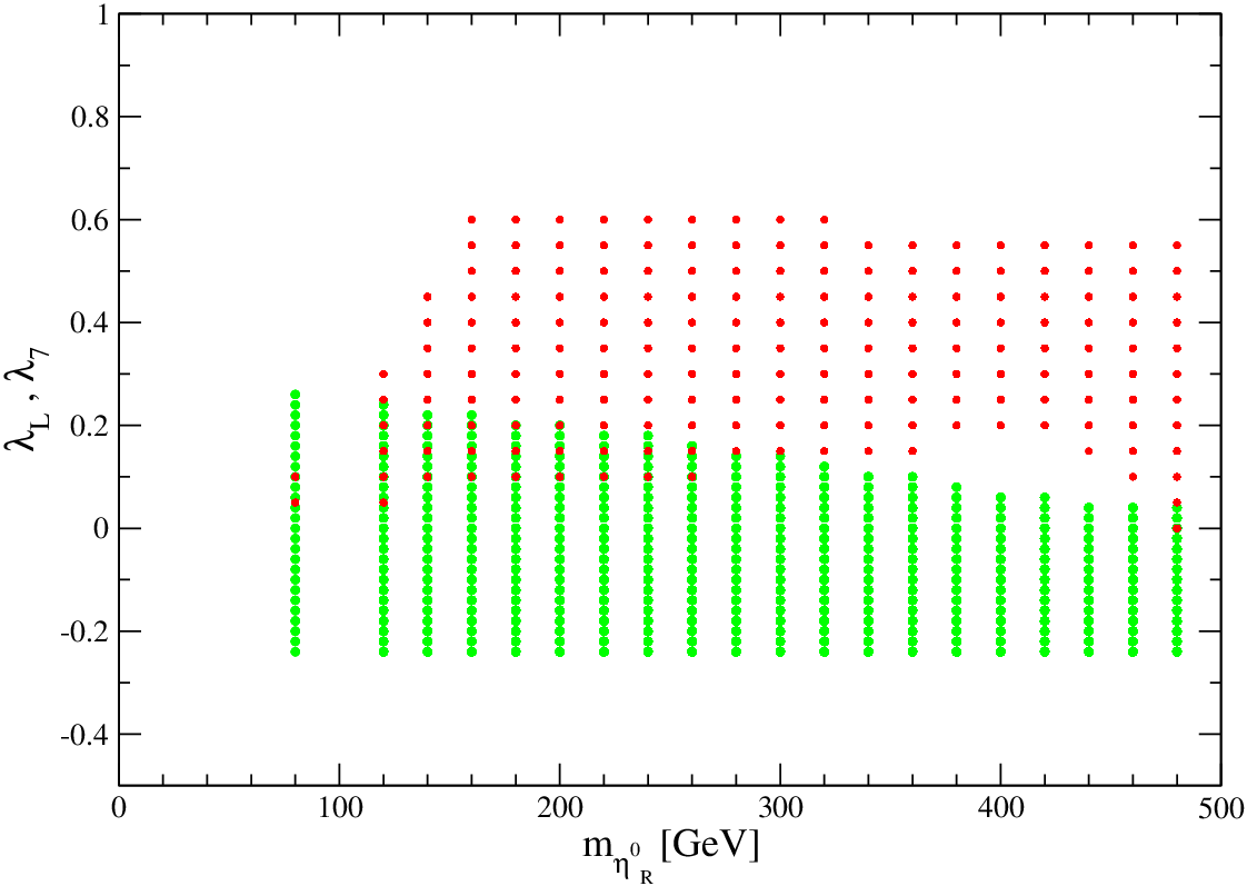
The presence of $\chi$ and $\phi$ changes the situation. Firstly, the separation of two allowed regions of $m_{\eta_{R}^{0}}$ disappears: As far as the relic abundance is concerned, $m_{\eta_{R}^{0}}$ is allowed between $80$ and $500$ GeV too, as we have seen, because $\chi$ and $\phi$ also contribute to the relic abundance. Secondly, the parameter space becomes considerably larger. To see how the allowed parameter space of the model without $\chi$ and $\phi$ changes, we consider a set of $(\delta_{1}=m_{\eta^{\pm}}-m_{\eta_{R}^{0}}~,~\delta_{2}=m_{\eta_{I}^{0}}-m_{\eta_{R}^{0}})$ , for which the allowed parameter space without $\chi$ and $\phi$ is very small. For $(\delta_{1}=10~,~\delta_{2}=10)$ GeV, for instance, there is no allowed range of $m_{\eta_{R}^{0}}\mathrel{\mathchoice{\vbox{\halign{$\m@th\displaystyle\hfil#\hfil$\cr<\crcr\sim\crcr}}}{\vbox{\halign{$\m@th\textstyle\hfil#\hfil$\cr<\crcr\sim\crcr}}}{\vbox{\halign{$\m@th\scriptstyle\hfil#\hfil$\cr<\crcr\sim\crcr}}}{\vbox{\halign{$\m@th\scriptscriptstyle\hfil#\hfil$\cr<\crcr\sim\crcr}}}}500$ GeV [43]; the low-mass range of $m_{\eta_{R}^{0}}$ , for which the relic abundance $\Omega_{\eta}h^{2}$ is consistent, does not satisfy the LEP constraint. Below we show how this situation changes in the presence of $\chi$ and $\phi$ . The LEP constraint implies that the region satisfying $m_{\eta_{R}^{0}}\mathrel{\mathchoice{\vbox{\halign{$\m@th\displaystyle\hfil#\hfil$\cr<\crcr\sim\crcr}}}{\vbox{\halign{$\m@th\textstyle\hfil#\hfil$\cr<\crcr\sim\crcr}}}{\vbox{\halign{$\m@th\scriptstyle\hfil#\hfil$\cr<\crcr\sim\crcr}}}{\vbox{\halign{$\m@th\scriptscriptstyle\hfil#\hfil$\cr<\crcr\sim\crcr}}}}80$ GeV and $m_{\eta_{I}^{0}}\mathrel{\mathchoice{\vbox{\halign{$\m@th\displaystyle\hfil#\hfil$\cr<\crcr\sim\crcr}}}{\vbox{\halign{$\m@th\textstyle\hfil#\hfil$\cr<\crcr\sim\crcr}}}{\vbox{\halign{$\m@th\scriptstyle\hfil#\hfil$\cr<\crcr\sim\crcr}}}{\vbox{\halign{$\m@th\scriptscriptstyle\hfil#\hfil$\cr<\crcr\sim\crcr}}}}100$ GeV with $\delta_{2}\mathrel{\mathchoice{\vbox{\halign{$\m@th\displaystyle\hfil#\hfil$\cr>\crcr\sim\crcr}}}{\vbox{\halign{$\m@th\textstyle\hfil#\hfil$\cr>\crcr\sim\crcr}}}{\vbox{\halign{$\m@th\scriptstyle\hfil#\hfil$\cr>\crcr\sim\crcr}}}{\vbox{\halign{$\m@th\scriptscriptstyle\hfil#\hfil$\cr>\crcr\sim\crcr}}}}8$ GeV is excluded [43]. Therefore, for $(\delta_{1}=10~,~\delta_{2}=10)$ GeV, we have to consider only $m_{\eta_{R}^{0}}>80$ GeV. Further, to suppress the parameter space, we assume that $m_{\chi}=m_{\eta_{R}^{0}}-10~\mbox{GeV}$ , $m_{\phi}=m_{\eta_{R}^{0}}-20~\mbox{GeV}$ , and $M_{k}=1000$ GeV, and we scan $m_{\eta_{R}^{0}}$ from $80$ to $500$ GeV.

Figure 9 shows the allowed area in the $\lambda_{L}(\lambda_{7})-m_{\eta_{R}^{0}}$ plane, where all the constraints are taken into account. The allowed mass range for $m_{\eta_{R}^{0}}$ is extended as expected. The reason that there are no allowed points around $m_{\eta_{R}^{0}}\simeq 100$ GeV is the following: Since we keep the mass difference fixed, we have $m_{\phi}=m_{\eta_{R}^{0}}-20\simeq 80$ GeV there. This is the threshold regime for the process $\phi\phi\to W^{+}W^{-}$ . So, for $m_{\eta_{R}^{0}}$ just below $100$ GeV, the annihilation cross section for $\phi$ is small because of small $\lambda_{7}$ in this range of $m_{\phi}$ , and therefore the relic abundance $\Omega_{\phi}h^{2}$ exceeds $0.12$ . We see that $m_{\eta_{R}^{0}}=80$ GeV is allowed, on the other hand. This allowed area exists, though $\lambda_{7}$ is small, because around $m_{\phi}=62$ GeV, the s-channel annihilation of $\phi$ becomes resonant due to $m_{h}=125$ GeV. For $m_{\eta_{R}^{0}}$ just above $100$ GeV, the annihilation cross section for $\phi$ is large because the channel to $W^{+}W^{-}$ is now open, so that $\Omega_{\phi}h^{2}$ cannot supplement the anyhow small $\Omega_{\eta}h^{2}$ .

If we suppress the constraint from the direct detection, we have a prediction on the direct detection. Figure 10 shows the spin-independent cross section off the nucleon versus the DM mass; the green (light gray) does so for the $\eta$ DM, and the violet (dark gray) area for the $\phi$ DM. We see that the the spin-independent cross sections not only are consistent with the current bound of XENON100 [63], but also are within the accessible range of future experiments.

III.3 Indirect detection

If DM annihilates sufficiently into SM particles, the resulting cosmic rays may be observable. These are indirect signals of DM, and in fact excesses in $e^{+}$ [73]–[76] and in $\gamma$ [77]–[80] have been recently reported. Indirect detection of DM has been studied within the framework of a two-component DM system in Refs. [8, 10, 13, 14, 15, 18, 26, 27], and also within the inert Higgs model in Refs. [42, 81, 83, 82]. As we see from the semi-annihilation diagram in Fig. 6, the process produces only a left-handed neutrino as the SM particle. Therefore, we are particularly interested in the neutrinos from the annihilation of captured DM in the Sun [44]–[53] (see Refs. [4, 5] for a review, and Refs. [83, 84] for the case of the inert Higgs model), because (i) the semi-annihilation produces a monochromatic neutrino ( $E_{\nu}\simeq m_{\eta^{0}_{R}}+m_{\phi}-m_{\chi}$ , for instance) in addition to those with $E_{\nu}\simeq m_{\eta^{0}_{R}}$ along with the continuum spectrum, (ii) these neutrinos can be observed at neutrino telescopes [86, 85, 87], and (iii) the evolution equations of the DM numbers in the Sun, which describe approaching equilibrium between the capture and annihilation (including conversion and semi-annihilation) rates of DM, are coupled now.

We denote the number of DM particles $\eta,\chi$ and $\phi$ in the Sun by $N_{i}$ , with $i=\eta,\chi$ and $\phi$ , respectively. Then the change of $N_{i}$ with respect to time $t$ is given by

$\displaystyle\dot{N}_{\eta}$	$\displaystyle=$	$\displaystyle C_{\eta}-C_{A}(\eta\eta\leftrightarrow\mbox{SM})N_{\eta}^{2}-C_{A}(\eta\eta\leftrightarrow\phi\phi)N_{\eta}^{2}-C_{A}(\eta\chi\leftrightarrow\phi\nu_{L})N_{\eta}N_{\chi}$	(65)
		$\displaystyle-C_{A}(\eta\phi\leftrightarrow\chi\nu_{L})N_{\eta}N_{\phi}+C_{A}(\phi\chi\leftrightarrow\eta\nu_{L})N_{\chi}N_{\phi}~,$	(65)
$\displaystyle\dot{N}_{\chi}$	$\displaystyle=$	$\displaystyle C_{\chi}-C_{A}(\chi\chi\leftrightarrow\phi\phi)N_{\chi}^{2}-C_{A}(\eta\chi\leftrightarrow\phi\nu_{L})N_{\eta}N_{\chi}$	(66)
		$\displaystyle+C_{A}(\eta\phi\leftrightarrow\chi\nu_{L})N_{\eta}N_{\phi}-C_{A}(\phi\chi\leftrightarrow\eta\nu_{L})N_{\chi}N_{\phi}~,$	(66)
$\displaystyle\dot{N}_{\phi}$	$\displaystyle=$	$\displaystyle C_{\phi}-C_{A}(\phi\phi\leftrightarrow\mbox{SM})N_{\phi}^{2}+C_{A}(\eta\eta\leftrightarrow\phi\phi)N_{\eta}^{2}+C_{A}(\chi\chi\leftrightarrow\phi\phi)N_{\chi}^{2}$	(67)
		$\displaystyle+C_{A}(\eta\chi\leftrightarrow\phi\nu_{L})N_{\eta}N_{\chi}-C_{A}(\eta\phi\leftrightarrow\chi\nu_{L})N_{\eta}N_{\phi}-C_{A}(\phi\chi\leftrightarrow\eta\nu_{L})N_{\chi}N_{\phi}~,$	(67)

where the $C_{i}$ ’s are the capture rates in the Sun, and the $C_{A}$ ’s are proportional to the annihilation cross sections times the relative DM velocity per volume in the limit $v\to 0$ :

	$\displaystyle C_{\phi(\eta)}$	$\displaystyle\simeq$	$\displaystyle 1.4\times 10^{20}f(m_{\phi(\eta_{R}^{0})})\left(\frac{\hat{f}}{0.3}\right)^{2}\left(\frac{\lambda_{7(L)}}{0.1}\right)^{2}\left[\frac{m_{h}}{125~\mbox{GeV}}\right]^{-4}$		(68)
		$\displaystyle\times$	$\displaystyle\left(\frac{200~\mbox{GeV}}{m_{\phi(\eta_{R}^{0})}}\right)^{2}\left(\frac{\Omega_{\phi(\eta)}h^{2}}{0.112}\right)\mbox{s}^{-1}~,~C_{\chi}=0~,$		(68)

where the function $f(m_{\phi(\eta_{R}^{0})})$ depends on the form factor of the nucleus, elemental abundance, kinematic suppression of the capture rate, etc., varying from $O(1)$ to $O(0.01)$ depending on the DM mass [50, 51]. The annihilation rates, $C_{A}$ , can be calculated from [48]

\displaystyle C_{A}(ij\leftrightarrow\bullet)

\displaystyle=

\displaystyle\frac{<\sigma(ij;\bullet)v>}{V_{ij}}~,~V_{ij}=5.7\times 10^{27}\left(\frac{100~\mbox{GeV}}{\mu_{ij}}\right)^{3/2}\mbox{cm}^{3}\,,

(69)

with $\mu_{ij}=2m_{i}m_{j}/(m_{i}+m_{j})$ in the limit $v\to 0$ .

There are fixed points of the evolution equations which correspond to equilibrium. Since at the time of the sun’s birth the numbers $N_{i}$ were zero, the $N_{i}$ ’s increase with time and approach the fixed-point values, i.e., equilibrium, at which point $N_{i}$ assumes its maximal value. So, the question is whether the age of the Sun, $t_{\odot}\simeq 4.5\times 10^{9}$ years, is old enough for $N_{i}$ to reach equilibrium. We see from the evolution equations that the fixed-point values are roughly proportional to $(C_{i}/C_{A})^{1/2}$ , implying that we need large capture rates $C_{i}$ to obtain large $N_{i}(t_{\odot})$ . The annihilation, conversion and semi-annihilation rates at $t=t_{\odot}$ are given by

\displaystyle\Gamma(ij;\bullet)

\displaystyle=

\displaystyle d_{ij}C_{A}(ij\leftrightarrow\bullet)N_{i}(t_{\odot})N_{j}(t_{\odot})~,

(70)

where $d_{ii}=1/2$ and $d_{ij}=1$ for $i\neq j$ . The observation rate of the neutrinos, $\Gamma_{\rm detect}$ , is proportional to $\Gamma(ij;\bullet)$ . As a benchmark, we use the same set of the input parameter values as in Eq. (52). In Fig. 11, we show the time evolution of¹⁰¹⁰ 10 For the monochromatic neutrinos, i.e. $\Gamma(\nu)$ , we have added all the semi-annihilations, because for the mass values given in Eq. (52) the neutrino energies are all close to $200$ GeV. Moreover, the first term in the r.h.s. of Eq. (72) (which counts neutrinos of $m_{\eta_{R}^{0}}+m_{\phi}-m_{\chi}=190$ GeV) is a dominant contribution with about $95$ %.

$\displaystyle\Gamma(\mbox{SM})$	$\displaystyle=$	$\displaystyle C_{A}(\eta\eta\leftrightarrow\mbox{SM})N_{\eta}^{2}/2+C_{A}(\phi\phi\leftrightarrow\mbox{SM})N_{\phi}^{2}/2~,$	(71)
$\displaystyle\Gamma(\nu)$	$\displaystyle=$	$\displaystyle C_{A}(\eta\phi\leftrightarrow\chi\nu)N_{\eta}N_{\phi}+C_{A}(\eta\chi\leftrightarrow\phi\nu)N_{\eta}N_{\chi}+C_{A}(\chi\phi\leftrightarrow\eta\nu)N_{\chi}N_{\phi}~,$	(72)
$\displaystyle\Gamma(\nu\nu)$	$\displaystyle=$	$\displaystyle C_{A}(\eta\eta\leftrightarrow\nu\nu)N_{\eta}^{2}/2~,$	(73)

scaled to $10^{20}~\mbox{s}^{-1}$ , as function of $\tau=t/t_{\odot}$ . As we see from Fig. 11, the rates seem to be saturated: $\Gamma(\mbox{SM})$ is in fact saturated, but $\Gamma(\nu)$ does not reach its fixed-point value of $0.002\times 10^{20}~\mbox{s}^{-1}$ at $\tau=t/t_{\odot}=1$ . The saturated value of $\Gamma(\mbox{SM})$ is $0.28\times 10^{20}~\mbox{s}^{-1}$ for the input parameters of Eq. (52), which is consistent with the upper limit of $\sim 2.73\times 10^{21}~\mbox{s}^{-1}$ for $m_{\rm DM}=250~\mbox{GeV}$ of the AMANDA-II / IceCube neutrino telescope [85]. As for the monochromatic neutrinos, we obtain $\Gamma(\nu)=1.1\times 10^{-3}\times 10^{20}~\mbox{s}^{-1}$ and $\Gamma(\nu\nu)=1.3\times 10^{-7}\times 10^{20}~\mbox{s}^{-1}$ . To estimate the detection rate $\Gamma_{\rm detect}$ , we use the formula [88]

\displaystyle\Gamma_{\rm detect}=AP(E_{\nu})\Gamma_{\rm inc}~,

(74)

where $A$ is the detector area facing the incident beam, $P(E_{\nu})$ is the probability for detection as a function of the neutrino energy $E_{\nu}$ , and $\Gamma_{\rm inc}=\Gamma/4\pi R_{\odot}^{2}$ is the incoming neutrino flux — i.e., the number of neutrinos per unit area per second on the Earth (where $R_{\odot}$ is the distance to the Sun $\simeq 1.5\times 10^{8}$ km).¹¹¹¹ 11 A sophisticated method to compute the observation rates at IceCube was recently developed in [89]. The probability $P(E_{\nu})$ may be approximated as the ratio of the effective detector length $L$ to the mean free path of the neutrinos in the detector. For the neutrinos (anti-neutrinos), one finds $P(E_{\nu(\bar{\nu})})\simeq 2.0(1.0)\times 10^{-11}(L/\mbox{km})(E_{\nu(\bar{\nu})}/\mbox{GeV})$ , arriving at

\displaystyle\Gamma_{\rm detect}

\displaystyle\simeq

\displaystyle 2.2(1.1)\times 10^{-21}\left(\frac{A}{\mbox{km}^{2}}\right)\left(\frac{L}{\mbox{km}}\right)\left(\frac{E_{\nu(\bar{\nu})}}{\mbox{GeV}}\right)~\left(\frac{\Gamma}{\mbox{s}^{-1}}\right)~\mbox{yr}^{-1}~,

(75)

which implies that, for the input parameters of Eq. (52), $0.05$ events of monochromatic neutrinos with $\sim 200$ GeV per year may be detected at IceCube [85], where we have used $A=1\mbox{km}^{2}$ , $L=1\mbox{km}$ .

A total of $0.05$ events per year may be too small to be realistic. However, we would like to note that we have studied only one point in the whole parameter space. It will be our future program to implement the sophisticated method of Ref. [89] and to survey the whole parameter space. How to observe the monochromatic neutrinos at neutrino telescopes should also be addressed [90]. Finally, we would like to note that if at least one of the fermionic DM particles in a multi-component DM system has odd parity of the discrete lepton number, then a monochromatic left-handed neutrino, which is also odd, can be produced together with this fermionic DM in a semi-annihilation of DM particles.

IV Conclusion

We have considered the conversion and semi-annihilation of DM in a multi-component DM system. We have found in fictive models that these non-standard DM annihilation processes can influence the relic abundance of DM a lot, which has been recently found for two-component DM systems in Refs. [17, 22, 23].

As a concrete three-component DM system, we have considered a radiative seesaw model of Ref. [32], which is extended to include an extra Majorana fermion $\chi$ and an extra real scalar boson $\phi$ . The DM stabilizing symmetry is promoted to $Z_{2}\times Z^{\prime}_{2}$ , and we have assumed that $\eta_{R}^{0}$ (the CP-even neutral component of the inert Higgs $SU(2)_{L}$ doublet), $\chi$ and $\phi$ are DM. We have shown that the previously found separation [41, 42, 43] of the allowed parameter space in the low- and high-mass regions for $\eta_{R}^{0}$ disappears in the presence of $\chi$ and $\phi$ .

Finally, we have discussed neutrinos coming from the annihilations of the captured DM in the Sun. The evolution equations of the DM numbers in the Sun, which describe approaching equilibrium between the capture and annihilation (including conversion and semi-annihilation) rates of DM, are coupled in a multi-component DM system. Due to the semi-annihilations of DM, monochromatic neutrinos are radiated, and the observation rates of neutrinos have been estimated. Observations of high-energy monochromatic neutrinos from the Sun may indicate a multi-component DM system.

The work of M. D. is supported by the International Max Planck Research School for Precision Tests of Fundamental Symmetries. The work of M. A. is supported in part by Grant-in-Aid for Scientific Research for Young Scientists (B) (Grant No.22740137), and J. K. is partially supported by Grant-in-Aid for Scientific Research (C) from Japan Society for Promotion of Science (Grant No.22540271). M. D. thanks the Institute for Theoretical Physics at Kanazawa University for very kind hospitality.

References

[1] A. G. Riess et al. [Supernova Search Team Collaboration], “Observational Evidence from Supernovae for an Accelerating Universe and a Cosmological Constant,” Astron. J. 116 (1998) 1009 [arXiv:astro-ph/9805201].
[2] K. N. Abazajian et al. [SDSS Collaboration], “The Seventh Data Release of the Sloan Digital Sky Survey,” Astrophys. J. Suppl. 182 (2009) 543 [arXiv:0812.0649 [astro-ph]].
[3] E. Komatsu et al. [WMAP Collaboration], “Seven-Year Wilkinson Microwave Anisotropy Probe (WMAP) Observations: Cosmological Interpretation,” Astrophys. J. Suppl. 192 (2011) 18 [arXiv:1001.4538 [astro-ph.CO]].
[4] G. Jungman, M. Kamionkowski, K. Griest, “Supersymmetric dark matter,” Phys. Rept. 267 (1996) 195-373 [arXiv:hep-ph/9506380].
[5] G. Bertone, D. Hooper and J. Silk, “Particle dark matter: Evidence, candidates and constraints,” Phys. Rept. 405 (2005) 279 [arXiv:hep-ph/0404175]; G. Bertone, (ed.), “Particle dark matter: Observations, models and searches,” Cambridge University Press 2010.
[6] M. Cirelli, “Indirect Searches for Dark Matter: a status review,” arXiv:1202.1454 [hep-ph].
[7] Z. G. Berezhiani and M. Y. .Khlopov, “Physics of cosmological dark matter in the theory of broken family symmetry,” Sov. J. Nucl. Phys. 52 (1990) 60 [Yad. Fiz. 52 (1990) 96]; Z. G. Berezhiani and M. Y. .Khlopov, “Cosmology of Spontaneously Broken Gauge Family Symmetry,” Z. Phys. C 49 (1991) 73.
[8] C. Boehm, P. Fayet, J. Silk, “Light and heavy dark matter particles,” Phys. Rev. D69 (2004) 101302 [arXiv:hep-ph/0311143].
[9] T. Hur, H.-S. Lee and S. Nasri, “A Supersymmetric U(1)-prime Model with Multiple Dark Matters,” Phys. Rev. D 77 (2008) 015008 [arXiv:0710.2653 [hep-ph]].
[10] Q. H. Cao, E. Ma, J. Wudka and C. P. Yuan, “Multipartite dark matter,” arXiv:0711.3881 [hep-ph].
[11] J. L. Feng and J. Kumar, “The WIMPless Miracle: Dark-Matter Particles without Weak-Scale Masses or Weak Interactions,” Phys. Rev. Lett. 101 (2008) 231301 [arXiv:0803.4196 [hep-ph]].
[12] H. S. Cheon, S. K. Kang and C. S. Kim, “Doubly Coexisting Dark Matter Candidates in an Extended Seesaw Model,” Phys. Lett. B 675 (2009) 203 [Erratum-ibid. B 698 (2011) 324] [arXiv:0807.0981 [hep-ph]].
[13] J.-H. Huh, J. E. Kim, B. Kyae, “Two dark matter components in dark matter extension of the minimal supersymmetric standard model and the high energy positron spectrum in PAMELA/HEAT data,” Phys. Rev. D79 (2009) 063529 [arXiv:0809.2601 [hep-ph]].
[14] M. Fairbairn and J. Zupan, “Dark matter with a late decaying dark partner,” JCAP 0907 (2009) 001 [arXiv:0810.4147 [hep-ph]].
[15] K. M. Zurek, “Multi-Component Dark Matter,” Phys. Rev. D79 (2009) 115002 [arXiv:0811.4429 [hep-ph]].
[16] D. E. Morrissey, D. Poland and K. M. Zurek, “Abelian Hidden Sectors at a GeV,” JHEP 0907 (2009) 050 [arXiv:0904.2567 [hep-ph]].
[17] F. D’Eramo and J. Thaler, “Semi-annihilation of Dark Matter,” JHEP 1006 (2010) 109 [arXiv:1003.5912 [hep-ph]].
[18] D. Feldman, Z. Liu, P. Nath and G. Peim, “Multicomponent Dark Matter in Supersymmetric Hidden Sector Extensions,” Phys. Rev. D 81 (2010) 095017 [arXiv:1004.0649 [hep-ph]].
[19] B. Batell, “Dark Discrete Gauge Symmetries,” Phys. Rev. D 83 (2011) 035006 [arXiv:1007.0045 [hep-ph]].
[20] Z.-P. Liu, Y.-L. Wu and Y.-F. Zhou, “Enhancement of dark matter relic density from the late time dark matter conversions,” Eur. Phys. J. C 71 (2011) 1749 [arXiv:1101.4148 [hep-ph]].
[21] K. R. Dienes and B. Thomas, “Dynamical Dark Matter: I. Theoretical Overview,” Phys. Rev. D 85 (2012) 083523 [arXiv:1106.4546 [hep-ph]]; K. R. Dienes and B. Thomas, “Dynamical Dark Matter: II. An Explicit Model,” Phys. Rev. D 85 (2012) 083524 [arXiv:1107.0721 [hep-ph]]; K. R. Dienes, S. Su and B. Thomas, “Distinguishing Dynamical Dark Matter at the LHC,” arXiv:1204.4183 [hep-ph].
[22] G. Belanger and J.-C. Park, “Assisted freeze-out,” JCAP 1203 (2012) 038 [arXiv:1112.4491 [hep-ph]].
[23] G. Belanger, K. Kannike, A. Pukhov and M. Raidal, “Impact of semi-annihilations on dark matter phenomenology - an example of $Z_{N}$ symmetric scalar dark matter,” JCAP 1204 (2012) 010 [arXiv:1202.2962 [hep-ph]].
[24] I. P. Ivanov and V. Keus, “ $Z_{p}$ scalar dark matter from multi-Higgs-doublet models,” arXiv:1203.3426 [hep-ph].
[25] E. Ma, “Supersymmetric Model of Radiative Seesaw Majorana Neutrino Masses,” Annales Fond. Broglie 31 (2006) 285 [arXiv:hep-ph/0607142]; E. Ma, “Supersymmetric U(1) Gauge Realization of the Dark Scalar Doublet Model of Radiative Neutrino Mass,” Mod. Phys. Lett. A23 (2008) 721 [arXiv:0801.2545 [hep-ph]].
[26] H. Fukuoka, J. Kubo and D. Suematsu, “Anomaly Induced Dark Matter Decay and PAMELA/ATIC Experiments,” Phys. Lett. B 678 (2009) 401 [arXiv:0905.2847 [hep-ph]].
[27] H. Fukuoka, D. Suematsu and T. Toma, “Signals of dark matter in a supersymmetric two dark matter model,” JCAP 1107 (2011) 001 [arXiv:1012.4007 [hep-ph]].
[28] D. Suematsu and T. Toma, “Dark matter in the supersymmetric radiative seesaw model with an anomalous U(1) symmetry,” Nucl. Phys. B 847 (2011) 567 [arXiv:1011.2839 [hep-ph]].
[29] M. Aoki, J. Kubo, T. Okawa and H. Takano, “Impact of Inert Higgsino Dark Matter,” Phys. Lett. B 707 (2012) 107 [arXiv:1110.5403 [hep-ph]].
[30] E. Ma, “Z(3) Dark Matter and Two-Loop Neutrino Mass,” Phys. Lett. B 662 (2008) 49 [arXiv:0708.3371 [hep-ph]].
[31] K. Agashe, D. Kim, M. Toharia and D. G. E. Walker, “Distinguishing Dark Matter Stabilization Symmetries Using Multiple Kinematic Edges and Cusps,” Phys. Rev. D 82 (2010) 015007 [arXiv:1003.0899 [hep-ph]].
[32] E. Ma, “Verifiable radiative seesaw mechanism of neutrino mass and dark matter,” Phys. Rev. D 73 (2006) 077301 [arXiv:hep-ph/0601225].
[33] K. Griest, “Cross-Sections, Relic Abundance and Detection Rates for Neutralino Dark Matter,” Phys. Rev. D 38 (1988) 2357 [Erratum-ibid. D 39 (1989) 3802].
[34] M. Srednicki, R. Watkins and K. A. Olive, “Calculations of Relic Densities in the Early Universe,” Nucl. Phys. B 310 (1988) 693.
[35] K. Griest, M. Kamionkowski and M. S. Turner, “Supersymmetric Dark Matter Above the W Mass,” Phys. Rev. D 41 (1990) 3565.
[36] E. W. Kolb and M. S. Turner, “The Early Universe,” Front. Phys. 69 (1990) 1.
[37] P. Gondolo and G. Gelmini, “Cosmic abundances of stable particles: Improved analysis,” Nucl. Phys. B 360 (1991) 145.
[38] M. Drees, M. M. Nojiri, “The Neutralino relic density in minimal $N=1$ supergravity,” Phys. Rev. D47 (1993) 376-408 [arXiv:hep-ph/9207234].
[39] K. Griest, D. Seckel, “Three exceptions in the calculation of relic abundances,” Phys. Rev. D43 (1991) 3191-3203.
[40] J. R. Ellis, T. Falk and K. A. Olive, “Neutralino - Stau coannihilation and the cosmological upper limit on the mass of the lightest supersymmetric particle,” Phys. Lett. B 444 (1998) 367 [arXiv:hep-ph/9810360]; J. R. Ellis, T. Falk, K. A. Olive and M. Srednicki, “Calculations of neutralino-stau coannihilation channels and the cosmologically relevant region of MSSM parameter space,” Astropart. Phys. 13 (2000) 181 [Erratum-ibid. 15 (2001) 413] [arXiv:hep-ph/9905481].
[41] R. Barbieri, L. J. Hall and V. S. Rychkov, “Improved naturalness with a heavy Higgs: An alternative road to LHC physics,” Phys. Rev. D 74 (2006) 015007 [arXiv:hep-ph/0603188].
[42] L. Lopez Honorez, E. Nezri, J. F. Oliver and M. H. G. Tytgat, “The Inert Doublet Model: An Archetype for Dark Matter,” JCAP 0702 (2007) 028 [arXiv:hep-ph/0612275].
[43] E. M. Dolle and S. Su, “The Inert Dark Matter,” Phys. Rev. D 80 (2009) 055012 [arXiv:0906.1609 [hep-ph]].
[44] J. Silk, K. A. Olive and M. Srednicki, “The Photino, the Sun and High-Energy Neutrinos,” Phys. Rev. Lett. 55 (1985) 257.
[45] L. M. Krauss, M. Srednicki and F. Wilczek, “Solar System Constraints and Signatures for Dark Matter Candidates,” Phys. Rev. D 33 (1986) 2079.
[46] K. Freese, “Can Scalar Neutrinos or Massive Dirac Neutrinos Be the Missing Mass?,” Phys. Lett. B 167 (1986) 295.
[47] T. K. Gaisser, G. Steigman and S. Tilav, “Limits on Cold Dark Matter Candidates from Deep Underground Detectors,” Phys. Rev. D 34 (1986) 2206.
[48] K. Griest and D. Seckel, “Cosmic Asymmetry, Neutrinos and the Sun,” Nucl. Phys. B 283 (1987) 681 [Erratum-ibid. B 296 (1988) 1034].
[49] S. Ritz and D. Seckel, “Detailed Neutrino Spectra From Cold Dark Matter Annihilations In The Sun,” Nucl. Phys. B 304 (1988) 877.
[50] M. Kamionkowski, “Energetic neutrinos from heavy neutralino annihilation in the sun,” Phys. Rev. D 44 (1991) 3021.
[51] M. Kamionkowski, K. Griest, G. Jungman and B. Sadoulet, “Model independent comparison of direct versus indirect detection of supersymmetric dark matter,” Phys. Rev. Lett. 74 (1995) 5174 [arXiv:hep-ph/9412213].
[52] H.-C. Cheng, J. L. Feng and K. T. Matchev, “Kaluza-Klein dark matter,” Phys. Rev. Lett. 89 (2002) 211301 [arXiv:hep-ph/0207125].
[53] D. Hooper and G. D. Kribs, “Probing Kaluza-Klein dark matter with neutrino telescopes,” Phys. Rev. D 67 (2003) 055003 [arXiv:hep-ph/0208261].
[54] E. Ma and M. Raidal, “Neutrino mass, muon anomalous magnetic moment, and lepton flavor nonconservation,” Phys. Rev. Lett. 87 (2001) 011802 [Erratum-ibid. 87 (2001) 159901] [arXiv:hep-ph/0102255].
[55] K. Hayasaka, “Recent Tau Decay Results at B Factories -Lepton Flavor Violating Tau Decays,” arXiv:1010.3746 [hep-ex].
[56] K. Nakamura et al. [Particle Data Group Collaboration], “Review of particle physics,” J. Phys. G G 37 (2010) 075021 and 2011 partial update for the 2012 edition.
[57] M. Gustafsson, S. Rydbeck, L. Lopez-Honorez and E. Lundstrom, “Status of the Inert Doublet Model and the Role of multileptons at the LHC,” arXiv:1206.6316 [hep-ph].
[58] E. Dolle, X. Miao, S. Su and B. Thomas, “Dilepton Signals in the Inert Doublet Model,” Phys. Rev. D 81 (2010) 035003 [arXiv:0909.3094 [hep-ph]];
[59] M. Cirelli, N. Fornengo and A. Strumia, “Minimal dark matter,” Nucl. Phys. B 753 (2006) 178 [arXiv:hep-ph/0512090].
[60] D. Schmidt, T. Schwetz and T. Toma, “Direct Detection of Leptophilic Dark Matter in a Model with Radiative Neutrino Masses,” Phys. Rev. D 85 (2012) 073009 [arXiv:1201.0906 [hep-ph]].
[61] J. R. Ellis, A. Ferstl and K. A. Olive, “Reevaluation of the elastic scattering of supersymmetric dark matter,” Phys. Lett. B 481 (2000) 304 [arXiv:hep-ph/0001005].
[62] L. L. Honorez and C. E. Yaguna, “A new viable region of the inert doublet model,” JCAP 1101 (2011) 002 [arXiv:1011.1411 [hep-ph]].
[63] E. Aprile et al. [XENON100 Collaboration], “Dark Matter Results from 100 Live Days of XENON100 Data,” Phys. Rev. Lett. 107 (2011) 131302 [arXiv:1104.2549 [astro-ph.CO]].
[64] G. Angloher, M. Bauer, I. Bavykina, A. Bento, A. Brown, C. Bucci, C. Ciemniak, C. Coppi, G. Deuter, F. von Feilitzsch et al., “Commissioning Run of the CRESST-II Dark Matter Search,” arXiv:0809.1829 [astro-ph].
[65] V. N. Lebedenko, H. M. Araujo, E. J. Barnes, A. Bewick, R. Cashmore, V. Chepel, A. Currie and D. Davidge et al., “Result from the First Science Run of the ZEPLIN-III Dark Matter Search Experiment,” Phys. Rev. D 80 (2009) 052010 [arXiv:0812.1150 [astro-ph]].
[66] Z. Ahmed et al. [The CDMS-II Collaboration], “Dark Matter Search Results from the CDMS II Experiment,” Science 327 (2010) 1619 [arXiv:0912.3592 [astro-ph.CO]].
[67] C. E. Aalseth et al. [CoGeNT Collaboration], “Results from a Search for Light-Mass Dark Matter with a P-type Point Contact Germanium Detector,” Phys. Rev. Lett. 106 (2011) 131301 [arXiv:1002.4703 [astro-ph.CO]].
[68] R. Bernabei et al. [DAMA and LIBRA Collaborations], “New results from DAMA/LIBRA,” Eur. Phys. J. C 67 (2010) 39 [arXiv:1002.1028 [astro-ph.GA]].
[69] S. C. Kim, H. Bhang, J. H. Choi, W. G. Kang, B. H. Kim, H. J. Kim, K. W. Kim and S. K. Kim et al., “New Limits on Interactions between Weakly Interacting Massive Particles and Nucleons Obtained with CsI(Tl) Crystal Detectors,” arXiv:1204.2646 [astro-ph.CO].
[70] T. Bruch [CDMS Collaboration], “CDMS-II to SuperCDMS: WIMP search at a zeptobarn,” arXiv:1001.3037 [astro-ph.IM].
[71] M. Selvi [XENON1T Collaboration], “Study of the performances of the shield and muon veto of the XENON1T experiment,” PoS IDM 2010 (2011) 053.
[72] H. Sekiya, “Xmass,” J. Phys. Conf. Ser. 308 (2011) 012011 [arXiv:1006.1473 [astro-ph.IM]].
[73] O. Adriani et al. [PAMELA Collaboration], “An anomalous positron abundance in cosmic rays with energies 1.5-100 GeV,” Nature 458 (2009) 607 [arXiv:0810.4995 [astro-ph]].
[74] S. W. Barwick et al. [HEAT Collaboration], “Measurements of the cosmic ray positron fraction from 1-GeV to 50-GeV,” Astrophys. J. 482 (1997) L191 [arXiv:astro-ph/9703192].
[75] M. Aguilar et al. [AMS-01 Collaboration], “Cosmic-ray positron fraction measurement from 1 to 30-GeV with AMS-01,” Phys. Lett. B 646 (2007) 145 [arXiv:astro-ph/0703154].
[76] M. Ackermann et al. [The Fermi LAT Collaboration], “Measurement of separate cosmic-ray electron and positron spectra with the Fermi Large Area Telescope,” Phys. Rev. Lett. 108 (2012) 011103 [arXiv:1109.0521 [astro-ph.HE]].
[77] F. Aharonian et al. [HESS Collaboration], “Very high-energy gamma rays from the direction of Sagittarius A*,” Astron. Astrophys. 425 (2004) L13 [arXiv:astro-ph/0408145]; F. Aharonian et al. [H.E.S.S. Collaboration], “H.E.S.S. observations of the Galactic Center region and their possible dark matter interpretation,” Phys. Rev. Lett. 97 (2006) 221102 [Erratum-ibid. 97 (2006) 249901] [arXiv:astro-ph/0610509].
[78] W. B. Atwood et al. [LAT Collaboration], “The Large Area Telescope on the Fermi Gamma-ray Space Telescope Mission,” Astrophys. J. 697 (2009) 1071 [arXiv:0902.1089 [astro-ph.IM]].
[79] J. Aleksic et al. [MAGIC Collaboration], “MAGIC Gamma-Ray Telescope Observation of the Perseus Cluster of Galaxies: Implications for Cosmic Rays, Dark Matter and NGC 1275,” Astrophys. J. 710 (2010) 634 [arXiv:0909.3267 [astro-ph.HE]].
[80] V. A. Acciari et al. [VERITAS Collaboration], “VERITAS Search for VHE Gamma-ray Emission from Dwarf Spheroidal Galaxies,” Astrophys. J. 720 (2010) 1174 [arXiv:1006.5955 [astro-ph.CO]].
[81] M. Gustafsson, E. Lundstrom, L. Bergstrom and J. Edsjo, “Significant Gamma Lines from Inert Higgs Dark Matter,” Phys. Rev. Lett. 99 (2007) 041301 [arXiv:astro-ph/0703512].
[82] D. Suematsu, T. Toma and T. Yoshida, “Enhancement of the annihilation of dark matter in a radiative seesaw model,” Phys. Rev. D 82 (2010) 013012 [arXiv:1002.3225 [hep-ph]].
[83] P. Agrawal, E. M. Dolle and C. A. Krenke, “Signals of Inert Doublet Dark Matter in Neutrino Telescopes,” Phys. Rev. D 79 (2009) 015015 [arXiv:0811.1798 [hep-ph]].
[84] S. Andreas, M. H. G. Tytgat and Q. Swillens, “Neutrinos from Inert Doublet Dark Matter,” JCAP 0904 (2009) 004 [arXiv:0901.1750 [hep-ph]].
[85] R. Abbasi et al. [IceCube Collaboration], “Multi-year search for dark matter annihilations in the Sun with the AMANDA-II and IceCube detectors,” Phys. Rev. D 85 (2012) 042002 [arXiv:1112.1840 [astro-ph.HE]].
[86] T. Tanaka et al. [Super-Kamiokande Collaboration], “An Indirect Search for WIMPs in the Sun using 3109.6 days of upward-going muons in Super-Kamiokande,” Astrophys. J. 742 (2011) 78 [arXiv:1108.3384 [astro-ph.HE]].
[87] J. D. Zornoza, “Dark matter search with the ANTARES neutrino telescope,” arXiv:1204.5066 [astro-ph.HE].
[88] F. Halzen and S. R. Klein, “IceCube: An Instrument for Neutrino Astronomy,” Rev. Sci. Instrum. 81 (2010) 081101 [arXiv:1007.1247 [astro-ph.HE]].
[89] P. Scott et al. [the IceCube Collaboration], “Use of event-level neutrino telescope data in global fits for theories of new physics,” arXiv:1207.0810 [hep-ph].
[90] A. Esmaili and Y. Farzan, “On the Oscillation of Neutrinos Produced by the Annihilation of Dark Matter inside the Sun,” Phys. Rev. D 81 (2010) 113010 [arXiv:0912.4033 [hep-ph]]; “A Novel Method to Extract Dark Matter Parameters from Neutrino Telescope Data,” JCAP 1104 (2011) 007 [arXiv:1011.0500 [hep-ph]].

	$\displaystyle-(\mbox{PSI})\|M(ii;X_{i}X^{\prime}_{i})\|^{2}\frac{\bar{f}_{i}\bar{f}_{i}}{\bar{n}_{i}\bar{n}_{i}}\left(n_{i}n_{i}-\bar{n}_{i}\bar{n}_{i}\right)$
	$\displaystyle-\sum_{i>j}(\mbox{PSI})~\|M(ii;jj)\|^{2}\frac{\bar{f}_{i}\bar{f}_{i}}{\bar{n}_{i}\bar{n}_{i}}\left(n_{i}n_{i}-\frac{n_{j}n_{j}}{\bar{n}_{j}\bar{n}_{j}}\bar{n}_{i}\bar{n}_{i}\right)$
	$\displaystyle+\sum_{j>i}(\mbox{PSI})~\|M(jj;ii)\|^{2}\frac{\bar{f}_{j}\bar{f}_{j}}{\bar{n}_{j}\bar{n}_{j}}\left(n_{j}n_{j}-\frac{n_{i}n_{i}}{\bar{n}_{i}\bar{n}_{i}}\bar{n}_{j}\bar{n}_{j}\right)$
	$\displaystyle-\sum_{j,k}(\mbox{PSI})~\|M(ij;kX_{ijk})\|^{2}\frac{\bar{f}_{i}\bar{f}_{j}}{\bar{n}_{i}\bar{n}_{j}}\left(n_{i}n_{j}-\frac{n_{k}}{\bar{n}_{k}}\bar{n}_{i}\bar{n}_{j}\right)$
	$\displaystyle+\sum_{j,k}(\mbox{PSI})~\|M(jk;iX_{jki})\|^{2}\frac{\bar{f}_{j}\bar{f}_{k}}{\bar{n}_{j}\bar{n}_{k}}\left(n_{j}n_{k}-\frac{n_{i}}{\bar{n}_{i}}\bar{n}_{j}\bar{n}_{k}\right)~,$		(6)

Multi-Component Dark Matter Systems and Their Observation Prospects