Constraints on coupled dark energy using CMB data from WMAP and SPT
Abstract
We consider the case of a coupling in the dark cosmological sector, where a dark energy scalar field modifies the gravitational attraction between dark matter particles. We find that the strength of the coupling is constrained using current Cosmic Microwave Background (CMB) data, including WMAP7 and SPT, to be less than 0.063 (0.11) at () confidence level. Further, we consider the additional effect of the CMB-lensing amplitude, curvature, effective number of relativistic species and massive neutrinos and show that the bound from current data on is already strong enough to be rather stable with respect to any of these variables. The strongest effect is obtained when we allow for massive neutrinos, in which case the bound becomes slightly weaker, . A larger value of the effective number of relativistic degrees of freedom favors larger couplings between dark matter and dark energy as well as values of the spectral index closer to . Adding the present constraints on the Hubble constant, as well as from baryon acoustic oscillations and supernovae Ia, we find . In this case we also find an interesting likelihood peak for (still compatible with 0 at 1). This peak comes mostly from a slight difference between the Hubble parameter HST result and the WMAP7+SPT best fit. Finally, we show that forecasts of Planck+SPT mock data can pin down the coupling to a precision of better than and detect whether the marginal peak we find at small non zero coupling is a real effect.
I Introduction
Cosmic Microwave Background (CMB) probes have recently broadened our knowledge of primordial acoustic oscillations to small angular scales, extending previous measurements of temperature power spectrum (Wilkinson Microwave Anisotropy Probe 7, [1]) up to with first compelling evidence of CMB lensing from the South Pole Telescope (SPT, [2]) and Atacama Cosmology Telescope (ACT, [3]). The impact of small-scale CMB measurements and gravitational lensing on cosmology is relevant [4] and can be used to constrain cosmological parameters and to address one of the major issues of present cosmology, that is to say the nature of dark energy [5, 6, 7, 8, 9, 10]. The simplest framework for dark energy models considers dark energy as a cosmological constant , contributing to about of the total energy density in the universe and providing late time cosmic acceleration, while a Cold Dark Matter represents about (CDM model). Though theoretically in good agreement with present observations, a cosmological constant is somewhat unpleaseantly affected by the coincidence and fine-tuning problems which seem unavoidable in such a framework. Many alternative models have been proposed, though it is fair to say that so far no one completely avoids these problems. Some encouraging arguments have been put forward in the framework of dynamical dark energy models, where a scalar field (quintessence or cosmon) rolls down a suitable potential [11, 12] possibly interacting with dark matter [13, 14] or gravity [15, 16] and therefore modifying the growth of structure. Usually, one of the features of such dynamical dark energy models is to have a non-negligible amount of dark energy at early times. The amount of early dark energy (early referring to the time of decoupling) influences CMB peaks in various ways and can be strongly constrained when including small scale measurements, as shown for instance in Refs. [17, 18].
In this paper, we consider the case of coupled dark energy models, in which dark matter particles feel an interaction, additional to gravity, mediated by the dark energy scalar field. Such an interaction introduces effectively a coupling between the evolution of the dark energy scalar field and dark matter particles. In this sense, this class of models is both an example in which a non-negligible amount of early dark energy is present as well as a typical scenario of modified gravity theories. When seen in the Jordan frame, a coupling between matter and dark energy can be reformulated in terms of scalar-tensor theories (or models). This is exactly true when the contribution of baryons is neglected. In the Einstein frame, it is common use to neglect a coupling to baryon within coupled dark energy models, and consider only dark energy - dark matter interactions. Alternatively, in the Jordan frame, scalar-tensor theories ( models) require some sort of screening mechanism (like chameleon [19, 20, 21, 22] or symmetrons [23]) that protects the dark energy scalar field and its mass within high density regions, so that local solar system constraints are satisfied.
The strength of the coupling affects CMB in several ways, changing the amplitude, the position of the peaks as well as contributing to the Late Integrated Sachs-Wolfe (ISW) effect (manifest at large length scales) and to gravitational lensing (appearing at small length scales in the temperature spectrum). Moreover, the coupling is degenerate with the amount of cold dark matter , the spectral index , the Hubble parameter (see [24] for a review). After recalling the effects of the coupling on CMB, we use a Monte Carlo analysis to constrain the coupling combining WMAP and SPT real data. Furthermore we extend our analysis to forecasting the constraints that Planck data are expected to put on the coupling parameter, combined with mock SPT data.
This paper is organized as follows. In Section II we recall the main features of coupled dark energy (CDE) cosmologies. In section III we recall effects of the coupling on the CMB spectrum and describe the methods used, both with regard to the implementation of the numerical code and the data used for this paper. In Section IV we derive the constraints from existing data for several different runs, including effects of the effective relativistic degree of freedom , CMB-lensing, curvature and massive neutrinos. Here we also forecast the constraining capability in presence of the forthcoming Planck data, joined with SPT mock data. Finally, in Section V we derive our conclusions.
II Coupled Dark Energy
We consider the case in which an interaction is present between dark energy and dark matter, as illustrated in [25, 13, 26, 27, 28, 14]. Such cosmologies have to be seen within the framework of modified gravity, since effectively the gravitational interaction perceived by dark matter particles is modified with respect to standard General Relativity. Coupled dark energy cosmologies considered here are described by the lagrangian:
| (1) |
in which the mass of matter fields is a function of the scalar field . We consider the case in which the DE is only coupled to CDM (hereafter denoted with a subscript , while the subscript will denote baryons). In this case, the coupling is not affected by tests on the equivalence principle and solar system constraints and can therefore be stronger than the one with baryons. The choice specifies the coupling and as a consequence the quantity via the expression:
| (2) |
acts as a source term in the Bianchi identities:
| (3) |
If no other species is involved in the coupling then . Various choices of couplings have been investigated in literature, including constant [29, 30, 31, 32, 33, 34, 35, 36, 37, 38] and varying couplings [39]. For a constant coupling, typical values of presently allowed by observations (within current CMB data) are within the range (at 95% CL for a constant coupling and an exponential potential) [27, 26, 28, 40], or possibly more [41, 42] if neutrinos are taken into account or for more realistic time-dependent choices of the coupling. Analysis of the models and constraint on these couplings have been obtained in several other ways, including spherical collapse ([43, 44] and references therein), higher-order expansions with the time renormalizazion group [45], -body simulations [46, 47, 39] and effects on supernovae, CMB and cross-correlation of CMB and LSS [27, 28, 40, 41, 42, 48, 49, 50, 51] together with Fisher matrix forecasts analysis combining power spectrum and Baryonic Acoustic Oscillations measurements as expected by the Euclid satellite 11 1 http://www.euclid-ec.org/ and http://sci.esa.int/euclid and CMB as expected from Planck [24].
The zero-component of equation (3) gives the conservation equations for the energy densities of each species:
| (4) | |||||
Here we have treated each component as a fluid with , where is the fluid 4-velocity and is the equation of state. Primes denote derivative with respect to conformal time . The class of models considered here corresponds to the choice:
| (5) |
with the coupling term equal to
| (6) |
Equivalently, the scalar field evolves according to the Klein-Gordon equation, which now includes an extra term that depends on CDM energy density:
| (7) |
Throughout this paper we choose an inverse power law potential defined as:
| (8) |
with and constants.
III The coupling effect on the CMB power spectrum
As discussed in [24], the coupling has two main effects on the CMB: 1) it shifts the position of the acoustic peaks to larger ’s due to the increase in the last scattering surface distance (sometimes called projection effect, [35] and references therein); 2) it reduces the ratio of baryons to dark matter at decoupling with respect to its present value, since coupled dark matter dilute faster than in an uncoupled model. Both effects are clearly visible in Fig. (1) for various values of .

In Fig.2 the effect of the coupling on the CMB is more evident. The figure shows the quantity (i.e. the usual TT spectrum plotted in Fig.(1) multiplied by ), as suggested for example in [53]. In Fig.2 we also show the effect of including CMB-lensing on the TT spectrum for the same value of the coupling constant: the unlensed TT spectrum (blue dot dashed) clearly differs from the corresponding lensed one (solid blue), an effect which is larger at small scales (large l). The position of the peaks remains invariant but the amplitude is larger and, for , the throats appear more pronounced than the peaks.


The purpose of our analysis is to use recent CMB observations reaching multipoles up to to constrain dynamical dark energy models in which a coupling is present between the quintessence scalar field (or cosmon, seen as the mediator of a fifth force between dark matter particles) and dark matter. In order to do so, we proceed as follows.
III.1 Theoretical spectra
Theoretical CMB and lensing power spectra have been produced using the code IDEA (Interacting Dark Energy Anisotropies) based on CAMB [54] and able to include dynamical dark energy, Early Dark Energy parameterizations (not included in this analysis) as well as interacting dark energy models. In order to include the coupling, both background and linear perturbations have been modified following Refs. [30, 35]. The output has been compared to an independent code [28] that is built on CMBFAST and the agreement was better than 1. The difficulty in the implementation relies on the fact that the initial conditions cannot be obtained analytically as in simple dark energy parameterizations (early dark energy or ): instead, they must be found by trial and error, through an iterative routine that finds the initial conditions required to get the desired present values of the cosmological parameters.
We have then performed a Monte Carlo analysis integrating IDEA within COSMOMC [55] comparing our theoretical predictions with the data presented in the next subsection.
We recall that the CMB coming from the last scattering surface (LSS) is bent by gravitational structures on the path towards us; this effect is called CMB-lensing [56, 4]. The standard deviation of the deflection angle is of the order of 2 arcminutes, which would correspond to small scales and multipoles, where CMB peaks are already damped by photon diffusion. However, deflection angles are correlated with each other over degree scales, so that lensing can have an important effect on the scales of the primary acoustic peaks, mainly smoothing them and transferring power to larger multipoles. Recently, CMB lensing detection has been claimed by several groups analyzing total intensity CMB anisotropies [3, 2].
CMB lensing is a probe of the expansion rate and naturally depends on the growth of perturbation and on the gravitational potentials; since dark energy affects both aspects, CMB lensing represents a way to discriminate among dynamical Dark Energy models and CDM, with promising results [5, 6, 7, 8, 9, 10]. In particular, the CMB weak lensing theory in generalized cosmologies has been outlined in [7]. The difference between the lensed and unlensed curves in Fig.1 shows the typical effects from CMB lensing. The acoustic peaks are smeared because of the correlation between different scales induced by lensing, and for the same reason a fraction of power is transferred to the angular domain corresponding to the damping tail, therefore dominating that part of the spectrum. Earlier works [8] have pointed out how the lensing is most relevant in particular in early dark energy models, as it injects power at the onset of cosmic acceleration, constraining the dark energy abundance in the corresponding epoch. On these lines, the analysis in [10] has shown that the inclusion of lensing data promote the CMB alone to be a probe of the existence of dark energy, breaking geometrical degeneracies associated to the pure CMB anisotropies at last scattering.
Also, the lensing depends on time, combining information from decoupling (from the last scattering surface of the CMB) and (when large scale structures formed); recent studies [57, 58] focus on implementing and investigating simulations of CMB lensing through cosmological structures in N-body simulations.
During matter dominated era (MDE), the potentials encountered along the way are constant in the linear regime and the gradient of the potential causes a total deflection angle given by:
| (9) |
where is the conformal distance of the source acting as a lens, is its gravitational potential, is the conformal time at which the CMB photon was at position .
One can also define the gravitational lensing potential
| (10) |
The lensed CMB temperature in a direction is given by the unlensed temperature in the deflected direction where at lowest order the deflection angle is just the gradient of the lensing potential. Expanding the lensing potential into spherical harmonics, one can define also the angular power spectrum corresponding to the lensing potential, defined as ; the latter (multiplied by ) is shown in Fig.2 (lower panel) for different values of the coupling. As we can see from the plot, the CMB lensing potential mainly gives contribution to large scales up to or less. However, the lensed CMB temperature power spectrum depends on the convolution between the lensing potential and the unlensed temperature spectrum (see [4] for more details) whose effect is of several percent at , thus being important when estimating the spectrum up to small scales of , as for the data we consider in the following.
III.2 Observed data
We have compared theoretical predictions of CMB lensed spectra with two datasets. The first includes WMAP7 temperature spectra [1]. The second includes the recently released power spectrum data from SPT [2]. Together with the ATC [3], SPT [2] has recently shown evidence of CMB-lensing with an enhancement in the CMB temperature power spectrum up to . We do not use ACT data in this analysis.
In order to use SPT data, we have installed the likelihood provided by the SPT team [2] on their SPT website 22 2 http://pole.uchicago.edu/public/data/keisler11/index.html and integrated it with the recommended version of COSMOMC 33 3 http://cosmologist.info/cosmomc (August 2011). We have then implemented IDEA on this version. Care has to be used whenever small multipoles in the range are used, due to several sources of foregrounds active on those scales. In particular, whenever SPT data are included in the analysis we also marginalize over the three nuisance parameters described in [2]: two of them refer to Poisson point sources and clustered point sources; the third one adds power from the thermal and kinetic Sunyaev-Zel’dovich (SZ) effects, which are also an example of secondary CMB anisotropies. These effects are relevant when small scales () are included and have to be taken into account whenever SPT data are used. In Fig.(3) and Fig.(4) we show the superposition of WMAP7 and SPT data, together with the best fit of the combined set.


The baseline set of parameters includes . As in other papers, these parameters represent the fractional abundances of the various species, as well as the amplitude and shape of the primordial power spectrum, and the reionization optical depth; as stressed already, we also consider the three nuisance parameters when SPT is included; when we impose spatial flatness, the present dark energy density becomes a derived parameter; in addition, when CQ is included two more parameters are added: and . Again, represents the coupling between dark matter particles in eq.5, is the parameter in the scalar field potential (8) that drives the long range interaction. Different runs are illustrated in Tab.1. The Helium abundance is derived following BBN consistency (see [2] for details).
| Run | CMB-Lensing | WMAP7 | SPT | Planck | Parameters | |
|---|---|---|---|---|---|---|
| ✓ | ✓ | ✓ | X | baseline + + | ||
| ✓ | ✓ | X | X | baseline + + | ||
| ✓ | ✓ | ✓ | X | baseline + + + | ||
| X | ✓ | ✓ | X | baseline + + | ||
| ✓ | ✓ | ✓ | X | baseline + + + curvature | ||
| ✓ | ✓ | ✓ | X | baseline + + + | ||
| ✓ | ✓ | ✓ | X | baseline + + + | ||
| ✓ | ✓ | ✓ | X | baseline + + + HST + BAO + SNae | ||
| ✓ | X | ✓(mock) | ✓(mock) | baseline + + + HST + BAO + SNae |
IV Results
As a first step, we have performed a run using WMAP7 and SPT with a CDM model, and we find results compatible with [2]. Note for the following, that in [2] the authors report the mean values of each parameter, together with its standard deviation. We instead report the best fit values and the marginalized errors at 68 and 95 confidence level. We now describe results from the runs illustrated in Tab.1.
IV.1 Baseline plus and
The first two Monte Carlo runs we describe (cq1 and cq2) use the baseline set of parameters ; in addition, two more parameters are added to account for the coupling () and the dark energy scalar field potential (). Run cq1 compares theoretical spectra with WMAP7+SPT data; run cq2 includes WMAP7 data only. Results are shown in Tab.2, where we report best fit values with 1-sigma (68%) errors on various parameters. For we also report upper 1 and 2 limits. When WMAP7 only is considered, the coupling is constrained to be at 1 (2) , while including SPT data, and therefore small scales and large multipoles, the coupling is constrained down to .
In the past, [27] found at 95% c.l. (note that our definition of is at 2 ) using COBE, Boomerang, Maxima, DASI and fixing the optical depth . [28] found at 1 (2) using WMAP1 data and for pre-WMAP data (using a different set than [27]). Ref. [40] found C < 0.034 (0.066) (in their notation so that their result is equivalent to ) using WMAP5, SNLS, HST, LRG, SDSS. See also [50] (with a different definition of the coupling) and [41] (where massive neutrinos were included). These constraints are not easily comparable to ours since in these papers different priors have been used and/or some parameters have been kept fixed. Overall, however, we find an agreement with the more recent constraints to within a factor of 50% at most.
The 2D confidence contours are plotted in Fig.5. Here we show a selection of the most interesting likelihood contours vs the coupling . In Fig.6 we also show 1D likelihood contours, comparing results from WMAP7+ SPT with WMAP7 only. Note that there is no dependence of cosmological parameters from , as expected since only affects late time cosmology; the range in was therefore safely chosen to be between 0.13 and 0.5, small enough to get reasonable speed for the runs. The value of is arbitrary and approximately related to via the expression: ; the interval chosen for is such that still assumes reasonable values, at least smaller than -0.8. As it appears clearly from Fig. 6, CMB is practically insensitive to or within the range we consider.
| Best fit values | for coupled quintessence | ||
|---|---|---|---|
| Parameter | cq1 (WMAP7 + SPT) | cq2 (WMAP7) | |
| - | |||
| - | |||
| - | |||
| -(Like) |


IV.2 Effective number of relativistic species
The effective number of relativistic species before recombination, usually denoted by is higher than the number of relativistic neutrino species (3.046) due to photons produced in electron-positron annihilation at the end of neutrino freeze-out [59, 60, 61, 62]. Using WMAP7 + SPT data for a CDM, was found to be preferred over zero relativistic species () [2]. If is left free to vary and marginalized over, its best fit value can be even larger: [1] found at CL using WMAP7 alone; [63] found using WMAP7 + ACT; [2] found using WMAP7 + SPT. If relativistic species are present, the expansion rate during radiation dominated era increases [64, 65, 66, 2]. We have redone the analysis in the case of coupled quintessence, to check whether the number of relativistic degrees of freedom is degenerate with the coupling. The effect of marginalizing over on the coupling is shown in Tab.3. In Fig.7 we plot the likelihood contours for a selection of parameters, vs the coupling , comparing different runs.
Contours are larger when we allow to vary, but the range in is not affected considerably ( instead of ). When a coupling is present, we find that the best fit for the number of relativistic species is given by when using WMAP and SPT, similar to the value mentioned before and evaluated in absence of a coupling. The allowed range for , obtained through BBN consistency, increases a lot when is free to vary [65]. is degenerate with dark matter and the spectral index, which in turn are weakly degenerate with , though no direct degeneracy appears between and , as shown in Fig.8.
It is interesting to see (Fig.7) that when we allow for an effective number of relativistic degrees of freedom, marginalizing over , the coupling from WMAP7+SPT data increases to a best fit value of . A larger value of (best fit favors larger couplings between dark matter and dark energy as well as values of the spectral index closer to -1 ().
| Best fit values | for coupled quintessence | WMAP7 + SPT | |
|---|---|---|---|
| Parameter | cq1 (baseline + +) | cq4 (baseline + ++) | |
| - | |||
| -(Like) |


IV.3 CMB lensing
In order to test the effect of CMB-lensing on coupled quintessence, we have redone a run cq1 (WMAP + SPT) without lensing. The presence of a constant coupling doesn’t seem to be very much affected by lensing in the TT CMB spectra, as we can see in Fig.(9) where we compare run cq1 with run cq1NL. If no lensing is included, the bound on is slightly (but not significantly) larger: .
Furthermore, similarly to [2] one can rescale the lensing potential power spectrum by a factor :
| (11) |
All runs discussed so far fix . In order to test the effect of lensing we also performed a run () in which we vary and marginalize over it. The parameter was found to be when using WMAP + SPT with a CDM model [18] (see also [67, 68, 69, 3] for different datasets). When a coupling between dark matter and dark energy is included, we find that the best fit for is , still compatible with one. The bound on the coupling is of the same order as in the case in which is fixed: . In other words, we don’t gain much marginalizing over instead of fixing it to one, given that best fit is very close and fully compatible with one. Though with the data considered here the effect is not significant, is also correlated with dark matter and , which in turn are correlated with , as shown in fig.10.


IV.4 Curvature
If we release the constraint of a flat universe and allow for curvature and coupling (run ), we get , which is compatible with a flat Universe. In this case, the constraint on is slightly less restrictive, but the bound on is already stringent enough not to be affected so much by the uncertainty on curvature. Contours are shown in Fig.11 where they are compared to run cq1, in which a flat universe was assumed. We also show in Fig.12 how curvature is degenerate, as expected, with the Hubble parameter, though no direct degeneracy is seen between and the coupling .

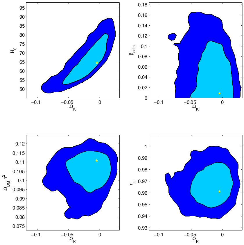
IV.5 Massive neutrinos
Up to now, we have fixed the relative fraction of massive neutrinos to zero. We now consider run cq1 in which we also allow for a non zero fraction of massive neutrinos and marginalize over . In this case the range allowed for the coupling is , slightly bigger than when using massless neutrinos, as expected [41]. We update the results of [41] using both WMAP7 and SPT data. The degeneracy between massive neutrinos and is clearly shown in Fig.13. The best fit value for is

IV.6 Combining WMAP7 and SPT with HST, BAO and Supernovae Ia data
As discussed earlier on in this paper and in [24], the coupling is degenerate with the Hubble parameter. In order to investigate the effect of this degeneracy on the constraints from data, we did another run () in which we combined the data used for (WMAP7 and SPT) to also included baryon acoustic oscillations (BAO) [70], Hubble Space Telescope constraints on (HST) [71] and Supernovae Ia (SNae) data [72] as from COSMOMC (Aug 2011). Likelihood contours for this case are shown in Fig.14. Best fit values and errors are shown in Tab.4, left column. There seems to be an interesting preference for a non zero coupling, though the values are clearly still compatible with zero at 1. This peak comes mostly from a slight tension between the Hubble parameter HST result () and our WMAP7+SPT best fit for ( ). Notice however that even for we are not in an exact CDM since in our model is close, but not exactly equal, to -1. It is interesting then to test whether the forecoming data from Planck can confirm or reject this non zero coupling. This we do in the next section.

IV.7 Combining Planck and SPT mock data
As a further analysis, we forecast the effect that Planck data would have on the coupling parameter, when combined with the power measurement of (run ). Since Planck data are not yet available, we produce a set of mock data [73]. We have therefore implemented FutureCMB [74] in our modified version of COSMOMC and, using as fiducial power spectrum a CDM model , with (black dot-dashed in Fig.15). We have then produced an SPT mock spectrum as follows:
-
we have added to the same fiducial model used to generate Planck mock data, the effect of poisson sources (PS) (blue dotted) using the value for the nuisance parameters with a dependence from the momentum [2];
-
we have added to + PS the effect of clustered sources (CL) (light blue dashed line), using the value for the nuisance parameters with a dependence from the momentum for all . This is not entirely correct as the dependence is slightly different for and but differences are thought to be small [2]; we obtain the . We neglect here the effect of SZ.

| Best fit values | for coupled quintessence | ||
|---|---|---|---|
| Parameter | cq1hst (baseline + +) real data | forecasts | |
| -(Like) |
For this case, we also include BAO, HST and Supernovae Ia data as from Cosmomc (August 2011 version), to break the degeneracy between the coupling and the Hubble parameter. Some representative 2D confidence regions are in Fig. 16. We then find that ; though stronger than WMAP7+SPT, this is still a pessimistic bound, since it includes Planck but still considers SPT data with errors released by [2]; by the time Planck data will be available, better SPT (or ACT) data may have been released. In Table 4 we report the best fit values, together with the left and right errors at and CL around the best fit. The left column refers to run , done with real data (WMAP+SPT+HST+BAO+SNae); the right column shows the forecasted values for Planck+SPT mock data, plus SNae, HST and BAO.

We finally plot in Fig. 17 a comparison between current data and future observations, marginalizing over all parameters except . It is clear that Planck data will reach a precision sufficient to tell whether the peak in is a real detection or just a fluke.

V Conclusions
We have considered the possibility that the evolution of dark matter and dark energy might be connected by a constant coupling, of the type illustrated in [13, 14]. We have used current CMB data from WMAP7 and SPT to constrain the coupling parameter . We find that is constrained to be less than 0.063 (0.11) at () C.L. when SPT data are included, with respect to coming from WMAP7 only. We have done a number of tests to check whether this bound depends on the degeneracy with other parameters (lensing, curvature, massive neutrinos, HST/BAO/SNae data). If the effective number of relativistic degrees of freedom is allowed to vary, no much gain is obtained on , which still needs to be . We have further considered the effect of CMB-lensing, both with a run which includes no lensing and by marginalizing over , a parameter which encodes the rescaling of the lensing power spectrum. is slightly degenerate with which in turn are degenerate with , though no direct degeneracy is seen between and . If the assumption of a flat universe is released, constraints on weaken back almost to the level of constraints given by WMAP only (flat universe), with . Degeneracy with massive neutrinos widens the coupling constraints to be when we marginalize over the fraction of massive neutrino species . We conclude that the bound on from current data is already strong enough to be quite stable with respect to a better knowledge of other parameters and to all cases considered.
When WMAP+SPT are considered (run ), the best fit value for , though still fully compatible with zero, has a best fit of . It is interesting to see that when we allow for an effective number of relativistic degrees of freedom, marginalizing over the coupling from WMAP7+SPT data increases to a best fit value of . A larger value of favors larger couplings between dark matter and dark energy and values of the spectral index closer to . Including SPT data does not improve significantly constraints on the coupling . Inclusion of additional priors from HST, BAO and SNae moves the best fit to , again still compatible with zero at 1. We forecast that the inclusion of Planck data will be able to pin down the coupling to about and therefore detect whether the small non-zero coupling present in current data is washed away with more data.
Acknowledgements.
V.P. is supported by the Marie Curie IEF, Project DEMO - Dark Energy Models and Observations. Support was given to V.P. and C.B. by the Italian Space Agency through the ASI contracts Euclid-IC (I/031/10/0). V.P. thanks Joanna Dunkley for useful discussion and advices. We thank Christof Wetterich for helpful comments. C.B. also acknowledges support from the PD51 INFN initiative. L.A. acknowledges support from DFG - Deutsche Forschungsgemeinschaft through the project TRR33 "The Dark Universe".References
- [1] E. Komatsu, K. M. Smith, J. Dunkley, C. L. Bennett, B. Gold, G. Hinshaw, N. Jarosik, D. Larson, M. R. Nolta, L. Page, et al., The Astrophysical Journal Supplement Series 192, 57 (2010), eprint 1001.4538v3 [astro-ph.CO].
- [2] R. Keisler, C. Reichardt, K. Aird, B. Benson, L. Bleem, et al., Astrophys.J. 743, 28 (2011), eprint 1105.3182.
- [3] S. Das, B. D. Sherwin, P. Aguirre, J. W. Appel, J. Bond, et al., Phys.Rev.Lett. 107, 021301 (2011), eprint 1103.2124.
- [4] A. Lewis and A. Challinor, Physics Reports 429, 1 (2006), eprint arXiv:astro-ph/0601594.
- [5] L. Verde and D. N. Spergel, Phys. Rev. D 65, 043007 (2002), URL http://link.aps.org/doi/10.1103/PhysRevD.65.043007.
- [6] F. Giovi, C. Baccigalupi, and F. Perrotta, ArXiv Astrophysics e-prints (2003), eprint arXiv:astro-ph/0309422.
- [7] V. Acquaviva, C. Baccigalupi, and F. Perrotta, Phys. Rev. D 70, 023515 (2004), eprint arXiv:astro-ph/0403654.
- [8] V. Acquaviva and C. Baccigalupi, Phys. Rev. D 74, 103510 (2006), eprint arXiv:astro-ph/0507644.
- [9] W. Hu, D. Huterer, and K. M. Smith, Astrophys. J. Lett. 650, L13 (2006), eprint arXiv:astro-ph/0607316.
- [10] B. D. Sherwin, J. Dunkley, S. Das, J. W. Appel, J. Bond, et al., Phys.Rev.Lett. 107, 021302 (2011), eprint 1105.0419.
- [11] C. Wetterich, Nucl. Phys. B302, 668 (1988).
- [12] B. Ratra and P. J. E. Peebles, Phys. Rev. D37, 3406 (1988).
- [13] L. Amendola, Phys. Rev. D62, 043511 (2000), eprint astro-ph/9908023.
- [14] V. Pettorino and C. Baccigalupi, Phys. Rev. D77, 103003 (2008a), eprint 0802.1086.
- [15] S. Matarrese, C. Baccigalupi, and F. Perrotta, Phys. Rev. D70, 061301 (2004), eprint astro-ph/0403480.
- [16] F. Perrotta and C. Baccigalupi, Phys. Rev. D65, 123505 (2002), eprint astro-ph/0201335.
- [17] E. Calabrese, R. de Putter, D. Huterer, E. V. Linder, and A. Melchiorri, Phys. Rev. D 83, 023011 (2011), eprint 1010.5612.
- [18] C. L. Reichardt, R. de Putter, O. Zahn, and Z. Hou (2011), eprint 1110.5328.
- [19] J. Khoury and A. Weltman, Phys. Rev. D 69, 044026 (2004), eprint arXiv:astro-ph/0309411.
- [20] L. Hui, A. Nicolis, and C. Stubbs, Phys. Rev. D80, 104002 (2009), eprint 0905.2966.
- [21] A. Upadhye, W. Hu, and J. Khoury, ArXiv e-prints (2012), eprint 1204.3906.
- [22] A.-C. Davis, E. A. Lim, J. Sakstein, and D. J. Shaw, ArXiv e-prints (2011), eprint 1102.5278.
- [23] K. Hinterbichler, J. Khoury, A. Levy, and A. Matas, Phys. Rev. D 84, 103521 (2011), eprint 1107.2112.
- [24] L. Amendola, V. Pettorino, C. Quercellini, and A. Vollmer, Phys. Rev. D 85, 103008 (2012), eprint 1111.1404.
- [25] H. Kodama and M. Sasaki, Prog. Theor. Phys. Suppl. 78, 1 (1984).
- [26] L. Amendola, Phys. Rev. D69, 103524 (2004a), eprint astro-ph/0311175.
- [27] L. Amendola, C. Quercellini, D. Tocchini-Valentini, and A. Pasqui, Astrophys. J. Lett. 583, L53 (2003), eprint astro-ph/0205097.
- [28] L. Amendola and C. Quercellini, Phys. Rev. D 68, 023514 (2003), eprint astro-ph/0303228.
- [29] C. Wetterich, Astron. Astrophys. 301, 321 (1995), eprint hep-th/9408025.
- [30] L. Amendola, Physical Review D 62, 43511 (1999), eprint 9908023.
- [31] G. Mangano, G. Miele, and V. Pettorino, Mod. Phys. Lett. A18, 831 (2003), eprint astro-ph/0212518.
- [32] L. Amendola, Physical Review D 69, 103524 (2004b), eprint 0311175v2.
- [33] T. Koivisto, Phys. Rev. D72, 043516 (2005), eprint astro-ph/0504571.
- [34] Z.-K. Guo, N. Ohta, and S. Tsujikawa, Phys. Rev. D76, 023508 (2007), eprint astro-ph/0702015.
- [35] V. Pettorino and C. Baccigalupi, Phys. Rev. D77, 103003 (2008b), eprint 0802.1086.
- [36] C. Quercellini, M. Bruni, A. Balbi, and D. Pietrobon, Phys. Rev. D 78, 063527 (2008), eprint 0803.1976.
- [37] M. Quartin, M. O. Calvao, S. E. Joras, R. R. R. Reis, and I. Waga, JCAP 0805, 007 (2008), eprint 0802.0546.
- [38] J. Valiviita, R. Maartens, and E. Majerotto, Mon.Not.Roy.Astron.Soc. 402, 2355 (2010), eprint 0907.4987.
- [39] M. Baldi, MNRAS 411, 1077 (2011), eprint 1005.2188.
- [40] R. Bean, E. E. Flanagan, I. Laszlo, and M. Trodden, Phys. Rev. D78, 123514 (2008), eprint 0808.1105.
- [41] G. La Vacca, J. R. Kristiansen, L. P. L. Colombo, R. Mainini, and S. A. Bonometto, JCAP 0904, 007 (2009), eprint 0902.2711.
- [42] J. R. Kristiansen, G. La Vacca, L. P. L. Colombo, R. Mainini, and S. A. Bonometto, New Astron. 15, 609 (2010), eprint 0902.2737.
- [43] N. Wintergerst and V. Pettorino, Phys.Rev. D82, 103516 (2010), eprint 1005.1278.
- [44] R. Mainini and S. Bonometto, Phys. Rev. D74, 043504 (2006), eprint astro-ph/0605621.
- [45] F. Saracco, M. Pietroni, N. Tetradis, V. Pettorino, and G. Robbers, Phys.Rev. D82, 023528 (2010), eprint 0911.5396.
- [46] M. Baldi and V. Pettorino, Mon.Not.Roy.Astron.Soc. 412, L1 (2011), eprint 1006.3761.
- [47] M. Baldi, V. Pettorino, G. Robbers, and V. Springel, Mon. Not. Roy. Astron. Soc. 403, 1684 (2010).
- [48] R. Mainini and D. F. Mota (2010), eprint 1011.0083.
- [49] F. De Bernardis, M. Martinelli, A. Melchiorri, O. Mena, and A. Cooray (2011), eprint 1104.0652.
- [50] J.-Q. Xia, Phys.Rev. D80, 103514 (2009), eprint 0911.4820.
- [51] M. Martinelli, L. L. Honorez, A. Melchiorri, and O. Mena, Phys. Rev. D 81, 103534 (2010), eprint 1004.2410.
- [52] D. Larson, J. Dunkley, G. Hinshaw, E. Komatsu, M. Nolta, et al., Astrophys.J.Suppl. 192, 16 (2011), eprint 1001.4635.
- [53] R. Hlozek, J. Dunkley, G. Addison, J. W. Appel, J. Bond, et al. (2011), eprint 1105.4887.
- [54] A. Lewis, A. Challinor, and A. Lasenby, Astrophys.J. 538, 473 (2000), eprint astro-ph/9911177.
- [55] A. Lewis and S. Bridle, Phys. Rev. D 66, 103511 (2002), eprint arXiv:astro-ph/0205436.
- [56] M. Bartelmann and P. Schneider, Phys. Rept. 340, 291 (2001), eprint astro-ph/9912508.
- [57] C. Carbone, C. Baccigalupi, M. Bartelmann, S. Matarrese, and V. Springel, MNRAS 396, 668 (2009), eprint 0810.4145.
- [58] R. Teyssier, S. Pires, S. Prunet, D. Aubert, C. Pichon, A. Amara, K. Benabed, S. Colombi, A. Refregier, and J.-L. Starck, Astronomy and Astrophysics 497, 335 (2009), eprint 0807.3651.
- [59] D. A. Dicus, E. W. Kolb, A. M. Gleeson, E. C. G. Sudarshan, V. L. Teplitz, and M. S. Turner, Phys. Rev. D 26, 2694 (1982), URL http://link.aps.org/doi/10.1103/PhysRevD.26.2694.
- [60] R. E. Lopez, S. Dodelson, A. Heckler, and M. S. Turner, Phys. Rev. Lett. 82, 3952 (1999), URL http://link.aps.org/doi/10.1103/PhysRevLett.82.3952.
- [61] G. Mangano, G. Miele, S. Pastor, T. Pinto, O. Pisanti, and P. D. Serpico, Nuclear Physics B 729, 221 (2005), eprint arXiv:hep-ph/0506164.
- [62] G. Mangano, G. Miele, S. Pastor, O. Pisanti, and S. Sarikas, J. Cosm. Astroparticle Phys. 3, 35 (2011), eprint 1011.0916.
- [63] J. Dunkley, R. Hlozek, J. Sievers, V. Acquaviva, P. A. R. Ade, P. Aguirre, M. Amiri, J. W. Appel, L. F. Barrientos, E. S. Battistelli, et al., Astrophys. J. 739, 52 (2011), eprint 1009.0866.
- [64] W. Hu and M. White, Physical Review Letters 77, 1687 (1996), eprint arXiv:astro-ph/9602020.
- [65] S. Bashinsky and U. Seljak, Phys. Rev. D 69, 083002 (2004), eprint arXiv:astro-ph/0310198.
- [66] Z. Hou, R. Keisler, L. Knox, M. Millea, and C. Reichardt, ArXiv e-prints (2011), eprint 1104.2333.
- [67] C. L. Reichardt, P. A. R. Ade, J. J. Bock, J. R. Bond, J. A. Brevik, C. R. Contaldi, M. D. Daub, J. T. Dempsey, J. H. Goldstein, W. L. Holzapfel, et al., Astrophys. J. 694, 1200 (2009), eprint 0801.1491.
- [68] E. Calabrese, A. Slosar, A. Melchiorri, G. F. Smoot, and O. Zahn, Phys. Rev. D 77, 123531 (2008), eprint 0803.2309.
- [69] S. Das, T. A. Marriage, P. A. R. Ade, P. Aguirre, M. Amiri, J. W. Appel, L. F. Barrientos, E. S. Battistelli, J. R. Bond, B. Brown, et al., Astrophys. J. 729, 62 (2011), eprint 1009.0847.
- [70] W. J. Percival, B. A. Reid, D. J. Eisenstein, N. A. Bahcall, T. Budavari, J. A. Frieman, M. Fukugita, J. E. Gunn, Ž. Ivezić, G. R. Knapp, et al., MNRAS 401, 2148 (2010), eprint 0907.1660.
- [71] A. G. Riess, L. Macri, S. Casertano, H. Lampeitl, H. C. Ferguson, A. V. Filippenko, S. W. Jha, W. Li, and R. Chornock, Astrophys. J. 730, 119 (2011), eprint 1103.2976.
- [72] R. Amanullah, C. Lidman, D. Rubin, G. Aldering, P. Astier, K. Barbary, M. S. Burns, A. Conley, K. S. Dawson, S. E. Deustua, et al., Astrophys. J. 716, 712 (2010), eprint 1004.1711.
- [73] Planck Collaboration, P. A. R. Ade, N. Aghanim, M. Arnaud, M. Ashdown, J. Aumont, C. Baccigalupi, M. Baker, A. Balbi, A. J. Banday, et al., Astronomy and Astrophysics 536, A1 (2011), eprint 1101.2022.
- [74] L. Perotto, J. Lesgourgues, S. Hannestad, H. Tu, and Y. Y Y Wong, J. Cosm. Astroparticle Phys. 10, 13 (2006), eprint arXiv:astro-ph/0606227.