In the gauge field basis in which the kinetic terms in $\mathscr{L}_{YM}$ are diagonal [33], the covariant derivative reads:

This generic model describes a continuous set of minimal $U(1)$ extensions of the SM, that can be labelled by the charge assignments of the particles [33]. As any other parameter in the Lagrangian, $g_{2}$ and $g_{BL}$ are running parameters, therefore their values have to be set at some scale. Special sets of popular $Z^{\prime}$ models (see, e.g. [29, 55]) can be recovered by imposing relations between $g_{2}$ and $g_{BL}$ at the EW scale. However such relations can be changed through the renormalization group running of the coupling constants [56, 28, 31]. The details of the renormalization group equations (RGEs) are presented in the appendix, as they are not central in the argument of the present paper.

For the following study, it is important to focus on measurable observables, one of which being the $Z^{\prime}$ total width. In the approximation of massless fermions and neutrinos, with $N_{\ell}$ generations of leptinos, of which just the $CP$-odd leptinos ($S_{2}$, the DM candidate) are massive, with in first approximation degenerate masses $M_{S_{2}}$, the total width reads

Since the $S_{2}$ particle is only right-handed, its hypercharge is zero (see table 2), so that its coupling to the $Z^{\prime}$ boson does not depend on $g_{2}$. Moreover, in the evaluation of the DM relic abundance with $S_{2}$ as the DM candidate, we will see that a resonant annihilation with the $Z^{\prime}$ boson is required. In these conditions, $2M_{S_{2}}\sim M_{Z^{\prime}}$ and BR($Z^{\prime}\to S_{2}S_{2}$) $\to 0$. Being around the resonance, the only parameter that can influence the $S_{2}S_{2}\to Z^{\prime}$ partial amplitude, and thus the relic density, is therefore the $Z^{\prime}$ boson width. The smaller the total width, the higher the relative partial amplitude. Hence, the minimum relic density, when one keeps $M_{Z^{\prime}}$ fixed, can be obtained by minimizing the $Z^{\prime}$ width of eq. (3) with respect to $g_{2}$. By direct computation, we obtain that the total $Z^{\prime}$ decay width is minimized for

When $N_{\ell}=1$ (the case discussed here), $g_{2}^{min}=-10/13\,g_{BL}$. Other important cases are for $N_{\ell}=3$ (discussed in section IV in connection with leptogenesis), for which we obtain $g_{2}^{min}=-26/37\,g_{BL}$, and $N_{\ell}=0$, where the minimum width is for the SO(10)-inspired $U(1)_{\chi}$ model, $g_{2}^{min}=-4/5\,g_{BL}$.

So far, we have neglected that the $Z^{\prime}$ boson is in general mixed with the SM $Z$ boson. Typical bounds from LEP-I measurements at the $Z$-boson peak require the mixing angle to be less than $\mathcal{O}(10^{-3})$ [57].

Further, from a combination of LEP-I and LEP-II data the ratio mass-over-coupling is bounded to be bigger than several TeV. In Ref. [32] the authors reanalysed the LEP data for a model with the same gauge sector as ours, while a specific bound for $g_{2}=0$ can also be found in Refs. [29, 58].

Before moving on to the results, we present here (see figure 1) the $95\%$ C.L. exclusions at the LHC in the $g_{BL}-g_{2}$ plane, based on the CMS data at $\sqrt{s}=7$ TeV for the combination of $4.7(4.9)$ fb^-1 in the electron(muon) channels [59]. ATLAS has as well published an analysis for $\sim 5$ fb^-1 [60], but their limits are less tight than the CMS ones. Therefore, we will not present them here.

Table 1 collects the maximum allowed $g_{BL}$ coupling per given $Z^{\prime}$ boson mass for the B-L  model ($g_{2}=0$) and for the $g_{2}^{min}$ case of eq. (4), for $N_{\ell}=1$.

In order to give the $Z^{\prime}$ boson a mass through spontaneous symmetry breaking, an extra complex scalar $\chi$ is introduced. The scalar Lagrangian reads

with the scalar potential given by

where $H$ and $\chi$ are the complex scalar Higgs doublet and singlet fields, respectively.

The scalar sector is now made of two real CP-even scalars, a light one $h_{1}$ and a heavy one $h_{2}$, that are mixtures of the Higgs doublet field and the singlet field:

where $v$($v^{\prime}$) is the VEV of the doublet(singlet) field, while the mixing angle $-\frac{\pi}{2}\leq\alpha\leq\frac{\pi}{2}$ can be expressed as:

with $\lambda_{1,2,3}$ being the parameters entering in the quartic pieces of the scalar potential. The presence of extra heavy neutrinos and the $Z^{\prime}$ boson will alter the properties of the Higgs bosons. The scalar mixing angle $\alpha$ is a free parameter of the model, and the light(heavy) Higgs boson couples to the new matter content proportionally to $\sin{\alpha}$($\cos{\alpha}$), i.e. with the complimentary angle with respect to the interactions with the SM particles.

The B-L -breaking vev $v^{\prime}$ can be expressed in terms of the $Z^{\prime}$ mass and the gauge couplings as follows:

Here we have chosen the B-L  charge of the complex singlet scalar to be $Y^{B\textrm{-}L}_{\chi}=\frac{2}{3}$, as determined by gauge invariance of the Yukawa sector (see the following section).

The LEP bounds on $M_{Z^{\prime}}/g_{BL}$ can provide an absolute lower bound on the VEV $v^{\prime}$ through eq. (9). For the benchmark scenarios of interest here, the bounds are:

We describe here the inverse seesaw mechanism and its implementation in our model. In contrast with the existing literature, we employ renormalizable operators only. The inverse seesaw mechanism can be implemented by means of $N_{\ell}$ extra pairs of RH fields ($S_{1}$ and $S_{2}$) beside the usual $3$ RH neutrinos ($\nu_{R}$), the latter required by the anomaly cancellation. Therefore, the Yukawa Lagrangian for the neutrino sector reads

where $S^{j}_{2}$ are the only odd fields under a $Z_{2}$ symmetry that is introduced to avoid unwanted $S_{1}$–$S_{2}$ mixing. The lightest of the $S^{j}_{2}$ particles is our DM candidate. A summation over $i,j$ is implied and an identical number of $S_{1}$ and $S_{2}$ fields is required by anomaly cancellation. As a concrete model for the DM study, we focus on $N_{\ell}=1$ case. By convention, we choose to implement the inverse seesaw mechanism in the third generation of leptons only. In the following, the formulas will refer to the latter and we drop the “$i$” index, unless otherwise specified. In section III.4 we will show that the DM results do not depend substantially on $N_{\ell}$.

The gauge invariance of the Yukawa Lagrangian is achieved by solving $Y^{B\textrm{-}L}_{S_{1}}+Y^{B\textrm{-}L}_{\chi}=-Y^{B\textrm{-}L}_{\nu_{R}}$ and $2Y^{B\textrm{-}L}_{S_{1}}=\pm Y^{B\textrm{-}L}_{\chi}$, with $Y^{B\textrm{-}L}$ the B-L  charge of the fields. The following two sets of solutions exist, considering that $Y^{B\textrm{-}L}_{\nu_{R}}=1$ is fixed by anomaly cancellations:

• i)

  $Y^{B\textrm{-}L}_{S_{1}}=-1$ and $Y^{B\textrm{-}L}_{\chi}=2$, that is a replica of the type-I B-L  model [38]. In this case, Majorana masses for all the neutrinos would be allowed, as well as a $\overline{\ell_{L}}\widetilde{H}S_{1}$ term. The presence of these terms do not allow for light neutrinos without an extreme fine-tuning of parameters;

• ii)

  $Y^{B\textrm{-}L}_{S_{1}}=1/3$ and $Y^{B\textrm{-}L}_{\chi}=2/3$. This is the new solution proposed here, that forbids all the unwanted terms appearing in (i). Because the B-L  charge is one third of that of the normal leptons and because they do not carry a colour charge, the $S_{1,2}$ fields will be called “leptinos” throughout the rest of this paper.

Table 2 summarises the particle content and the charge assignments.

After spontaneous symmetry breaking, the two Higgs fields acquire vacuum expectation values (called $v$ and $v^{\prime}$, respectively). As a consequence, the first 3 terms of eq (12) lead to the following mass matrix for the interacting neutrinos, in the $(\nu^{c}_{l},\nu_{R},S_{1})$ basis:

where

Eq. (13) is generally referred to as the matrix of the inverse seesaw mechanism. Notice that within the model all the terms appearing in the eq. (13) are proper Yukawa masses. In contrast, in the traditional literature, ${\mathscr{M}^{I}}_{3,3}$ is an effective mass term parametrizing the lepton number violation required for the neutrinos to become massive. In our model, $L$ is spontaneously broken via B-L. When $N_{\ell}=3$ generations of leptinos are considered, $y^{\nu}$ and $y^{s1}$ are in general $3\times 3$ complex matrices, and it is not restrictive to consider $y^{N}$ as a $3\times 3$ real and diagonal matrix.

After diagonalization of eq. (13), the neutrino mass eigenstates are called $\nu_{l}$, $\nu_{h}$ and $\nu_{h^{\prime}}$, with $3\times 3$ mass matrices

However, it is beyond the scope of this paper to consider the most general case in detail. We limit ourselves to the model with only one generation of leptinos, which is largely sufficient for the dark matter question. In this case, one can without loss of generality choose a basis in which both the 3–component vector $y^{N}$ and the single parameter $y^{s1}$ are real. The above formulas simplify, since the seesaw mechanism acts only on the third generation, so that $\mathscr{M}^{I}$ is a $3\times 3$ matrix and eq. (15) gives the masses of the 3 neutrino eigenstates, where $\nu_{h}$ and $\nu_{h^{\prime}}$ combine in a quasi-Dirac fermion. Regarding the first and second generations, the LH and RH neutrinos obtain the usual Dirac mass term, for which $\mathcal{O}(10^{-12})$ Yukawa parameters are required to fit the light neutrino masses.

We present the analytical solution for the inverse seesaw case for $N_{\ell}=1$ which is sufficient to describe the main features of the mechanism also when $N_{\ell}>1$. The mass matrix of eq. (13) is diagonalized by a $3\times 3$ unitary matrix. Such a matrix can be parametrized by $3$ angles and some phases. The latter will be neglected here. Formally, the following generic parametrization can be employed:

where $S_{ij}(C_{ij})=\sin{\alpha_{ij}}(\cos{\alpha_{ij}})$. In good approximation, the angle defining the mixing between $\nu_{R}$ and $S_{1}$ is found to be very close to maximal, i.e., $\alpha_{23}\sim\pi/4$, while the angle parametrizing the mixing between $\nu_{L}$ and $S_{1}$ is very small: $S_{13}\sim M_{D}M_{S_{1}}/M_{N}^{2}\ll 1$. The unitary matrix of eq. (17) can then be simplified to

where $\displaystyle S_{12}\sim\frac{M_{D}}{M_{N}}=\frac{y_{D}v}{y_{N}v^{\prime}}$ controls the mixing between $\nu_{L}$ and $\nu_{R}$. Altogether:

Neglecting intergenerational mixing, eq. (15) can be rewritten as

To obtain light neutrino masses compatible with experiments (i.e., $M_{\nu_{l}}<1$ eV), considering $v^{\prime}=10$ TeV, eq. (20) simplifies to

A possible solution, which allows for the heavy neutrinos in the $\mathcal{O}(100)$ GeV range (suitable for the LHC), requires $y_{N}\sim\mathcal{O}(10^{-2})$. Then, $y_{D}\sim\mathcal{O}(10^{-5})$ implies $y_{s1}<\mathcal{O}(10^{-3})$.

A fundamental difference with the model of Ref. [54] exists in the non-interacting neutrino sector, the $S_{2}$ fields (here we consider only one of them). In eq. (12) it is clear that the $S_{2}$ field acquires a mass after the $U(1)_{B-L}$ symmetry breaking when $\chi$ gets a vev (called $v^{\prime}$):

Therefore, its mass is expected to be of $\mathcal{O}(1)$ TeV, if also $v^{\prime}$ is at TeV scale. The $Z_{2}$ symmetry protects this particle from decaying, making it a suitable dark matter candidate.

We have now all the elements to assess how our model compares to the literature. The most important aspect is that an appropriate neutrino sector is derived combining the extension of the SM gauge group and the inverse seesaw mechanism for the first time in a fully renormalisable way. No new mass scale is required, just the one set by the spontaneous breaking of the new B-L  symmetry, as opposed to the traditional literature for the inverse seesaw mechanism. When this scale is set at the TeV scale, a rich phenomenology for the LHC appears: new particles (the $Z^{\prime}$-boson, two scalar bosons and several heavy neutrinos) and new signatures (for the heavy neutrino signals, see, e.g., Refs. [61, 38, 62]). Our model also provides a solution for the DM and the baryogenesis problems. In the first case, the same $Z_{2}$ symmetry that protects the zeros in the neutrino mass matrix of eq. (13) also stabilises the lightest $S_{2}$ field, that is our DM candidate. The study of the parameter space in which the latter is a viable candidate (i.e., its relic abundance matches the experimentally observed one) is presented in the following section. The baryogenesis problem is solved via the so-called resonant leptogenesis at the TeV scale when large phases in the Dirac neutrino masses are considered. These produce a large $CP$ asymmetry, explaining therefore the observed baryon-antibaryon asymmetry, see section IV. Notice that this mechanism is naturally resonant in the inverse seesaw case, where no fine tuning is required.

For small DM masses, where the main annihilation channel is via the heavy Higgs boson, the relic density is proportional to the $B\textrm{-}L$-breaking vev, since $\Omega h^{2}\propto\frac{1}{\sigma}\propto\frac{1}{y^{2}_{s2}}\propto v^{\prime 2}$, via eq. (22). According to LEP, the vev is constrained from below as in eqs. (10)–(11) for the models of interest. The left panel of figure 3 shows that for $M_{S_{2}}\simeq M_{H_{2}}/2$ the minimal abundance just matches the observed value.

In the right panel of figure 3 we see that the demand, that the resonant $S_{2}$ annihilation proceeds via the Higgs channel, strongly constrains from above the vev $v^{\prime}$ as a function of the heavy Higgs mass $M_{H_{2}}$, $v^{\prime}\leq 11.7$ TeV. It is interesting to note that this upper bound on $v^{\prime}$ is independent of the scalar mixing angle $\alpha$. At the same time, the heavy Higgs mass is constrained from above depending on the value of $\alpha$. For instance for $\sin{\alpha}=0.1,\,M_{H_{2}}\leq 1.8(3.0)$ TeV for $g_{2}=0(g_{2}^{min})$.

Due to LHC direct searches, the $Z^{\prime}$ boson mass has to be above $2\div 2.5$ TeV, depending on the gauge mixing coupling $g_{2}$. For the $Z^{\prime}$ annihilation mechanism to be effective, as already stated, a resonant condition has to be matched, meaning that the DM candidate has to be rather heavy. However, the resonance decay can still be very effective.

Figure 4 shows in more detail that only around the $Z^{\prime}$ resonance the annihilation is sufficient to match the abundance constraint. For simplicity, we fix here $g_{2}=0$, so that the relic density is inversely proportional to the square of the gauge coupling, i.e., $\Omega h^{2}\propto\frac{1}{(g_{BL})^{2}}$. The lower limit on the vev $v^{\prime}$ translates into an upper limit on the coupling, for a fixed $Z^{\prime}$ mass: in figure 4 the $Z^{\prime}$ mass is $2$ TeV, which gives the upper limit $g_{BL}<0.33$, via eq. (9). Then, the demand $\Omega h^{2}\simeq 0.1$ gives a lower limit for the gauge coupling, $g_{BL}>0.21$.

Although the gauge coupling $g_{BL}$ is expected to give the major contribution to the relic abundance evaluation, the impact of $g_{2}$ might be not negligible either. For fixed $M_{Z^{\prime}}$ and $g_{BL}$ values, we study here the effect of the mixing gauge coupling. We choose two different sets of $M_{Z^{\prime}}$ and $g_{BL}$ such that for $g_{2}=0$ the relic density just satisfies the abundance constraint. Figure 5 then shows that $g_{2}$ can have an impact on the relic abundance, in particular it can lower the latter when assuming small negative values.

A general feature is that $\Omega(g_{2})$ is growing for $|g_{2}|\to 1$, so that there exists a value of $g_{2}$ that minimizes $\Omega(g_{2})$. This value of $g_{2}$ corresponds to the $g_{2}^{min}$ of eq. (4), that also minimizes the $Z^{\prime}$ width. Fixing $g_{2}$ to $g_{2}^{min}(g_{BL})$ returns a minimum value for $g_{BL}$ such that the abundance constraint can be matched, which is roughly $5\%$ lower than the lower limit on $g_{BL}$ in the case $g_{2}=0$. We can now study the relic density as a function of the $Z^{\prime}$ boson mass. This is done in figure 6, that shows the range of allowed values for $g_{BL}$ as a function of $M_{Z^{\prime}}$. The curves, for both $g_{2}=0$ and $g_{2}=g_{2}^{min}(g_{BL})$, limit the existence of a DM candidate mass with suitable relic density above the curves themselves.

As a result, the $Z^{\prime}$ mass is constrained to $M_{Z^{\prime}}\leq 3.5(5.0)$ TeV for the $g_{2}=0$ and the $g_{2}=g_{2}^{min}(g_{BL})$ case, respectively, which also imposes an upper bound on the gauge couplings when combined with the exclusion limits from LEP. Notice that this value for the $Z^{\prime}$ mass is within the LHC ultimate reach [41]. Since we must be on a resonant regime, the upper bound on the $Z^{\prime}$ mass translates on a upper bound for the $S_{2}$ mass, $M_{S_{2}}\leq 2.5$ TeV.

The spin independent leptino-nucleon interaction is mediated by the light Higgs boson and is therefore sensitive to the value of $(\sin{\alpha}\cos{\alpha})^{2}$. Figure 7 shows that even for the rather large value of $\sin{\alpha}=0.3$, the leptino-nucleon cross section is several orders of magnitude below the actual exclusion limits from XENON100 [68], at most of roughly $10^{-44}$ $\text{cm}^{2}$ for a DM candidate mass of around $50$ GeV. Since we know that $\sin{\alpha}$ has to be small, also future direct detection experiments will not be able to restrict or to detect the leptino. We checked that the exchange of $Z^{\prime}$ bosons consistent with LEP exclusion limits gives rise to smaller cross sections than Higgs exchange, hence we did not further consider this process. Even easier to evade are the constraints from spin-dependent leptino-nucleon interaction experiments. Here the only mediator that can play a role is the $Z^{\prime}$ boson, too heavy for these cross sections to be of any interest.

As we will discuss in the next section, a successful leptogenesis needs $N_{\ell}\geq 2$ to provide the required large $CP$–violating phases. Here we want to comment on the impact of extra leptino generations in the DM analysis carried out so far. The extra neutrinos affect the $Z^{\prime}$ width only, see eq. (3), and will be discussed later. First we focus on the leptinos. If the $S_{2}^{i}$ fields possess a large mass hierarchy, the heavier particles decouple earlier and decay rapidly to the still thermalized lighter particles. If they are exactly mass degenerate, however, we get $\Omega_{N_{\ell}}=N_{\ell}\cdot\Omega_{1}$. Thus to have resonant annihilation the couplings have to be increased by $\sqrt{N_{\ell}}$. Figure 8 shows how this affects the parameter space. For resonant heavy Higgs annihilation the vev $v^{\prime}$ must be reduced by a factor $\sqrt{N_{\ell}}$, so that only the cases $N_{\ell}=1,2$ can still match the relic abundance for Higgs resonant annihilation, while $N_{\ell}=3$ is just touching the LEP exclusion limits (for $g_{2}=g_{2}^{min}$) from below and therefore such resonant mechanism is not sufficient.

The case of resonant $Z^{\prime}$ annihilation works well also for $N_{\ell}=3$. However, the allowed parameter space becomes tighter for higher $N_{\ell}$. These results are valid when all the leptinos are mass degenerate, and represents the worst possible case. All others, i.e. when just 2 are degenerate or with a tight mass hierarchy, will be somewhere between the case of $1$ generation and the case of $3$ generations exactly degenerate in mass. Notice that when the leptinos possess a tight mass hierarchy also co-annihilation processes become important and have to be taken into account. However their inclusion will not change the results.

We turn now to study the effect of having $3$ generations of leptinos, as required for leptogenesis, on the dark matter relic abundance due to the extra heavy neutrinos. The model with $3$ generations of leptinos has $3$ light and $6$ heavy Majorana neutrinos in total. The one with only $1$ generation of leptinos instead accounts for $3$ light neutrinos, $2$ of them being Dirac particles, and $2$ heavy Majorana neutrinos. Although the total number of relativistic degrees of freedom, commonly addressed as $g^{\ast}$, is basically unchanged, the proliferation of neutrinos affects the $Z^{\prime}$ width, and this could impinge on the evaluation of the relic abundance at the $Z^{\prime}$ resonance. Figure 9 shows the total $Z^{\prime}$ width in the $2$ different cases, $N_{\ell}=1,3$.

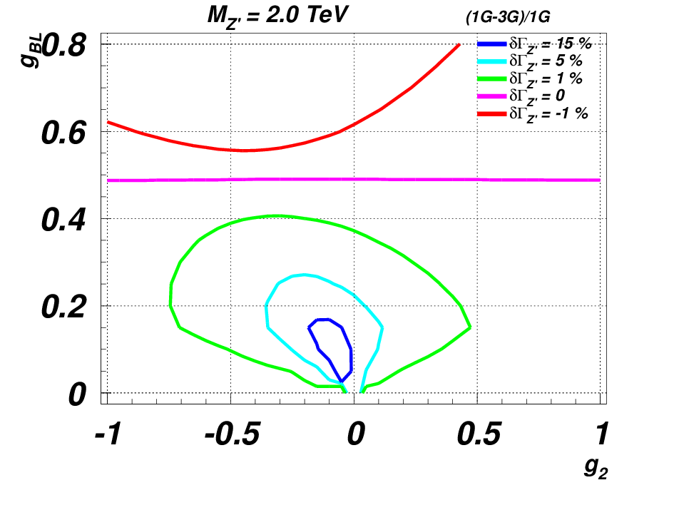
Despite the larger numbers of possible final states into which the $Z^{\prime}$ boson can decay for $N_{\ell}=3$ with respect to $N_{\ell}=1$, the latter case has a larger $Z^{\prime}$ boson partial width into light neutrinos since 2 of them are Dirac particles. Moreover, finite mass and threshold effects for the heavy neutrinos diminish their branching ratios. Altogether, this induces an almost exact compensation between the larger number of heavy neutrinos for $N_{\ell}=3$ and the larger partial width due to the $2$ Dirac light neutrinos for $N_{\ell}=1$. The relative variation of the total $Z^{\prime}$ width is below $1\%$ in most of the parameter space, getting above $5\%$ only in a limited region around small values of the gauge couplings. In these plots, heavy neutrino masses are $m_{h\nu}=637$ GeV for $g_{BL}=0.2$, and scale inversely with the latter. When their mass is above $M_{Z^{\prime}}/2$ (or slightly before due to threshold effects, i.e., here for $g_{BL}<0.15$), the $Z^{\prime}\to NN$ ($N=\nu_{h},\,\nu{{}_{h}^{\prime}}$) channels are all suppressed or simply forbidden and the above mentioned compensation is not taking place. Even though the model with $1$ generation of leptinos has here a bigger $Z^{\prime}$ width due to the larger partial widths into the light Dirac neutrinos, the excess is never above $20\%$ of the total $Z^{\prime}$ width in the case of $3$ generations, and only in a tiny corner of the parameter space, where both gauge couplings are small.

As intimated, the variation of the total $Z^{\prime}$ width is very small, mostly below $1\%$, so that the impact on the DM relic abundance is also negligible. This is because, the relic abundance scales with the square root of the $Z^{\prime}$ width. A $1\%$ variation in the total width determines a $0.5\%$ variation of the relic density.

We can conclude that the DM study for $N_{\ell}=1$ of section III is independent of the particular value of $N_{\ell}$ if the leptinos are not mass degenerate.

As discussed in the introduction, the inverse seesaw mechanism is a suitable mechanism for a large $CP$ asymmetry even at the TeV scale due to the naturally small mass splitting between the heavier neutrino eigenstates, a result that is built in into the model and does not require fine tuning. Hence, it is a favourable model for the so-called resonant leptogenesis. Despite a large loop enhancement due to resonance, large phases are still required in the off-diagonal terms of $y_{D}$ to obtain an $\mathcal{O}(1)$ $CP$ asymmetry. In the $N_{\ell}=1$ model discussed so far, the first 2 generations of light neutrinos require $\mathcal{O}(10^{-12})$ Yukawas, which in turn also means that the $CP$–violating decays of the heavy Majorana neutrino pair are similarly suppressed. Large phases but small masses can be achieved extending the seesaw mechanism to the other generations.

We show here that leptogenesis, compatible with neutrino masses and mixing, is possible in this model. The $CP$ asymmetry is generated by the decays of the heavy neutrinos:

requiring large phases in the off-diagonal elements of the Dirac Yukawa matrix $y_{D}$. In our model, these large phases, compatible with neutrino data, are possible for $N_{l}\geq 2$. The lepton number violating loop factor $f^{\nu}_{ij}$, when quasi-degenerate heavy neutrino pairs are considered, is

In the inverse seesaw case, $M_{j}\sim M_{i}$ and $\Gamma_{j}=\Gamma_{i}\equiv\Gamma$ are naturally recovered, so that $f^{\nu}_{ij}$ can easily be $\mathcal{O}(1)$. Notice that no fine tuning is required.

Once an asymmetry in the lepton sector is produced, electroweak sphaleron processes take place and move the asymmetry to the baryon sector $\displaystyle\eta_{B}=\frac{28}{79}\eta_{B-L}$. Altogether, the final baryon asymmetry can be written as

where the $10^{-2}$ pre-factor accounts for the sphaleron efficiency and for photon dilution after recombination. The $CP$ asymmetry $\varepsilon_{i}$ was defined in eq. (24), while $\kappa_{i}$ is the efficiency factor obtained after solving the relevant Boltzmann equations:

with $\displaystyle\delta_{i}=\frac{\left|M_{i}-M_{j}\right|}{\Gamma}\ll 1$ suppresses considerably the inverse decay (ID) wash-out.

All the quantities are defined in Ref. [53]. Particularly important is the $S_{Z^{\prime}}$ term, the $Z^{\prime}$ scattering processes, which induces a wash-out of the final asymmetry. It has been verified that these $Z^{\prime}$–induced wash-out processes do not have a severe impact on the final baryon asymmetry. This is due to the nature of the inverse seesaw mechanism, that allows for large Yukawa couplings, overcoming the $Z^{\prime}$ processes. A similar conclusion was reached in Ref. [46], in which the authors explicitly showed that $Z^{\prime}$ processes do not spoil the leptogenesis if the Dirac Yukawa couplings are sufficiently large, as in the inverse seesaw case under examination.

In conclusion, following the similar case studied in Ref. [53], the Dirac Yukawa matrix $y_{D}$ contains all information required to study the leptogenesis, entering both in $\varepsilon_{i}$ and in $\Gamma$. It is sufficient that some off-diagonal elements in $y_{D}$ are large and complex for leptogenesis to be possible. For definiteness, we have verified that the choice of the matrix in Ref. [53], that for $N_{l}=3$ is a possibility in our setup, does yield the correct baryon asymmetry in our model. We stress again that a similar choice for $y_{D}$ compatible with a successful leptogenesis is possible also for $N_{l}=2$, even though only one off-diagonal element will be large in this case. This is in fact identical to $N_{l}=3$ in the 1-flavour approximation.

Hence, we have proven that a successful leptogenesis, compatible with the observed pattern of neutrino masses and mixing angles is possible in our model when at least two generations of leptinos are present. However, the complete analysis of the leptogenesis in our model, as for instance the detailed comparison of $N_{l}=2$ and $N_{l}=3$ cases, or the impact of flavour effects outside the simple 1-flavour analysis, is beyond the scope of this paper and is left for future work.

As a last application of our model, we describe the possible implications on $N^{\nu}_{eff}$. This observable counts the relativistic energy content in the universe at the time of the last scattering surface in terms of an effective number of neutrino species. Indications from cosmology result in the observed value of $N^{CMB}_{eff}=4.56\pm 0.75$ when combining WMAP, the Atacama Cosmology Telescope, baryonic acoustic oscillations data and the measurement of the Hubble parameter $H_{0}$ [69]. Notice that the SM LH neutrinos only would yield $N^{\nu}_{eff}\sim 3$. This mismatch is typically interpreted as an indication of the existence of some extra relativistic degrees of freedom that effectively contribute as one unit of $N^{\nu}_{eff}$. In our setup, the only extra degrees of freedom that can be relativistic at the last scattering surface are the RH neutrinos, when they have only Dirac mass terms, i.e., for less than $3$ generations of leptinos, as described in section III.4. On the other hand, as we have seen previously, a successful leptogenesis requires more than one generation of leptinos. If one would like to explain both leptogenesis and $\Delta N^{\nu}_{eff}$ in our model, less than three generations of leptinos should be considered, given that $N_{\ell}=3$ leads to an effective number $N^{\nu}_{eff}\sim 3$ as in the standard model.

An estimate of the impact on $N^{\nu}_{eff}$ is done as follows. First, the decoupling temperature and the contribution to $N^{\nu}_{eff}$ depend on the parameters $m_{Z^{\prime}}$, $g_{BL}$, $g_{2}$, given that only the $Z^{\prime}$ boson can keep the RH neutrinos in thermal equilibrium with electrons, as the RH neutrinos have vanishing hypercharge. Naively, the bigger the $Z^{\prime}$ cross section, the lower the decoupling temperature, which in turns also means that less degrees of freedom are relativistic at decoupling. Overall, this increases the RH neutrino contribution to $N^{\nu}_{eff}$. Close to LEP exclusion limits, we get a minimum decoupling temperature of $~380$ MeV. At this temperature the number of relativistic degrees of freedom is $20$ if the QCD phase transition takes place at $450$ MeV [70]. This yields the highest value for $\Delta N^{\nu}_{eff}$ in our model: $0.18\,(3-N_{\ell})$. For lower QCD phase transition temperatures, the numbers of relativistic degrees of freedom rapidly increases, suppressing the impact on $N^{\nu}_{eff}$ to the percent level or below.

Thus we see that although the model can contribute to $N^{\nu}_{eff}$, its impact is only marginal, especially if one would want to implement a successful leptogenesis. In fact, $N_{\ell}\geq 2$ is required by the latter, while $N_{\ell}\to 0$ maximises $\Delta N^{\nu}_{eff}$.

References

- [1] P. Minkowski, Phys. Lett. B67, 421 (1977)
- [2] P. R. M. Gell-Mann and R. Slansky in Supergravity, edited by P. Van Nieuwenhuizen and D. Z. Freedman (North-Holland, Amsterdam, 1979), p. 341
- [3] T. Yanagida in Proceedings of the Workshop on the Baryon Number of the Universe and Unified Theories, edited by O. Sawada and A. Sugamoto, (KEK, Tsukuba, 1979), p 95
- [4] S.L. Glashow, in Quarks and Leptons, eds. M.Lèvy et al. (Plenum, New York ), p.
- [5] R. N. Mohapatra and G. Senjanovic, Phys. Rev. Lett. 44, 912 (1980)
- [6] R. Mohapatra and J. Valle D34, 1642 (1986)
- [7] R. Mohapatra, Phys.Rev.Lett. 56, 561 (1986)
- [8] M. Fukugita and T. Yanagida, Phys.Lett. B174, 45 (1986)
- [9] M. Plumacher, Z.Phys. C74, 549 (1997)
- [10] W. Buchmuller, P. Di Bari, and M. Plumacher, Annals Phys. 315, 305 (2005)
- [11] S. Davidson, E. Nardi, and Y. Nir, Phys.Rept. 466, 105 (2008)
- [12] L. Canetti and M. Shaposhnikov, JCAP 1009, 001 (2010)
- [13] V. Kuzmin, V. Rubakov, and M. Shaposhnikov, Phys.Lett. B155, 36 (1985)
- [14] S. Khlebnikov and M. Shaposhnikov, Nucl.Phys. B308, 885 (1988)
- [15] Y. Burnier, M. Laine, and M. Shaposhnikov, JCAP 0602, 007 (2006)
- [16] M. Flanz, E. A. Paschos, U. Sarkar, and J. Weiss, Phys.Lett. B389, 693 (1996)
- [17] L. Covi, E. Roulet, and F. Vissani, Phys.Lett. B384, 169 (1996)
- [18] A. Pilaftsis, Phys.Rev. D56, 5431 (1997)
- [19] R. Barbieri, P. Creminelli, A. Strumia, and N. Tetradis, Nucl.Phys. B575, 61 (2000)
- [20] A. Pilaftsis and T. E. Underwood, Nucl.Phys. B692, 303 (2004)
- [21] A. Pilaftsis and T. E. Underwood, Phys.Rev. D72, 113001 (2005)
- [22] A. Abada, S. Davidson, F.-X. Josse-Michaux, M. Losada, and A. Riotto, JCAP 0604, 004 (2006)
- [23] S. Blanchet and P. Di Bari, JCAP 0703, 018 (2007)
- [24] A. Abada, S. Davidson, A. Ibarra, F.-X. Josse-Michaux, M. Losada, et al., JHEP 0609, 010 (2006)
- [25] E. Nardi, Y. Nir, E. Roulet, and J. Racker, JHEP 0601, 164 (2006)
- [26] D. Aristizabal Sierra, M. Losada, and E. Nardi, JCAP 0912, 015 (2009)
- [27] ICHEP-Conference, Melbourne 2012
- [28] F. del Aguila, M. Masip, and M. Perez-Victoria, Nucl. Phys. B456, 531 (1995)
- [29] M. S. Carena, A. Daleo, B. A. Dobrescu, and T. M. P. Tait, Phys. Rev. D70, 093009 (2004)
- [30] P. H. Chankowski, S. Pokorski, and J. Wagner, Eur. Phys. J. C47, 187 (2006)
- [31] A. Ferroglia, A. Lorca, and J. van der Bij, Annalen Phys. 16, 563 (2007)
- [32] E. Salvioni, G. Villadoro, and F. Zwirner, JHEP 11, 068 (2009)
- [33] L. Basso, S. Moretti, and G. M. Pruna, JHEP 1108, 122 (2011)
- [34] E. E. Jenkins, Phys. Lett. B192, 219 (1987)
- [35] W. Buchmuller, C. Greub, and P. Minkowski, Phys. Lett. B267, 395 (1991)
- [36] S. Khalil, J. Phys. G35, 055001 (2008)
- [37] K. Huitu, S. Khalil, H. Okada, and S. K. Rai, Phys. Rev. Lett. 101, 181802 (2008)
- [38] L. Basso, A. Belyaev, S. Moretti, and C. H. Shepherd-Themistocleous, Phys. Rev. D80, 055030 (2009)
- [39] P. Fileviez Perez, T. Han, and T. Li, Phys. Rev. D80, 073015 (2009)
- [40] S. Iso, N. Okada, and Y. Orikasa, Phys. Lett. B676, 81 (2009)
- [41] L. Basso, A. Belyaev, S. Moretti, G. M. Pruna, and C. H. Shepherd-Themistocleous, Eur.Phys.J. C71, 1613 (2011)
- [42] L. Basso, S. Moretti, and G. M. Pruna, Phys.Rev. D83, 055014 (2011)
- [43] N. Sahu and U. A. Yajnik, Phys.Rev. D71, 023507 (2005)
- [44] M. Abbas and S. Khalil, JHEP 04, 056 (2008)
- [45] S. Blanchet, Z. Chacko, S. S. Granor, and R. N. Mohapatra, Phys.Rev. D82, 076008 (2010)
- [46] S. Iso, N. Okada, and Y. Orikasa, Phys.Rev. D83, 093011 (2011)
- [47] N. Okada and O. Seto, Phys.Rev. D82, 023507 (2010)
- [48] R. Hernandez-Pinto and A. Perez-Lorenzana(2011), arXiv:1104.2384 [hep-ph]
- [49] S. Kanemura, T. Nabeshima, and H. Sugiyama, Phys.Rev. D85, 033004 (2012)
- [50] N. Okada and Y. Orikasa, Phys.Rev. D85, 115006 (2012)
- [51] J. Garayoa, M. Gonzalez-Garcia, and N. Rius, JHEP 0702, 021 (2007)
- [52] S. Blanchet, T. Hambye, and F.-X. Josse-Michaux, JHEP 1004, 023 (2010)
- [53] S. Blanchet, P. Dev, and R. Mohapatra, Phys.Rev. D82, 115025 (2010)
- [54] S. Khalil, Phys. Rev. D82, 077702 (2010)
- [55] T. Appelquist, B. A. Dobrescu, and A. R. Hopper, Phys. Rev. D68, 035012 (2003)
- [56] F. del Aguila, G. D. Coughlan, and M. Quiros, Nucl. Phys. B307, 633 (1988)
- [57] J. Erler, P. Langacker, S. Munir, and E. R. Pena, JHEP 08, 017 (2009)
- [58] G. Cacciapaglia, C. Csaki, G. Marandella, and A. Strumia, Phys. Rev. D74, 033011 (2006)
- [59] Https://twiki.cern.ch/twiki/bin/view/CMSPublic/PhysicsResultsEXO11019Winter2012
- [60] ATLAS-CONF-2012-007
- [61] F. del Aguila and J. Aguilar-Saavedra, Nucl.Phys. B813, 22 (2009)
- [62] M. Hirsch, T. Kernreiter, J. Romao, and A. Villanova del Moral, JHEP 1001, 103 (2010)
- [63] G. Belanger, F. Boudjema, A. Pukhov, and A. Semenov, Comput.Phys.Commun. 149, 103 (2002)
- [64] G. Belanger, F. Boudjema, A. Pukhov, and A. Semenov, Comput.Phys.Commun. 174, 577 (2006)
- [65] A. V. Semenov(1996), arXiv:hep-ph/9608488
- [66] A. Pukhov(2004), arXiv:hep-ph/0412191
- [67] CMS and ATLAS talks on July 2012, http://indico.cern.ch/conferenceDisplay.py?confId=197461
- [68] E. Aprile et al. (XENON100), Phys. Rev. Lett. 107, 131302 (2011)
- [69] J. Dunkley, R. Hlozek, J. Sievers, V. Acquaviva, P. Ade, et al., Astrophys.J. 739, 52 (2011)
- [70] J. Beringer et al. (Particle Data Group), Phys. Rev. D86, (2012).
- [71] L. Basso, S. Moretti, and G. M. Pruna, Phys. Rev. D82, 055018 (2010)