Expectation-maximization Gaussian-mixture Approximate Message Passing
Abstract
When recovering a sparse signal from noisy compressive linear measurements, the distribution of the signal’s non-zero coefficients can have a profound effect on recovery mean-squared error (MSE). If this distribution was apriori known, then one could use computationally efficient approximate message passing (AMP) techniques for nearly minimum MSE (MMSE) recovery. In practice, though, the distribution is unknown, motivating the use of robust algorithms like LASSO—which is nearly minimax optimal—at the cost of significantly larger MSE for non-least-favorable distributions. As an alternative, we propose an empirical-Bayesian technique that simultaneously learns the signal distribution while MMSE-recovering the signal—according to the learned distribution—using AMP. In particular, we model the non-zero distribution as a Gaussian mixture, and learn its parameters through expectation maximization, using AMP to implement the expectation step. Numerical experiments on a wide range of signal classes confirm the state-of-the-art performance of our approach, in both reconstruction error and runtime, in the high-dimensional regime, for most (but not all) sensing operators.
I Introduction
We consider estimating a -sparse (or compressible) signal from linear measurements , where is known and is additive white Gaussian noise (AWGN). For this problem, accurate (relative to the noise variance) signal recovery is known to be possible with polynomial-complexity algorithms when is sufficiently sparse and when satisfies certain restricted isometry properties [4], or when is large with i.i.d zero-mean sub-Gaussian entries [5] as discussed below.
LASSO [6] (or, equivalently, Basis Pursuit Denoising [7]), is a well-known approach to the sparse-signal recovery problem that solves the convex problem
| (1) |
with a tuning parameter that trades between the sparsity and measurement-fidelity of the solution. When is constructed from i.i.d zero-mean sub-Gaussian entries, the performance of LASSO can be sharply characterized in the large system limit (i.e., as with fixed undersampling ratio and sparsity ratio ) using the so-called phase transition curve (PTC) [8, 5]. When the observations are noiseless, the PTC bisects the -versus- plane into the region where LASSO reconstructs the signal perfectly (with high probability) and the region where it does not. (See Figs. 3–5.) When the observations are noisy, the same PTC bisects the plane into the regions where LASSO’s noise sensitivity (i.e., the ratio of estimation-error power to measurement-noise power under the worst-case signal distribution) is either finite or infinite [9]. An important fact about LASSO’s noiseless PTC is that it is invariant to the distribution of the nonzero signal coefficients. In other words, if the vector is drawn i.i.d from the pdf
| (2) |
where is the Dirac delta, is the active-coefficient pdf (with zero probability mass at ), and , then the LASSO PTC is invariant to . While this implies that LASSO is robust to “difficult” instances of , it also implies that LASSO cannot benefit from the case that is an “easy” distribution. For example, when the signal is known apriori to be nonnegative, polynomial-complexity algorithms exist with PTCs that are better than LASSO’s [10].
At the other end of the spectrum is minimum mean-squared error (MMSE)-optimal signal recovery under known marginal pdfs of the form (2) and known noise variance. The PTC of MMSE recovery has been recently characterized [11] and shown to be well above that of LASSO. In particular, for any , the PTC on the -versus- plane reduces to the line in both the noiseless and noisy cases. Moreover, efficient algorithms for approximate MMSE-recovery have been proposed, such as the Bayesian version of Donoho, Maleki, and Montanari’s approximate message passing (AMP) algorithm from [12], which performs loopy belief-propagation on the underlying factor graph using central-limit-theorem approximations that become exact in the large-system limit under i.i.d zero-mean sub-Gaussian . In fact, in this regime, AMP obeys [13] a state-evolution whose fixed points, when unique, are optimal. To handle arbitrary noise distributions and a wider class of matrices , Rangan proposed a generalized AMP (GAMP) [14] that forms the starting point of this work. (See Table I.) For more details and background on GAMP, we refer the reader to [14].
In practice, one ideally wants a recovery algorithm that does not need to know and the noise variance a priori, yet offers performance on par with MMSE recovery, which (by definition) requires knowing these prior statistics. Towards this goal, we propose a recovery scheme that aims to learn the prior signal distribution , as well as the variance of the AWGN, while simultaneously recovering the signal vector from the noisy compressed measurements . To do so, we model the active component in (2) using a generic -term Gaussian mixture (GM) and then learn the GM parameters and noise variance using the expectation-maximization (EM) algorithm [15]. As we will see, all of the quantities needed for the EM updates are already computed by the GAMP algorithm, making the overall process very computationally efficient. Moreover, GAMP provides approximately MMSE estimates of that suffice for signal recovery, as well as posterior activity probabilities that suffice for support recovery.
Since, in our approach, the prior pdf parameters are treated as deterministic unknowns, our proposed EM-GM-AMP algorithm can be classified as an “empirical-Bayesian” approach [16]. Compared with previously proposed empirical-Bayesian approaches to compressive sensing (e.g., [17, 18, 19]), ours has a more flexible signal model, and thus is able to better match a wide range of signal pdfs , as we demonstrate through a detailed numerical study. In addition, the complexity scaling of our algorithm is superior to that in [17, 18, 19], implying lower complexity in the high dimensional regime, as we confirm numerically. Supplemental experiments demonstrate that our excellent results hold for a wide range of sensing operators , with some exceptions. Although this paper does not contain any convergence guarantees or a rigorous analysis/justification of the proposed EM-GM-AMP, Kamilov et al. showed (after the submission of this work) in [20] that a generalization of EM-GM-AMP yields asymptotically (i.e., in the large system limit) consistent parameter estimates when is i.i.d zero-mean Gaussian, when the parameterized signal and noise distributions match the true signal and noise distributions, and when those distributions satisfy certain identifiability conditions. We refer interested readers to [20] for more details.
Notation: For matrices, we use boldface capital letters like , and we use and to denote the trace and Frobenius norm, respectively. Moreover, we use , , and to denote transpose, conjugate, and conjugate transpose, respectively. For vectors, we use boldface small letters like , and we use to denote the norm, with representing the element of . For a Gaussian random vector with mean and covariance matrix , we denote the pdf by , and for its circular complex Gaussian counterpart, we use . Finally, we use , , , and to denote the expectation operation, the Dirac delta, the real field, and the complex field, respectively.
II Gaussian-Mixture GAMP
We first introduce Gaussian-mixture (GM) GAMP, a key component of our overall approach, where the coefficients in are assumed to be i.i.d with marginal pdf
| (3) |
where is the Dirac delta, is the sparsity rate, and, for the GM component, , , and are the weight, mean, and variance, respectively. In the sequel, we use and similar definitions for and . By definition, . The noise is assumed to be i.i.d Gaussian, with mean zero and variance , i.e.,
| (4) |
and independent of . Although above and in the sequel we assume real-valued quantities, all expressions in the sequel can be converted to the circular-complex case by replacing with and removing the ’s from (25), (44), and (58). We note that, from the perspective of GM-GAMP, the prior parameters and the number of mixture components, , are treated as fixed and known.
GAMP models the relationship between the observed output and the corresponding noiseless output , where denotes the row of , using the conditional pdf . It then approximates the true marginal posterior by
| (5) |
using quantities and that change with iteration (see Table I), although here we suppress the notation for brevity. Under the AWGN assumption11 1 Because GAMP can handle an arbitrary , the extension of EM-GM-AMP to additive non-Gaussian noise, and even non-additive measurement channels (such as with quantized outputs [21] or logistic regression [14]), is straightforward. Moreover, the parameters of the pdf could be learned using a method similar to that which we propose for learning the AWGN variance , as will be evident from the derivation in Section III-A. Finally, one could even model as a Gaussian mixture and learn the corresponding parameters. (4) we have , and thus the pdf (5) has moments [14]
| (6) | ||||
| (7) |
GAMP then approximates the true marginal posterior by
| (8) |
where again and vary with the GAMP iteration .
Plugging the sparse GM prior (3) into (8) and simplifying, one can obtain22 2 Both (10) and (12) can be derived from (9) via the Gaussian-pdf multiplication rule: . the GM-GAMP approximated posterior
| (9) | |||||
| (10) | |||||
with normalization factor
| (11) | |||
| (12) |
and -dependent quantities
| (13) | ||||
| (14) | ||||
| (15) | ||||
| (16) | ||||
| (17) |
The posterior mean and variance of are given in steps (R9)-(R10) of Table I, and (10) makes it clear that is GM-GAMP’s approximation of the posterior support probability .
In principle, one could specify GAMP for an arbitrary signal prior . However, if the integrals in (R9)–(R10) are not computable in closed form (e.g., when is Student’s-t), then they would need to be computed numerically, thereby drastically increasing the computational complexity of GAMP. In contrast, for GM signal models, we see above that all steps can be computed in closed form. Thus, a practical approach to the use of GAMP with an intractable signal prior is to approximate using an -term GM, after which all GAMP steps can be easily implemented. The same approach could also be used to ease the implementation of intractable output priors .
III EM Learning of the Prior Parameters
We now propose an expectation-maximization (EM) algorithm [15] to learn the prior parameters . The EM algorithm is an iterative technique that increases a lower bound on the likelihood at each iteration, thus guaranteeing that the likelihood converges to a local maximum or at least a saddle point [22]. In our case, the EM algorithm manifests as follows. Writing, for arbitrary pdf ,
| (18) | ||||
| (19) | ||||
| (20) |
where denotes expectation over , denotes the entropy of pdf , and denotes the Kullback-Leibler (KL) divergence between and . The non-negativity of the KL divergence implies that is a lower bound on , and thus the EM algorithm iterates over two steps: E) choosing to maximize the lower bound for fixed , and M) choosing to maximize the lower bound for fixed . For the E step, since , the maximizing pdf would clearly be , i.e., the true posterior under prior parameters . Then, for the M step, since , the maximizing would clearly be .
In our case, because the true posterior is very difficult to calculate, we instead construct our lower-bound using the GAMP approximated posteriors, i.e., we set for defined in (8), resulting in
| (21) |
where “” indicates the use of the GAMP’s posterior approximation. Moreover, since the joint optimization in (21) is difficult to perform, we update one component at a time (while holding the others fixed), which is the well known “incremental” variant on EM from [23]. In the sequel, we use “” to denote the vector with the element removed (and similar for the other parameters).
III-A EM Update of the Gaussian Noise Variance
We first derive the EM update for the noise variance given a previous parameter estimate . For this, we write for a -invariant constant , so that
| (22) | |||||
| (23) | |||||
since . The maximizing value of in (23) is necessarily a value of that zeroes the derivative of the sum, i.e., that satisfies33 3 The continuity of both the integrand and its partial derivative with respect to allow the use of Leibniz’s integral rule to exchange differentiation and integration.
| (24) |
Because , we can obtain
| (25) |
which, when plugged into (24), yields the unique solution
| (26) | ||||
| (27) |
where the use of and follows from (R3)-(R4) in Table I.
III-B EM Updates of the Signal Parameters: BG Case
Suppose that the signal distribution is modeled using an -term GM, i.e., a Bernoulli-Gaussian (BG) pdf. In this case, the marginal signal prior in (3) reduces to
| (28) |
Note that, in the BG case, the mixture weight is, by definition, unity and does not need to be learned.
We now derive the EM update for given previous parameters . Because we can write for a -invariant constant ,
| (29) |
The maximizing value of in (29) is necessarily a value of that zeroes the derivative of the sum, i.e., that satisfies44 4 To justify the exchange of differentiation and integration via Leibniz’s integral rule here, one could employ the Dirac approximation for fixed arbitrarily small , after which the integrand and its derivative w.r.t become continuous. The same comment applies in to all exchanges of differentiation and integration in the sequel.
| (30) |
For the BG in (28), it is readily seen that
| (31) | ||||
| (32) |
Plugging (32) and (9) into (30), it becomes evident that the neighborhood around the point should be treated differently than the remainder of . Thus, we define the closed ball and its complement , and note that, in the limit , the following is equivalent to (30):
| (33) |
where the values taken by the integrals are evident from (10). Finally, the EM update for is the unique value satisfying (33) as , which is readily shown to be
| (34) |
Conveniently, the posterior support probabilities are easily calculated from the GM-GAMP outputs via (15).
Similar to (29), the EM update for can be written as
| (35) |
The maximizing value of in (35) is again a necessarily a value of that zeroes the derivative, i.e., that satisfies
| (36) |
For the BG given in (28),
| (37) | |||||
| (38) |
Splitting the domain of integration in (36) into and as before, and then plugging in (38), we find that the following is equivalent to (36) in the limit of :
| (39) |
The unique value of satisfying (39) as is then
| (40) | ||||
| (41) |
where defined in (16) are easily computed from the GM-GAMP outputs. The equality in (41) can be verified by plugging the GAMP posterior expression (10) into (40).
Similar to (29), the EM update for can be written as
| (42) |
The maximizing value of in (42) is again necessarily a value of that zeroes the derivative, i.e., that satisfies
| (43) |
For the given in (28), it is readily seen that
| (44) | |||||
Splitting the domain of integration in (43) into and as before, and then plugging in (44), we find that the following is equivalent to (43) in the limit of :
| (45) |
The unique value of satisfying (45) as is then
| (46) |
Finally, we expand which gives
| (47) |
where from (17) are easily computed from the GAMP outputs. The equality in (47) can be readily verified by plugging (10) into (46).
III-C EM Updates of the Signal Parameters: GM Case
We now generalize the EM updates derived in Section III-B to the GM prior given in (3) for . As we shall see, it is not possible to write the exact EM updates in closed-form when , and so some approximations will be made.
We begin by deriving the EM update for given the previous parameters . The first two steps are identical to the steps (29) and (30) presented for the BG case, and for brevity we do not repeat them here. In the third step, use of the GM prior (3) yields
| (48) |
which coincides with the BG expression (32). The remaining steps also coincide with those in the BG case, and so the final EM update for , in the case of a GM,55 5 The arguments in this section reveal that, under signal priors of the form , where can be arbitrary, the EM update for is that given in (34). is given by (34).
We next derive the EM updates for the GM parameters and . For each , we incrementally update , then , and then the entire vector , while holding all other parameters fixed. The EM updates are thus
| (49) | |||||
| (50) | |||||
| (51) |
Following (36), the maximizing value of in (49) is again necessarily a value of that zeros the derivative, i.e.,
| (52) |
Plugging in the derivative
| (53) | ||||
and the version of from (9), integrating (52) separately over and as in (33), and taking , we find that the portion vanishes, giving the necessary condition
| (54) |
Since this integral cannot be evaluated in closed form, we apply the approximation in both the numerator and denominator, and subsequently exploit the fact that from (9) to cancel terms, and so obtain the (approximated) necessary condition
| (55) |
We then simplify (55) using the Gaussian-pdf multiplication rule, and set equal to the value of that satisfies (55), which can be found to be
| (56) |
Note from (10) that can be interpreted as the probability that originated from the mixture component.
For sparse signals , we find that learning the GM means using the above EM procedure yields excellent recovery MSE. However, for “heavy-tailed” signals (i.e., whose pdfs have tails that are not exponentially bounded, such as Student’s-t), our experience indicates that the EM-learned values of tend to gravitate towards the outliers in , resulting in an overfitting of and thus poor reconstruction MSE. For such heavy-tailed signals, we find that better reconstruction performance is obtained by fixing the means at zero (i.e., ). Thus, in the remainder of the paper, we consider two modes of operation: a “sparse” mode where is learned via the above EM procedure, and a “heavy-tailed” mode that fixes .
Following (52), the maximizing value of in (50) is necessarily a value of that zeroes the derivative, i.e.,
| (57) |
As for the derivative in the previous expression, we find
| (58) | ||||
Integrating (57) separately over and , as in (33), and taking , we find that the portion vanishes, giving
| (59) |
Similar to (54), this integral is difficult to evaluate, and so we again apply the approximation in the numerator and denominator, after which several terms cancel, yielding the necessary condition
| (60) |
To find the value of satisfying (60), we expand and apply the Gaussian-pdf multiplication rule, which gives
| (61) |
Finally, the value of the positive maximizing (51) under the pmf constraint can be found by solving the unconstrained optimization problem , where is a Lagrange multiplier and
| (62) |
We start by setting , which yields
| (63) | ||||
| (64) |
Like in (54) and (59), the above integral is difficult to evaluate, and so we approximate , which reduces the previous equation to
| (65) |
Multiplying both sides by for , summing over , employing the fact , and simplifying, we obtain the equivalent condition
| (66) | ||||
| (67) |
Plugging (67) into (65) and multiplying both sides by , the derivative-zeroing value of is seen to be
| (68) |
where, if we use on the right of (68), then we obtain
| (69) |
Although, for the case of GM priors, approximations were used in the derivation of the EM updates (56), (61), and (69), it is interesting to note that, in the case of mixture components, these approximate EM-GM updates coincide with the exact EM-BG updates derived in Section III-B. In particular, the approximate-EM update of the GM parameter in (56) coincides with the exact-EM update of the BG parameter in (41), the approximate-EM update of the GM parameter in (61) coincides with the exact-EM update of the BG parameter in (47), and the approximate-EM update of the GM parameter in (69) reduces to the fixed value . Thus, one can safely use the GM updates above in the BG setting without any loss of optimality.
III-D EM Initialization
Since the EM algorithm may converge to a local maximum or at least a saddle point of the likelihood function, proper initialization of the unknown parameters is essential. Here, we propose initialization strategies for both the “sparse” and “heavy-tailed” modes of operation, for a given value of . Regarding the value of , we prescribe a method to learn it in Section III-F. However, the fixed choices for “sparse” mode and for “heavy tailed” mode usually perform well, as shown in Section IV.
For the “sparse” mode, we set the initial sparsity rate equal to the theoretical noiseless LASSO PTC, i.e., , where [10]
| (70) |
describes the maximum value of supported by LASSO for a given , and where and denote the cdf and pdf of the distribution, respectively. Using the energies and and an assumed value of , we initialize the noise and signal variances, respectively, as
| (71) |
where, in the absence of (user provided) knowledge about the true , we suggest , because in our experience this value works well over a wide range of true SNR. Then, we uniformly space the initial GM means over , and subsequently fit the mixture weights and variances to the uniform pdf supported on (which can be done offline using the standard approach to EM-fitting of GM parameters, e.g., [24, p. 435]). Finally, we multiply by and by to ensure that the resulting signal variance equals .
For the “heavy-tailed” mode, we initialize and as above and set, for ,
| (72) |
III-E EM-GM-AMP Summary and Demonstration
The fixed- EM-GM-AMP66 6 Matlab code at http://www.ece.osu.edu/~schniter/EMturboGAMP. algorithm developed in the previous sections is summarized in Table II. For EM-BG-AMP (as previously described in [2]), one would simply run EM-GM-AMP with .
To demonstrate EM-GM-AMP’s ability to learn the underlying signal distribution, Fig. 1 shows examples of the GM-modeled signal distributions learned by EM-GM-AMP in both “sparse” and “heavy-tailed” modes. To create the figure, we first constructed the true signal vector using independent draws of the true distribution shown in each of the subplots. Then, we constructed measurements by drawing with i.i.d elements and with i.i.d elements, with and chosen to achieve dB. Finally, we ran EM-GM-AMP according to Table II, and plotted the GM approximation from (3) using the learned pdf parameters . Figure 1 confirms that EM-GM-AMP is successful in learning a reasonable approximation of the unknown true pdf from the noisy compressed observations , in both sparse and heavy-tailed modes.

Initialize and as described in Section III-D. Initialize . for to do Generate , , , , using GM-GAMP with (see Table I). if then break. end if Compute from as described in (34). for to do if sparse mode enabled then Compute from , , as described in (56). else if heavy-tailed mode enabled then Set . end if Compute from , , , , as described in (61). Compute from and as described in (69). end for Compute from and as in (27). end for
III-F Selection of GM Model Order
We now propose a method to learn the number of GM components, , based on standard maximum likelihood (ML)-based model-order-selection methodology [25], i.e.,
| (73) |
where is the ML estimate of under the hypothesis and is a penalty term. For , there are several possibilities, but we focus on the Bayesian information criterion (BIC) [25]:
| (74) |
where denotes the number77 7 In our case, the parameters affected by are the GM means, variances, and weights, so that, for real-valued signals, we use in “sparse” mode and in heavy-tailed mode, and for complex-valued signals, we use in “sparse” mode and in heavy-tailed mode. of real-valued parameters affected by , and is the sample size (see below).
Because is difficult to evaluate, we work with the lower bound (where for now , , and are arbitrary)
| (75) | |||||
| (76) | |||||
| (77) | |||||
| (78) | |||||
where (76) applies Jensen’s inequality, “const” denotes a constant term w.r.t , and (78) holds because . Equation () can then be obtained integrating (78) separately over and and taking , as done several times in Section III-B. Using this lower bound in place of in (73), we obtain the BIC-inspired model order estimate (where now is specifically the ML estimate of )
| (80) |
We in fact propose to perform (80) iteratively, with denoting the iteration index. Notice that (80) can be interpreted as a “penalized” EM update for ; if we neglect the penalty term , then (75)-() becomes a standard derivation for the EM-update of (recall, e.g., the EM derivation in Section III). The penalty term is essential, though, because the unpenalized log-likelihood lower bound is non-decreasing88 8 Note that can be written as a constant plus a scaled value of the negative KL divergence between and the GMM , where the KL divergence is clearly non-increasing in . in .
We now discuss several practical aspects of our procedure. First, we are forced to approximate the integral in (). To start, we use GM-GAMP’s approximation of the posterior from (9), and the EM approximations of the ML-estimates and outlined in Section III-C. In this case, the integral in () takes the form
| (81) |
which is still difficult due to the log term. Hence, we evaluate (81) using the point-mass approximation . Second, for the BIC penalty (74), we use the sample size , which is the effective number of terms in the sum in (). Third, when maximizing over in (80), we start with and increment in steps of one until the penalized metric decreases. Fourth, for the initial model order , we recommend using in “sparse” mode and in “heavy-tailed” mode, i.e., the fixed- defaults from Section III-D. Finally, (80) is iterated until either or a predetermined maximum number of allowed model-order iterations has been reached.
As a demonstration of the proposed model-order selection procedure, we estimated a realization of with coefficients drawn i.i.d from the triangular mixture pdf shown in Fig. 1 (top, red) with , from the noisy measurements , where was i.i.d , and was AWGN such that dB. For illustrative purposes, we set the initial model order at . Iteration yielded the metric shown at the top of Fig. 2, which was maximized by . The metric resulting from iteration is shown in the middle of Fig. 2, which was maximized by . At iteration , we obtained the metric at the bottom of Fig. 2, which is also maximized by . Since , the algorithm terminates with final model order estimate . Figure 2 also indicates the per-iteration MSE, which is best at the final model order.

IV Numerical Results
In this section we report the results of a detailed numerical study that investigate the performance of EM-GM-AMP under both noiseless and noisy settings. For all experiments, we set the GM-GAMP tolerance to and the maximum GAMP-iterations to (recall Table I), and we set the EM tolerance to and the maximum EM-iterations to (recall Table II). For fixed- EM-GM-AMP, we set in “sparse” and in “heavy-tailed” modes.
IV-A Noiseless Phase Transitions
We first describe the results of experiments that computed noiseless empirical phase transition curves (PTCs) under three sparse-signal distributions. To evaluate each empirical PTC, we fixed and constructed a grid where were chosen to yield a uniform sampling of oversampling ratios and sparsity ratios . At each grid point, we generated independent realizations of a -sparse signal from a specified distribution and an measurement matrix with i.i.d entries. From the noiseless measurements , we recovered the signal using several algorithms. A recovery from realization was defined a success if the , and the average success rate was defined as , where for a success and otherwise. The empirical PTC was then plotted, using Matlab’s contour command, as the contour over the sparsity-undersampling grid.
Figures 3–5 show the empirical PTCs for five recovery algorithms: the proposed EM-GM-AMP algorithm (in “sparse” mode) for both fixed and learned through model-order selection (MOS), the proposed EM-BG-AMP algorithm, a genie-tuned99 9 For genie-tuned GM-AMP, for numerical reasons, we set the noise variance at and, with Bernoulli and BR signals, the mixture variances at . GM-AMP that uses the true parameters , and the Donoho/Maleki/Montanari (DMM) LASSO-style AMP from [10]. For comparison, Figs. 3–5 also display the theoretical LASSO PTC (70). The signals were generated as Bernoulli-Gaussian (BG) in Fig. 3 (using mean and variance for the Gaussian component), as Bernoulli in Fig. 4 (i.e., all non-zero coefficients set equal to ), and as Bernoulli-Rademacher (BR) in Fig. 5.
For all three signal types, Figs. 3–5 show that the empirical PTC of EM-GM-AMP significantly improves on the empirical PTC of DMM-AMP as well as the theoretical PTC of LASSO. (The latter two are known to converge in the large system limit [10].) For BG signals, Fig. 3 shows that EM-GM-AMP-MOS, EM-GM-AMP, and EM-BG-AMP all yield PTCs that are nearly identical to that of genie-GM-AMP, suggesting that our EM-learning procedures are working well. For Bernoulli signals, Fig. 4 shows EM-GM-AMP-MOS performing very close to genie-GM-AMP, and both EM-GM-AMP and EM-BG-AMP performing slightly worse but far better than DMM-AMP. Finally, for BR signals, Fig. 5 shows EM-GM-AMP performing significantly better than EM-BG-AMP, since the former is able to accurately model the BR distribution (with mixture components) whereas the latter (with a single mixture component) is not, and on par with genie-GM-AMP, whereas EM-GM-AMP-MOS performs noticeably better than genie-GM-AMP. The latter is due to EM-GM-AMP-MOS doing per-realization parameter tuning, while genie-GM-AMP employs the best set of fixed parameters over all realizations.


To better understand the performance of EM-GM-AMP when , we fixed and constructed a grid of values spaced uniformly in the log domain. At each grid point, we generated independent realizations of a -sparse BG signal and an i.i.d matrix . We then recovered from the noiseless measurements using EM-GM-AMP-MOS, EM-GM-AMP, EM-BG-AMP, genie-GM-AMP, and the Lasso-solver1010 10 For this experiment, we also tried DMM-AMP but found that it had convergence problems, and we tried SPGL1 but found performance degradations at small . FISTA1111 11 For FISTA, we used the regularization parameter , which is consistent with the values used for the noiseless experiments in [26]. [26]. Figure 6 shows that the PTCs of EM-GM-AMP-MOS and EM-GM-AMP are nearly identical, slightly better than those of EM-BG-AMP and genie-GM-AMP (especially at very small ), and much better than FISTA’s.

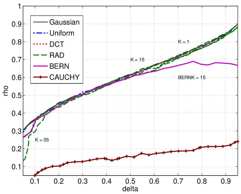
Next, we studied the effect of the measurement matrix construction on the performance of EM-GM-AMP in “sparse” mode with fixed . For this, we plotted EM-GM-AMP empirical PTCs for noiseless recovery of a length- BG signal under several types of measurement matrix : i.i.d , i.i.d Uniform , i.i.d centered Cauchy with scale , i.i.d Bernoulli1212 12 For the Bernoulli and BR matrices, we ensured that no two columns of a given realization were identical. (i.e., ) with , i.i.d zero-mean BR (i.e., ) with , and randomly row-sampled Discrete Cosine Transform (DCT). Figure 7 shows that the EM-GM-AMP PTC with i.i.d matrices also holds with the other i.i.d zero-mean sub-Gaussian examples (i.e., Uniform and BR with ). This is not surprising given that AMP itself has rigorous guarantees for i.i.d zero-mean sub-Gaussian matrices [5]. Figure 7 shows that the i.i.d- PTC is also preserved with randomly row-sampled DCT matrices, which is not surprising given AMP’s excellent empirical performance with many types of deterministic [27] even in the absence of theoretical guarantees. Figure 7 shows, however, that EM-GM-AMP’s PTC can degrade with non-zero-mean i.i.d matrices (as in the Bernoulli example) or with super-Gaussian i.i.d matrices (as in the BR example with sparsity rate and the Cauchy example). Surprisingly, the i.i.d- PTC is preserved by i.i.d-BR matrices with sparsity rate , even though is required for a BR matrix to be sub-Gaussian [28].
IV-B Noisy Sparse Signal Recovery
Figures 8–10 show NMSE for noisy recovery of BG, Bernoulli, and BR signals, respectively. To construct these plots, we fixed , , dB, and varied . Each data point represents NMSE averaged over realizations, where in each realization we drew an with i.i.d elements, an AWGN noise vector, and a random signal vector. For comparison, we show the performance of the proposed EM-GM-AMP (in “sparse” mode) for both MOS and versions, EM-BG-AMP, genie-tuned1313 13 We ran both OMP (using the implementation from http://sparselab.stanford.edu/OptimalTuning/code.htm) and SP under different sparsity assumptions, spaced uniformly from to , and reported the lowest NMSE among the results. Orthogonal Matching Pursuit (OMP) [29], genie-tuned13 Subspace Pursuit (SP) [30], Bayesian Compressive Sensing (BCS) [19], Sparse Bayesian Learning [18] (via the more robust T-MSBL [31]), de-biased genie-tuned1414 14 We ran SPGL1 in ‘BPDN’ mode: , for hypothesized tolerances , and reported the lowest NMSE among the results. LASSO (via SPGL1 [32]), and Smoothed- (SL0) [33]. All algorithms were run under the suggested defaults, with noise=small in T-MSBL.
For BG signals, Fig. 8 shows that EM-GM-AMP-MOS, EM-GM-AMP, and EM-BG-AMP together exhibit the best performance among the tested algorithms, reducing the breakpoint (i.e., the location of the knee in the NMSE curve, which represents a sort of phase transition) from down to , but also improving NMSE by dB relative to the next best algorithm, which was BCS. Relative to the other EM-AMP variants, MOS resulted in a slight degradation of performance for between and , but was otherwise identical. For Bernoulli signals, Fig. 9 shows much more significant gains for EM-GM-AMP-MOS, EM-GM-AMP and EM-BG-AMP over the other algorithms: the breakpoint was reduced from down to (and even with MOS), and the NMSE was reduced by dB relative to the next best algorithm, which was T-MSBL in this case. Finally, for BR signals, Fig. 10 shows a distinct advantage for EM-GM-AMP and EM-GM-AMP-MOS over the other algorithms, including EM-BG-AMP, due to the formers’ ability to accurately model the BR signal prior. In particular, for , EM-GM-AMP-MOS reduces the NMSE by dB relative to the best of the other algorithms (which was either EM-BG-AMP or T-MSBL depending on the value of ) and reduces the breakpoint from down to .


To investigate each algorithm’s robustness to AWGN, we plotted the NMSE attained in the recovery of BR signals with , , and as a function of SNR in Fig. 11, where each point represents an average over problem realizations, where in each realization we drew an with i.i.d elements, an AWGN noise vector, and a random signal vector. All algorithms were under the same conditions as those reported previously, except that T-MSBL used noise=small when dB and noise=mild when dB, as recommended in [34]. From Fig. 11, we see that the essential behavior observed in the fixed-SNR BR plot Fig. 10 holds over a wide range of SNRs. In particular, Fig. 11 shows that EM-GM-AMP and EM-GM-AMP-MOS yield significantly lower NMSE than all other algorithms over the full SNR range, while EM-BG-AMP and T-MSBL yield the second lowest NMSE (also matched by BCS for SNRs between and dB). Note, however, than T-MSBL must be given some knowledge about the true noise variance in order to perform well [34], unlike the proposed algorithms.

IV-C Heavy-Tailed Signal Recovery
In many applications of compressive sensing, the signal to be recovered is not perfectly sparse, but instead contains a few large coefficients and many small ones. While the literature often refers to such signals as “compressible,” there are many real-world signals that do not satisfy the technical definition of compressibility (see, e.g., [35]), and so we refer to such signals more generally as “heavy tailed.”
To investigate algorithm performance for these signals, we first consider an i.i.d Student’s-t signal, with prior pdf
| (82) |
under the (non-compressible) rate , which has been shown to be an excellent model for wavelet coefficients of natural images [35]. For such signals, Fig. 12 plots NMSE versus the number of measurements for fixed , dB, and an average of realizations, where in each realization we drew an with i.i.d elements, an AWGN noise vector, and a random signal vector. Figure 12 shows both variants of EM-GM-AMP (here run in ‘‘heavy-tailed’’ mode) outperforming all other algorithms under test.1515 15 In this experiment, we ran both OMP and SP under different sparsity hypotheses, spaced uniformly from to , and reported the lowest NMSE among the results. We have also verified (in experiments not shown here) that “heavy-tailed” EM-GM-AMP exhibits similarly good performance with other values of the Student’s-t rate parameter , as well as for i.i.d centered Cauchy signals.

To investigate the performance for positive heavy-tailed signals, we conducted a similar experiment using i.i.d log-normal , generated using the distribution
| (83) |
with location parameter and scale parameter . Figure 13 confirms the excellent performance of EM-GM-AMP-MOS, EM-GM-AMP, and EM-BG-AMP over all tested undersampling ratios . We postulate that, for signals known apriori to be positive, EM-GM-AMP’s performance could be further improved through the use of a prior with support restricted to the the positive reals, via a mixture of positively truncated Gaussians.

It may be interesting to notice that, with the perfectly sparse signals examined in Figs. 8–10, SL0 and SPGL1 performed relatively poorly, the relevance-vector-machine (RVM)-based approaches (i.e., BCS, T-MSBL) performed relatively well, and the greedy approaches (OMP and SP) performed in-between. With the heavy-tailed signals in Figs. 12–13, it is more difficult to see a consistent pattern. For example, with the Student’s-t signal, the greedy approaches performed the worse, the RVM approaches were in the middle, and SL0 and SPGL1 performed very well. But with the log-normal signal, the situation was very different: the greedy approaches performed very well, SPGL1 performed moderately well, but SL0 and the RVM approaches performed very poorly.
In conclusion, for all of the many signal types tested above, the best recovery performance came from EM-GM-AMP and its MOS variant. We attribute this behavior to EM-GM-AMP’s ability to tune itself to the signal (and in fact the realization) at hand.
IV-D Runtime and Complexity Scaling with
Next we investigated how complexity scales with signal length by evaluating the runtime of each algorithm on a typical personal computer. For this, we fixed , , dB and varied the signal length . Figure 14 shows the runtimes for noisy recovery of a Bernoulli-Rademacher signal, while Fig. 15 shows the corresponding NMSEs. In these plots, each datapoint represents an average over realizations. The algorithms that we tested are the same ones that we described earlier. However, to fairly evaluate runtime, we configured some a bit differently than before. In particular, for genie-tuned SPGL1, in order to yield a better runtime-vs-NMSE tradeoff, we reduced the tolerance grid (recall footnote 14) to and turned off debiasing. For OMP and SP, we used the fixed support size rather than searching for the size that minimizes NMSE over a grid of hypotheses, as before. Otherwise, all algorithms were run under the suggested defaults, with T-MSBL run under noise=small and EM-GM-AMP run in “sparse” mode.
The complexities of the proposed EM-GM-AMP methods are dominated by one matrix multiplication by and per iteration. Thus, when these matrix multiplications are explicitly implemented and is dense, the total complexity of EM-GM-AMP should scale as . This scaling is indeed visible in the runtime curves of Fig. 14. There, becomes since the ratio was fixed, and the horizontal axis plots on a logarithmic scale, so that this complexity scaling manifests, at sufficiently large values of , as a line with slope . Figure 14 confirms that genie-tuned SPGL1 also has the same complexity scaling, albeit with longer overall runtimes. Meanwhile, Fig. 14 shows T-MSBL, BCS, SL0, OMP, and SP exhibiting a complexity scaling of (under fixed and ), which results in orders-of-magnitude larger runtimes for long signals (e.g., ). With short signals (e.g., ), though, OMP, SP, SL0, and SPGL1 are faster than EM-GM-AMP. Finally, Fig. 15 verifies that, for most of the algorithms, the NMSEs are relatively insensitive to signal length when the undersampling ratio and sparsity ratio are both fixed, although the performance of EM-GM-AMP improves with (which is not surprising in light of AMP’s large-system-limit optimality properties [13]) and the performance of BCS degrades with .
Both the proposed EM-GM-AMP methods and SPGL1 can exploit the case where multiplication by and is implemented using a fast algorithm like the fast Fourier transform (FFT)1616 16 For our FFT-based experiments, we used the complex-valued versions of EM-BG-AMP, EM-GM-AMP, and SPGL1., which reduces the complexity to , and avoids the need to store in memory—a potentially serious problem when is large. The dashed lines in Figs. 14–15 (labeled “fft”) show the average runtime and NMSE of the proposed algorithms and SPGL1 in case that was a randomly row-sampled FFT. As expected, the runtimes are dramatically reduced. While EM-BG-AMP retains its place as the fastest algorithm, SPGL1 now runs faster than EM-GM-AMP (at the cost of dB higher NMSE). The MOS version of EM-GM-AMP yields slightly better NMSE, but takes times as long to run as the fixed- version.


IV-E Example: Compressive Recovery of Audio
As a practical example, we experimented with the recovery of an audio signal from compressed measurements. The full length- audio signal was first partitioned into blocks of length . Noiseless compressed measurements were then collected using samples per block. Rather than reconstructing directly from , we first reconstructed1717 17 Although one could exploit additional structure among the multiple-timestep coefficients for improved recovery (e.g., sparsity clustering in the time and/or frequency dimensions, as well as amplitude correlation in those dimensions) as demonstrated in [36], such techniques are outside the scope of this paper. the transform coefficients , using the (orthogonal) discrete cosine transform (DCT) , and later reconstructed via . Our effective sparse-signal model can thus be written as with . We experimented with two types of measurement matrix : i.i.d zero-mean Gaussian and random selection (i.e., containing rows of the identity matrix selected uniformly at random), noting that the latter allows a fast implementation of and . Table III shows the resulting time-averaged NMSE, i.e., , and total runtime achieved by the previously described algorithms at block lengths , which correspond to blocks, respectively. The numbers reported in the table represent an average over realizations of . For these experiments, we configured the algorithms as described in Section IV-C for the heavy-tailed experiment except that, for genie-SPGL1, rather than using , we used for the tolerance grid (recall footnote 14) because we found that this value minimized TNMSE and, for T-MSBL, we used the setting prune_gamma = as recommended in a personal correspondence with the author. For certain combinations of algorithm and blocklength, excessive runtimes prevented us from carrying out the experiment, and thus no result appears in the table.
Table III shows that, for this audio experiment, the EM-GM-AMP methods and SL0 performed best in terms of TNMSE. As in the synthetic examples presented earlier, we attribute EM-GM-AMP’s excellent TNMSE to its ability to tune itself to whatever signal is at hand. As for SL0’s excellent TNMSE, we reason that it had the good fortune of being particularly well-tuned to this audio signal, given that it performed relatively poorly with the signal types used for Figs. 8–11 and Fig. 13. From the runtimes reported in Table III, we see that, with i.i.d Gaussian and the shortest block length (), genie-OMP is by far the fastest, whereas the EM-GM-AMP methods are the slowest. But, as the block length grows, the EM-GM-AMP methods achieve better and better runtimes as a consequence of their excellent complexity scaling, and eventually EM-BG-AMP and fixed- EM-GM-AMP become the two fastest algorithms under test (as shown with i.i.d Gaussian at ). For this audio example, the large-block regime may be the more important, because that is where all algorithms give their smallest TNMSE. Next, looking at the runtimes under random-selection , we see dramatic speed improvements for the EM-GM-AMP methods and SPGL1, which were all able to leverage Matlab’s fast DCT. In fact, the total runtimes of these four algorithms decrease as is increased from to . We conclude by noting that EM-BG-AMP (at with random selection ) achieves the fastest runtime in the entire table while yielding a TNMSE that is within dB of the best value in the entire table. Meanwhile, fixed- EM-GM-AMP (at with random selection ) gives TNMSE only dB away from the best in the entire table with a runtime of only about twice the best in the entire table. Finally, the best TNMSEs in the entire table are achieved by EM-GM-AMP-MOS (at ), which takes times as long to run as its fixed- counterpart.
| TNMSE | time | TNMSE | time | TNMSE | time | TNMSE | time | ||
|---|---|---|---|---|---|---|---|---|---|
| i.i.d Gaussian | EM-GM-AMP-MOS | -17.3 | 468.9 | -18.3 | 487.2 | -21.0 | 967.9 | -21.8 | 2543 |
| EM-GM-AMP | -16.9 | 159.2 | -18.0 | 213.2 | -20.7 | 434.0 | -21.4 | 1129 | |
| EM-BG-AMP | -15.9 | 115.2 | -17.0 | 174.1 | -19.4 | 430.2 | -20.0 | 1116 | |
| SL0 | -16.8 | 41.6 | -17.9 | 128.5 | -20.6 | 629.0 | -21.3 | 2739 | |
| genie SPGL1 | -14.3 | 90.9 | -16.2 | 200.6 | -18.6 | 514.3 | -19.5 | 1568 | |
| BCS | -15.0 | 67.5 | -15.8 | 149.1 | -18.4 | 428.0 | -18.8 | 2295 | |
| T-MSBL | -16.3 | 1.2e4 | – | – | – | – | – | – | |
| genie OMP | -13.9 | 20.1 | -14.9 | 109.9 | -17.6 | 527.0 | – | – | |
| genie SP | -14.5 | 87.7 | -15.5 | 305.9 | -18.0 | 1331 | – | – | |
| random selection | EM-GM-AMP-MOS | -16.6 | 233.0 | -17.5 | 136.1 | -20.5 | 109.6 | -21.6 | 93.9 |
| EM-GM-AMP | -16.7 | 56.1 | -17.7 | 43.7 | -20.5 | 38.0 | -21.5 | 37.8 | |
| EM-BG-AMP | -16.2 | 29.6 | -17.2 | 22.3 | -19.7 | 19.4 | -20.5 | 18.0 | |
| SL0 | -16.7 | 35.7 | -17.6 | 119.5 | -20.4 | 597.8 | -21.2 | 2739 | |
| genie SPGL1 | -14.0 | 34.4 | -15.9 | 24.5 | -18.4 | 21.7 | -19.7 | 19.6 | |
| BCS | -15.5 | 60.5 | -16.1 | 126.2 | -19.4 | 373.8 | -20.2 | 2295 | |
| T-MSBL | -15.5 | 1.2e4 | – | – | – | – | – | – | |
| genie OMP | -15.1 | 20.1 | -15.7 | 106.8 | -18.9 | 506.0 | – | – | |
| genie SP | -15.2 | 104.5 | -16.1 | 395.3 | -18.7 | 1808 | – | – | |
V Conclusions
Those interested in practical compressive sensing face the daunting task of choosing among literally hundreds of signal reconstruction algorithms (see, e.g., [37]). In testing these algorithms, they are likely to find that some work very well with particular signal classes, but not with others. They are also likely to get frustrated by those algorithms that require the tuning of many parameters. Finally, they are likely to find that some of the algorithms that are commonly regarded as “very fast” are actually very slow in high-dimensional problems. Meanwhile, those familiar with the theory of compressive sensing know that the workhorse LASSO is nearly minimax optimal, and that its phase transition curve is robust to the nonzero-coefficient distribution of sparse signals. However, they also know that, for most signal classes, there is a large gap between the MSE performance of LASSO and that of the MMSE estimator derived under full knowledge of the signal and noise statistics [11]. Thus, they may wonder whether there is a way to close this gap by designing a signal reconstruction algorithm that both learns and exploits the signal and noise statistics.
With these considerations in mind, we proposed an empirical Bayesian approach to compressive signal recovery that merges two powerful inference frameworks: expectation maximization (EM) and approximate message passing (AMP). We then demonstrated—through a detailed numerical study—that our approach, when used with a flexible Gaussian-mixture signal prior, achieves a state-of-the-art combination of reconstruction error and runtime on a very wide range of signal and matrix types in the high-dimensional regime. However, certain non-zero-mean and super-Gaussian sensing matrices give our AMP-based method trouble. Making AMP robust to these matrices remains a topic of importance for future research.
References
- [1] J. P. Vila and P. Schniter, “An empirical-Bayes approach to compressive sensing via approximate message passing.” presented at the Duke Workshop on Sensing and Analysis of High-Dimensional Data, (Durham, NC), July 2011.
- [2] J. P. Vila and P. Schniter, “Expectation-maximization Bernoulli-Gaussian approximate message passing,” in Proc. Asilomar Conf. Signals Syst. Comput., (Pacific Grove, CA), pp. 799–803, Nov. 2011.
- [3] J. P. Vila and P. Schniter, “Expectation-maximization Gaussian-mixture approximate message passing,” in Proc. Conf. Inform. Science & Syst., (Princeton, NJ), pp. 1–6, Mar. 2012.
- [4] Y. C. Eldar and G. Kutyniok, Compressed Sensing: Theory and Applications. New York: Cambridge Univ. Press, 2012.
- [5] M. Bayati, M. Lelarge, and A. Montanari, “Universality in polytope phase transitions and iterative algorithms,” in Proc. IEEE Int. Symp. Inform. Thy., (Boston, Ma), pp. 1–5, June 2012. (see also arXiv:1207.7321).
- [6] R. Tibshirani, “Regression shrinkage and selection via the lasso,” J. Roy. Statist. Soc. B, vol. 58, no. 1, pp. 267 – 288, 1996.
- [7] S. S. Chen, D. L. Donoho, and M. A. Saunders, “Atomic decomposition by basis pursuit,” SIAM J. Scientific Comput., vol. 20, no. 1, pp. 33–61, 1998.
- [8] D. L. Donoho and J. Tanner, “Observed universality of phase transitions in high-dimensional geometry, with implications for modern data analysis and signal processing,” Phil. Trans. Royal Soc. A, vol. 367, no. 1906, pp. 4273–4293, 2009.
- [9] D. L. Donoho, A. Maleki, and A. Montanari, “The noise-sensitivity phase transition in compressed sensing,” arXiv:1004.1218, Apr. 2010.
- [10] D. L. Donoho, A. Maleki, and A. Montanari, “Message passing algorithms for compressed sensing,” Proc. Nat. Acad. Sci., vol. 106, pp. 18914–18919, Nov. 2009.
- [11] Y. Wu and S. Verdú, “Optimal phase transitions in compressed sensing,” IEEE Trans. Inform. Theory, vol. 58, pp. 6241–6263, Oct. 2012.
- [12] D. L. Donoho, A. Maleki, and A. Montanari, “Message passing algorithms for compressed sensing: I. Motivation and construction,” in Proc. Inform. Theory Workshop, (Cairo, Egypt), pp. 1–5, Jan. 2010.
- [13] M. Bayati and A. Montanari, “The dynamics of message passing on dense graphs, with applications to compressed sensing,” IEEE Trans. Inform. Theory, vol. 57, pp. 764–785, Feb. 2011.
- [14] S. Rangan, “Generalized approximate message passing for estimation with random linear mixing,” in Proc. IEEE Int. Symp. Inform. Thy., (Saint Petersburg, Russia), Aug. 2011. (Full version at arXiv:1010.5141).
- [15] A. Dempster, N. M. Laird, and D. B. Rubin, “Maximum-likelihood from incomplete data via the EM algorithm,” J. Roy. Statist. Soc., vol. 39, pp. 1–17, 1977.
- [16] B. Efron, Large-Scale Inference: Empirical Bayes Methods for Estimation, Testing, and Prediction. New York: Cambridge University Press, 2010.
- [17] M. E. Tipping, “Sparse Bayesian learning and the relevance vector machine,” J. Mach. Learn. Res., vol. 1, pp. 211–244, 2001.
- [18] D. P. Wipf and B. D. Rao, “Sparse Bayesian learning for basis selection,” IEEE Trans. Signal Process., vol. 52, pp. 2153–2164, Aug. 2004.
- [19] S. Ji, Y. Xue, and L. Carin, “Bayesian compressive sensing,” IEEE Trans. Signal Process., vol. 56, pp. 2346–2356, June 2008.
- [20] U. S. Kamilov, S. Rangan, A. K. Fletcher, and M. Unser, “Approximate message passing with consistent parameter estimation and applications to sparse learning,” in Proc. Neural Inform. Process. Syst. Conf., (Lake Tahoe, NV), Dec. 2012. (Full version at arXiv:1207.3859).
- [21] U. S. Kamilov, A. Bourquard, A. Amini, and M. Unser, “One-bit measurements with adaptive thresholds,” IEEE Signal Process. Lett., vol. 19, pp. 607–610, Oct. 2012.
- [22] C. F. J. Wu, “On the convergence properties of the EM algorithm,” Ann. Statist., vol. 11, no. 1, pp. 95–103, 1983.
- [23] R. Neal and G. Hinton, “A view of the EM algorithm that justifies incremental, sparse, and other variants,” in Learning in Graphical Models (M. I. Jordan, ed.), pp. 355–368, MIT Press, 1999.
- [24] C. M. Bishop, Pattern Recognition and Machine Learning. New York: Springer, 2007.
- [25] P. Stoica and Y. Selén, “Model-order selection: A review of information criterion rules,” IEEE Signal Process. Mag., vol. 21, pp. 36–47, July 2004.
- [26] A. Beck and M. Teboulle, “A fast iterative shrinkage-thresholding algorithm for linear inverse problems,” SIAM J. Imag. Sci., vol. 2, no. 1, pp. 183–202, 2009.
- [27] H. Monajemi, S. Jafarpour, M. Gavish, Stat 330/CME 362 Collaboration, and D. L. Donoho, “Deterministic matrices matching the compressed sensing phase transitions of Gaussian random matrices,” Proc. Nat. Acad. Sci., vol. 110, pp. 1181–1186, Jan. 2013.
- [28] V. V. Buldygin and Y. V. Kozachenko, Metric Characterization of Random Variables and Random Processes. Providence, RI: Americal Mathematical Society, 2000.
- [29] Y. C. Pati, R. Rezaiifar, and P. S. Krishnaprasad, “Orthogonal matching pursuit: Recursive function approximation with applications to wavelet decomposition,” in Proc. Asilomar Conf. Signals Syst. Comput., (Pacific Grove, CA), pp. 40–44, 1993.
- [30] W. Dai and O. Milenkovic, “Subspace pursuit for compressive sensing reconstruction,” IEEE Trans. Inform. Theory, vol. 55, pp. 2230–2249, Mar. 2009.
- [31] Z. Zhang and B. D. Rao, “Sparse signal recovery with temporally correlated source vectors using sparse Bayesian learning,” IEEE J. Sel. Topics Signal Process., vol. 5, pp. 912–926, Sept. 2011.
- [32] E. van den Berg and M. P. Friedlander, “Probing the Pareto frontier for basis pursuit solutions,” SIAM J. Scientific Comput., vol. 31, no. 2, pp. 890–912, 2008.
- [33] H. Mohimani, M. Babaie-Zadeh, and C. Jutten, “A fast approach for overcomplete sparse decomposition based on smoothed norm,” IEEE Trans. Signal Process., vol. 57, pp. 289–301, Jan. 2009.
- [34] Z. Zhang, “Master the usage of T-MSBL in 3 minutes,” tech. rep., Univ. of California, San Diego, Nov. 2011.
- [35] V. Cevher, “Learning with compressible priors,” in Proc. Neural Inform. Process. Syst. Conf., (Vancouver, B.C.), pp. 261–269, Dec. 2009.
- [36] J. Ziniel, S. Rangan, and P. Schniter, “A generalized framework for learning and recovery of structured sparse signals,” in Proc. IEEE Workshop Statist. Signal Process., (Ann Arbor, MI), pp. 325–328, Aug. 2012.
- [37]
“Compressive sensing resources: References and software,”
http://dsp.rice.edu/cs.
![[Uncaptioned image]](1207.3107v3/jeremy.png) |
Jeremy Vila received the B.S. degree in Electrical and Computer Engineering from the Ohio State University in 2010. He is currently a Ph.D. student in the Information Processing Systems Lab in the Department of Electrical and Computer Engineering at OSU. His primary research interests include compressive sensing, statistical signal processing, and machine learning. |
![[Uncaptioned image]](1207.3107v3/phil.png) |
Philip Schniter received the B.S. and M.S. degrees in Electrical Engineering from the University of Illinois at Urbana-Champaign in 1992 and 1993, respectively, and the Ph.D. degree in Electrical Engineering from Cornell University in Ithaca, NY, in 2000. From 1993 to 1996 he was employed by Tektronix Inc. in Beaverton, OR as a systems engineer. After receiving the Ph.D. degree, he joined the Department of Electrical and Computer Engineering at The Ohio State University, Columbus, where he is currently a Professor and a member of the Information Processing Systems (IPS) Lab. In 2008-2009 he was a visiting professor at Eurecom, Sophia Antipolis, France, and Supélec, Gif-sur-Yvette, France. In 2003, Dr. Schniter received the National Science Foundation CAREER Award. His areas of interest currently include statistical signal processing, wireless communications and networks, and machine learning. |