Graham Higman’s lectures on januarials

Graham Higman gave the lectures on which this article is based, in Oxford in 2001. They are likely to have been the final lectures he gave; he died in April 2008, at the age of 91. He introduced them with the quotes from W.B. Yeats reproduced above, and described the work in preparing them as “justifying my old age” and “keeping me relatively sane.” The second author attended the lectures, and the first author remembers Higman’s work on related topics some years earlier; this account is developed from recollections and from notes taken at the time. As such, any errors are ours, and the presentation and the proofs offered may not be as Higman had in mind. At various points, and as indicated, we have extended Higman’s treatment; we also include some of our own observations in an afterword.

Januarials, which we will define in Section 2, are 2-complexes with two distinguished faces, that result from embedding coset graphs for the actions of triangle groups into compact orientable surfaces. They can be viewed as being assembled from two sub-surfaces (essentially those two distinguished faces); we give appropriate definitions and tools to explore the complexity of this assembly in Section 3. In Section 4 we give sufficient conditions for actions of $\hbox{\rm PSL}(2,p)$ on projective lines to give rise to januarials. This leads to a number of examples presented in Section 5. Finally Section 6, our afterword, contains some remarks on the coset graph appearing in Norman Blamey’s 1984 portrait of Higman, and some further examples of januarials.

It appears that Higman’s study of januarials was sparked by his work on Hurwitz groups, which are non-trivial finite quotients of the $(2,3,7)$-triangle group. Higman used coset diagrams to show that for all sufficiently large $n$, the alternating group $\textup{Alt}(n)$ is a Hurwitz group, and his work was taken further by the first author to determine exactly which $\textup{Alt}(n)$ are Hurwitz, in [1].

Funding. This work was partially supported by the New Zealand Marsden Fund [grant UOA1015] to MDEC; and the United States National Sciences Foundation [grant DMS–1101651] to TRR; and the Simons Foundation [collaboration grant 208567] to TRR.

Acknowledgements. We are grateful to Martin Bridson, Harald Helfgott and Peter Neumann for encouragement and guidance in the writing of this account, and to Stephen Blamey and Sam Howison (Chairman of the Oxford Mathematical Institute) for permission to reproduce Norman Blamey’s portrait of Graham Higman in Figure 11. We also thank the referee for carefully reading this article and making some very helpful suggestions.

Suppose $S$ is a set endowed with an action $s\mapsto s^{g}$ by a group $G$, and $A$ is a generating set for $G$. Define $\Gamma$ to be the graph with vertex set $S,$ and with an oriented edge labelled by $a\in A$ (called an $a$-edge) from vertex $u$ to vertex $v$ whenever $u^{a}=v$. We will be concerned with situations where $G$ acts transitively on $S$, so that $\Gamma$ is connected. In that event we can identify $S$ with the right cosets $\left\{\,Hg:g\in G\,\right\}$ of the stabiliser $H=G_{s}=\hbox{\rm Stab}_{G}(s)$ of any particular $s\in S$, and for this reason, $\Gamma$ is known as a coset graph or Schreier graph, or sometimes coset diagram, for the action of $G$ on $S$ with respect to $A$. When the action of $G$ on $S$ is also regular, we can identify $S$ with the underlying set of $G$, in which case $\Gamma$ is the Cayley graph of $G$ with respect to $A$.

Paths in the coset graph may be labelled with words on the generating set $A$ (which can be thought of as an alphabet). Suppose that a word $w$ on $A^{\pm 1}$ represents $g\in G$, and that $s\in S$. Let $\gamma$ be the path in $\Gamma$ obtained by concatenating the unique edge-paths in $\Gamma$ from $s^{g^{i}}$ to $s^{g^{i+1}}$, for each $i\in\mathbb{Z}$, along which one reads $w$. This tours an orbit of $\langle g\rangle$ and is a (closed) circuit precisely when that orbit is finite. There is one such path for each orbit.

A map is a 2-cell embedding of a connected (multi)graph in some closed surface, with its faces (the components of the complement of the graph in the surface) being homeomorphic to open disks in $\mathbb{R}^{2}$. Examples include triangulations and quadrangulations of the torus, and the Platonic solids (which may be viewed as highly symmetric maps on the sphere), with all vertices having the same valence and all faces having the same size.

A januarial is a special instance of a map constructed from embedding a coset graph for an action of the the $(2,k,l)$ triangle group

with $A=\left\{x,y\right\}$. Because $x^{2}=1$, the $x$-edges in such a coset graph $\Gamma$ coming from non-trivial cycles of $x$ occur in pairs: whenever there is an $x$-edge from $u$ to $v$, there is an $x$-edge from $v$ to $u$. We may identify each such pair, so as to leave an unoriented $x$-edge between $u$ and $v$. Then for each fixed point $s$ of $x$, we attach a 2-cell (which we will call an $x$-monogon) along the $x$-edge which forms a loop at $s$. Similarly, for each orbit of $\langle y\rangle$, we attach a polygon (which we call a $y$-face) along the path $\gamma$ given by $\langle y\rangle$ as described above. This gives a 2-complex, many examples of which appear in this article; see Figures 1, 2, 6, 7, 8, 9, and 10. These and similar figures can be displayed without labels on the edges, because we may shade the $y$-faces so that $y$-edges are identifiable as those in the boundaries of $y$-faces, while all the remaining edges are $x$-edges. We need not indicate orientations on the edges: the $x$-edges for the reason given above, and the $y$-edges because we may adopt a convention that all $y$-edges are oriented anti-clockwise around the corresponding $y$-faces. Note that the length (the number of sides) of each $y$-face divides $k$.

Next, attach a polygon (which we call an $xy$-face) around each orbit of $\langle xy\rangle$. As shown by the following lemma, the resulting 2-complex $J$ is homeomorphic to a closed orientable surface. We may call the corresponding embedding of $\Gamma$ an $m$-face map, where $m$ is the number of orbits of $\langle xy\rangle$.

A januarial (and more precisely, a $k$-januarial) is the instance when $m=2$ and the orbits of $\langle xy\rangle$ have the same size $\left|\,S\right|/2$. Two examples of $3$-januarials are given in Figure 3.

Higman gave a notion of topological complexity which we call simple type below. It concerns how a januarial $J$ is assembled from the subspaces $S_{1}$ and $S_{2}$ that are the closures of its two $xy$-faces. He recognised that some januarials are beyond the scope of this notion; indeed, he made some ad hoc calculations for the examples in Figures 8 and 10 which show as much. Accordingly, below, we define a more general notion which we call type, which applies to all januarials, and we explain how to calculate it in general.

Topological features of $J$, $S_{1}$ and $S_{2}$ come into clearer focus when we collapse each $x$-monogon and each $y$-face in $J$ to a point. Any two $y$-faces in a januarial are disjoint. The same is true of any two $x$-monogons. And an $x$-monogon can only meet a $y$-face at a single vertex. So these collapses do not change the homeomorphism types of $J$, $S_{1}$ or $S_{2}$.

Let $\Gamma$ be the 1-skeleton of $J$ — that is, the coset graph. Let $\overline{J}$, $\overline{S_{1}}$, $\overline{S_{2}}$ and $\overline{\Gamma}$ be the images of $J$, $S_{1}$, $S_{2}$ and $\Gamma$ under these collapses. We call $\overline{\Gamma}$ a companion graph. Then $\overline{J}=\overline{S_{1}}\cup\overline{S_{2}}$ is a closed surface obtained by some identification of $\overline{S_{1}}$ and $\overline{S_{2}}$ along their boundaries. Taking another perspective, $\overline{J}$ is the result of adding two faces to $\overline{\Gamma}$, via attaching maps $\rho_{1}$ and $\rho_{2}$ induced by the maps that attach the $xy$-faces to $\Gamma$.

Examples of such $\Gamma$ and $\overline{\Gamma}$ appear in Figures 1, 2, 7, 8, 10, 12, and 13. Each one is drawn in such a way that the cyclic order in which edges emanate from vertices agrees with that in which $x$-edges meet $y$-faces in $\Gamma$. So, as the $y$-edges in $\Gamma$ are oriented anti-clockwise around the $y$-faces, one can read off $\rho_{i}$ by following successive edges in $\overline{\Gamma}$ in such a way that on arriving at a vertex, one exits along the right-most of all the remaining edges (except if the vertex has valence one, in which case one exits along the edge by which one arrived).

As $\langle xy\rangle$ yields exactly two orbits when acting on $S$, together $\rho_{1}$ and $\rho_{2}$ traverse each edge in $\overline{\Gamma}$ twice, once in each direction. The edges comprising the subgraph $\mathcal{G}:=\overline{S_{1}}\cap\overline{S_{2}}$, shown in blue in the figures, are traversed by $\rho_{1}$ in one direction and $\rho_{2}$ in the other. Those traversed by $\rho_{1}$ (resp. $\rho_{2}$) in both directions are shown in red (resp. green).

The collapses carrying $J$ to $\overline{J}$ leave only the two $xy$-faces, those $x$-edges which are not loops, and one vertex for each $y$-face in $J$. These collapses do not alter the Euler characteristic. Since $J$ is a closed orientable surface, we find that the genus of $J$ is readily calculated as follows.

For example, this is $6-6=0$ in the left-hand example of Figure 3 and is $8-6=2$ in the right-hand example, giving genera $0$ and $1$, respectively.

Now we turn to genera associated to $S_{1}$ and $S_{2}$, or their images $\overline{S_{1}}$ and $\overline{S_{2}}$. Defining these requires care, since $\overline{S_{1}}$ and $\overline{S_{2}}$ may fail to be sub-surfaces of $\overline{J}$ (and likewise $S_{1}$ and $S_{2}$ fail to be sub-surfaces of $J$): they are closed surfaces from which the interiors of some collection of discs have been removed, but the boundaries of those discs need not be disjoint. (Figures 8 and 10 provide such examples.) But if we take a small closed neighbourhood $R_{i}$ of $\overline{S_{i}}$ in $\overline{J}$, we get a genuine sub-surface which serves as a suitable proxy:

We define the type of $J$ to be the pair $((h_{1},g_{1}),(h_{2},g_{2}))$, where $g_{i}$ and $h_{i}$ are the genus of $R_{i}$ and the number of connected components of the boundary of $R_{i}$ respectively, for $i=1,2$. We will not distinguish between types $((h_{1},g_{1}),(h_{2},g_{2}))$ and $((h_{2},g_{2}),(h_{1},g_{1}))$.

The most straightforward way in which $R_{1}$ and $R_{2}$ can be assembled to make $\overline{J}$ occurs when $R_{1}\cap R_{2}$ is a disjoint union of $h$ annuli, where $h=h_{1}=h_{2}$, or in other words, when $\overline{J}$ is homeomorphic to a join of $R_{1}$ and $R_{2}$ in which the boundary components are paired off and identified. In this case, we say that the januarial $J$ is of simple type $(h,g_{1},g_{2})$. We do not distinguish between the simple types $(h,g_{1},g_{2})$ and $(h,g_{2},g_{1})$.

Maps in which the graph is embedded in a suitably non-pathological manner (for instance as a subgraph of the $1$-skeleton of a finite cellulation of the surface) have the property that a small neighbourhood is a disjoint union of annuli if and only if the graph is a collection of disjoint simple circuits. So, as $R_{1}\cap R_{2}$ is a small neighbourhood of $\mathcal{G}$, one can recognise simple type from the graph $\overline{\Gamma}\,$:

The genus of a januarial $J$ (equivalently, of $\overline{J}$) of simple type is present in the data $(h,g_{1},g_{2})$. When the handles (that is, the $h$ annuli from $R_{1}\cap R_{2}$) that connect ${R_{1}}$ and ${R_{2}}$ are severed one-by-one, the genus falls by $1$ each time, until we only have one handle connecting ${R_{1}}$ and ${R_{2}}$, and hence a surface of genus $g_{1}+g_{2}$. Since $J$ has $h$ handles to begin with, this gives the following:

Figures 1, 2, 7 and 12 show examples of coset graphs which give januarials of simple type, and Figures 8, 10 and 13 show examples which give januarials that are not of simple type. In each case, the caption indicates the genus of the januarial and the details of the type. The genus of the januarial can be established in each case via an Euler characteristic calculation (as per Lemma 3.4 for those of simple type).

For the examples of simple type, $h$ is immediately evident from the companion graph $\overline{\Gamma}$ on account of Lemma 3.3. For those not of simple type, our next lemma gives a means of identifying $h_{1}$ and $h_{2}$ from $\overline{\Gamma}$. Examples of partitions of $\mathcal{G}$ into circuits in the sense of this lemma can be seen in Figures 8, 10 and 13.

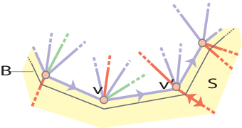
Given $h_{i}$ (for $i=1$ or $2$), one can determine $g_{i}$ from $\overline{\Gamma}$ via the following observation:

References

- [1] M.D.E. Conder, Generators for alternating and symmetric groups, J. London Math. Soc (2) 22, 1980, 75–86.
- [2] H.S.M. Coxeter, The abstract groups , Trans. Amer. Math. Soc. 45 (1939), 73–150.
- [3] H.S.M. Coxeter and W.O.J. Moser, Generators and Relations for Discrete Groups, 4th ed., Springer Berlin (1980).
- [4] B. Huppert, Endliche Gruppen. I. Die Grundlehren der Mathematischen Wissenschaften, Band 134, Springer-Verlag, Berlin-New York 1967 xii+793 pp.
- [5] G.A. Jones and J.S. Thornton, Automorphisms and congruence subgroups of the extended modular group, J. London Math. Soc. (2) 34 (1986), 26–40.
- [6] A.M. Macbeath, Generators of the linear fractional groups, in Number Theory, Proc. Symposia in Pure Mathematics 12 (American Mathematical Society, Providence, R.I., 1969), pp. 14-32.