Mean-Field Analysis of Spinor Bosons in Optical Superlattices
Abstract
We study the ground-state phase diagram of spinless and spin-1 bosons in optical superlattices using a Bose-Hubbard Hamiltonian that includes spin-dependent interactions. We decouple the unit cells of the superlattice via a mean-field approach and take into account the dynamics within the unit cell exactly. The system supports Mott-insulating as well as superfluid phases. The transitions between these phases are second-order for spinless bosons and second- or first-order for spin-1 bosons. Anti-ferromagnetic interactions energetically penalize high-spin configurations and elongate all Mott lobes, especially the ones corresponding to an even atom number on each lattice site. We find that the quadratic Zeeman effect lifts the degeneracy between different polar superfluid phases leading to additional metastable phases and first-order phase transitions. Finally, we show that an energy offset between the two sites of the unit cell induces a staircase of single-atom tunneling resonances which surprisingly survives well into the superfluid regime.
pacs
03.75.Lm, 67.85.Fg, 03.75.Mn, 05.30.RtI Introduction
Ultracold atom experiments offer the unique opportunity to study quantum many-body effects in an extremely clean and well-controlled environment. In contrast to most condensed matter systems they are characterized by the absence of disorder and other imperfections and are highly controllable. This is why they have been proposed as quantum simulators [1, 2, 3].
One of the most prominent achievements in this direction has been the observation of the quantum phase transition between a Mott insulating and a superfluid phases of ultracold atoms in an optical lattice [4, 5, 6]. In this situation, the ratio of the tunneling strength between the lattice sites and the on-site interaction determines the qualitative behavior of a quantum gas. If the on-site interaction dominates and the filling is commensurate the quantum gas is in the Mott-insulating phase. On the contrary, if the tunneling amplitude is sufficiently large the system becomes superfluid.
For atoms trapped in a magneto-optical trap the spin degree of freedom is frozen and the atoms become effectively spinless. If, however, the quantum gas is trapped by purely optical means, the atoms keep their spin degree of freedom and the order parameter describing the superfluid phase becomes a spinor. These systems were first studied in Refs. [7, 8] and recently reviewed in Ref. [9].
Due to their spin-dependent interactions ultracold spinor quantum gases in optical lattices offer the possibility to model mesoscopic magnetism [26]. They are well described by the Bose-Hubbard model, but the spin-dependent effects alter the system in a qualitative and quantitative way [10, 11, 12, 13, 14, 15]. The phase boundaries between superfluid and a Mott-insulating phases are shifted, and for certain atom-configurations the phase transition is no longer second- but first-order. This is a consequence of the additional spin-dependent on-site interaction. If this interaction is anti-ferromagnetic, atomic singlets are energetically favored and the Mott-insulating phase is stable in some parameter ranges where the system is superfluid for spinless atoms. The occurrence of first-order phase transitions enables metastable phases and the system shows hysteretic behavior.

In this paper we investigate ultracold bosons loaded into optical superlattices. These systems have already been studied theoretically [16, 17] and experimentally [18, 19, 20, 21]. We take into account the dynamics in the double wells exactly and include the tunneling between neighboring unit cells via a mean-field ansatz. The system supports Mott-insulating phases as well as superfluid phases [22, 23]. The former are characterized by a fixed number of atoms per unit cell. For spin-1 atoms we find that some of the phase transitions become first order similar to the case of usual period-1 lattices [14].
We include the effects of magnetic fields by using an effective Hamiltonian which includes a quadratic Zeeman shift. For anti-ferromagnetic interactions magnetic fields break the degeneracy between different polar superfluid phases. This leads to new classes of metastable phases and changes the phase boundaries significantly. In the ferromagnetic case magnetic fields cause first-order phase transitions and metastable phases. These results apply to spin-1 atoms in superlattices as well as in usual lattices.
Finally, we examine single-atom tunneling resonances in superlattices. These are known from isolated double-well potentials [24, 25, 26] and are generalized to superlattices in this work.
The remainder of this paper is organized as follows. In Sec. II we introduce the mean-field Hamiltonian for spinless bosons in optical superlattices. We discuss methods to treat this Hamiltonian and present the phase diagram in Sec. II.1. Section II.2 treats the phenomenon of single-atom resonances for spinless atoms in optical superlattices. In Sec. III we generalize the Bose-Hubbard Hamiltonian of Sec. II by including spin-dependent interactions. In Sec. III.1 the phase diagram of spin-1 atoms is examined. We discuss the novel aspects due to the spinor nature of the order parameter and point out differences in the single-atom resonances. Finally, we include magnetic fields in Sec. III.2 which enhance spin-dependent effects and lead to additional metastable phases.
II Spinless Bosons
Optical lattices are arrays of weakly connected optical micro-traps created by interfering counter-propagating laser beams. When the lattice is superimposed with a second standing laser beam with half the wavelength an optical superlattice is created (see Fig. 1). The unit cell of a period-2 superlattice is a double-well potential [18, 19, 20, 21].
Ultracold bosons in sufficiently deep optical lattices can be described by the Bose-Hubbard Hamiltonian [5, 27]. Here we examine the physics of bosonic atoms in optical superlattices when the overall atom density is chosen such that there are a few atoms per double well. If one neglects tunneling between neighboring unit cells the atoms in each unit cell can be described by the Hamiltonian
| (1) | |||||
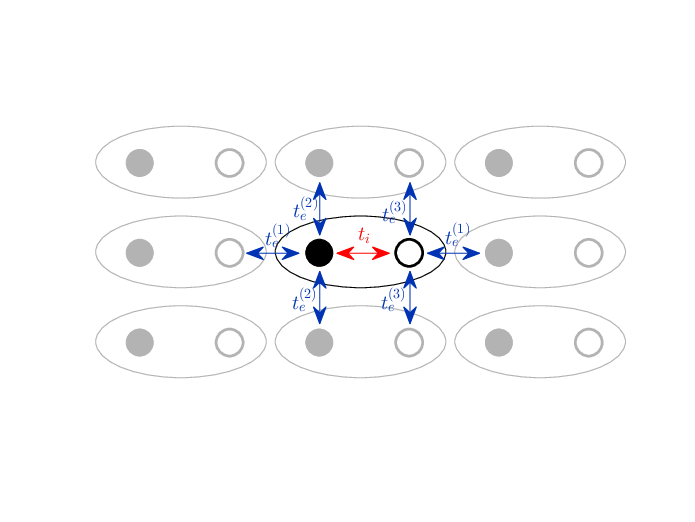
where and are bosonic annihilation (creation) operators for atoms in the left or right well, is the atom number operator at the left (right) site. is the on-site interaction and is the tunneling strength between the sites of the double well. The energy offset between the sites is given by and the chemical potential is (see Fig. 1). The parameters can be tuned by changing the intensity and the phase difference between the counter-propagating laser beams; it is possible to tune the system from the regime of strong tunneling () to the regime of weak tunneling ().
The Hamiltonian of an array of connected double-well potentials includes tunneling between neighboring unit cells. We choose the configuration as shown in Fig. 2 where there are in general three different inter-well tunneling amplitudes, , and . It turns out that the our results depend only weakly on the differences among the inter-well tunneling amplitudes. This is why we will assume .
Within the mean-field approximation which has been developed in Refs. [28, 22], our Hamiltonian reads
| (2) | |||||
where we introduced the mean-field parameters , , and for 2D lattices and for 3D lattices. The Hamiltonian treats the internal degrees of freedom of each unit cell exactly and approximates the tunneling between the unit cells via a mean-field ansatz. This approach is expected to give satisfactory results if the tunneling inside the unit cells is stronger than the tunneling between the unit cells (i.e., ), otherwise correlations between neighboring double wells would be stronger than correlations within the double wells and should not be neglected.

The system is in the Mott-insulating phase if and in the superfluid phase if . In the latter case the number of superfluid atoms and on the left and right site is given by .
There are several possibilities to treat the Hamiltonian (2). For a given set of parameters the task is to find the self-consistent values of , and where denotes the ground state of the Hamiltonian (2) for a given order parameter . On the one hand the self-consistent values are fixed points of the map
| (3) |
where the index refers to the th step in the iterative procedure used to find the self-consistent value of the order parameter. On the other hand the self-consistent values of correspond to the local extrema of the energy functional
| (4) |
and its local minima correspond to stable fixed points of the map (3) which can be found by the iterative procedure.


For the Hamiltonian (2) there are only two classes of energy functionals (see Fig. 3): those with only one local extremum at corresponding to a Mott-insulating phase, and those with a second extremum at which is the global minimum and corresponding to a superfluid phase.
This enables us to distinguish the Mott and superfluid quantum phases with minimal numerical effort. We only have to calculate the ground-state energy for and in its proximity . If is positive, the system is Mott-insulating; if it is negative the system is superfluid.
II.1 The phase diagram for spinless bosons
In this section we determine the ground-state phase diagram of the Hamiltonian (2). For a chemical potential , an energy offset , and a given ratio of the tunneling amplitudes we calculate the critical tunneling amplitude above which the system is superfluid. In the following we use the on-site interaction as the unit of energy.
In Fig. 4 we plot the ground state as a function of chemical potential and offset in the atomic limit . In this case, the Hamiltonian (2) is diagonal in the Fock basis and the system supports only Mott phases characterized by the number of atoms in the left and right well . Each of the diamonds in Fig. 4 corresponds to one Fock state, i.e., a fixed particle number in the unit cell as well as a fixed particle number in the left and the right site of each unit cell. When we increase for fixed energy offset the number of particles in the unit cells increases while the ratio between left and right remains similar. When we increase for fixed chemical potential the atom number is constant but the atom distribution within the unit cells changes. Because we set the tunneling to zero this happens non-continuously. Figure 4 is mirror-symmetric along the axis, i.e., when the atom number distribution is inverted, .
In Fig. 5 we plot the critical tunneling strength at which the system becomes superfluid as a function of the chemical potential and the offset for . It is convenient to pick a fixed ratio of in order to obey the constraint . For fixed energy offset we recover Mott lobes, which are familiar from the case of a usual lattice [4], although the Mott phase for atoms in superlattices is characterized by a fixed integer atom number per unit cell, i.e. where is an integer number. When has an integer value the Mott lobes corresponding to an odd atom number per unit cell contract to Mott loops and if has an half-integer value the lobes corresponding to an even atom number contract to loops [22]. As the energy offset is varied, the size of the Mott lobes changes and they constitute tubes of fixed integer atom number per unit cell. The base of the plot (i.e., the plane) shows the diamond structure given in Fig. 4. The nodes of the diamonds are special: these are the values of the energy offset where the lobes contract to loops, i.e. the Mott tubes touch the plane only at one point.
Figure 6 presents a cut through Fig. 5 at , showing the Mott insulating phases in white and the superfluid phases in blue. The Mott diamonds of Fig. 4 are connected for non-vanishing tunneling amplitudes. This means that the quantum numbers change continuously when is varied and the Mott insulating phases are characterized by one number , the total number of particles per unit cell. In Fig. 6 the chosen tunneling amplitudes are too large to see the connections between the Mott diamonds for , nevertheless the quantum numbers are not fixed to integer values for these Mott phases either.


II.2 Single-atom resonances within superlattices
If the offset is changed with the other parameters , , and fixed, the atom number distribution within the double wells becomes asymmetric. Due to the finite on-site interaction the atom numbers do not change proportionally to but in steps, which are called single-atom resonances. For isolated double-well potentials these bosonic staircases were theoretically predicted [24, 29, 26] and experimentally detected [25].
Within the Mott-insulating phase the superlattice decomposes into an array of isolated double wells. Thus, it is possible in this regime to observe the same bosonic staircases as in the case of single double-well potentials.
Figure 7 shows the mean atom number in the right well and the standard deviation along the dashed line shown in Fig. 6. The system is Mott-insulating for a large parameter range (, , , and ). The inset shows the total number of atoms in the double well which changes discontinuously at signaling that the system leaves the Mott-insulating phase. This causes a discontinuity in the function . The steps are equidistant since the difference in the on-site interaction between one and two atoms and between two and three atoms (and for higher atom numbers) are the same, namely equal to the on-site interaction . The spacing between two steps is , i.e., the steps occur when the energy offset is large enough to compensate the on-site interaction.
In Fig. 8 the expectation value is plotted along a curve with stronger tunneling amplitudes and a shifted chemical potential as compared to Fig. 7. Along this curve the system is mostly superfluid. This can be seen from the inset of Fig. 8. For the particle number per double well is not constant anymore. Although the atom staircase looks similar to the one in Fig. 7 there are significant differences. The fluctuations in the particle number are greatly increased and additional maxima appear. These number fluctuations can be measured in experiments [25].
Single-atom resonances can also be seen in the density of condensed atoms. The number of condensed atoms per site is connected to the value of the order parameter via the relations, and . The ratio of condensed atoms in the right well to the number of condensed atoms in both wells,
| (5) |
is plotted in Fig. 9 along several paths in parameter space. The solid line corresponds to and shows steplike behavior. The dotted line shows the total atom number in the right well for the same tunneling amplitudes. Note that the steplike structure is more pronounced for the density of condensed atoms than for the total atom number. For higher tunneling rates the staircase structure disappears (see dashed line with ). In the limit of infinite tunneling amplitudes the ratio does not depend on because there is an infinite amount of atoms in the unit cell and changing by one moves only one atom from one site to the other. This analysis of the asymmetry of the superfluid density also helps to understand the connection between and . The ratio of the two order parameters and does not only depend on the energy offset but also on the tunneling amplitudes, the chemical potential, and the on-site interaction.
III Spinor Bosons
The Bose-Hubbard model of Eq. (2) can be generalized to spin-1 atoms by taking a spin-dependent on-site interaction into account [10]. To obtain a double-well mean-field Hamiltonian for spin-1 atoms in optical superlattices we have to replace in Eq. (2) the annihilation and creation operators, as well as the order parameters, by 3-component vectors according to the three hyperfine projections for spin-1 bosons and add a term containing the spin-dependent on-site interaction. The resulting Hamiltonian is
| (6) | |||||
where is a vector containing the creation operators for the left well, i.e., creates an atom in the th hyperfine state in the left well. Similarly, consists of annihilation operators of the left well and are annihilation (creation) operators for the right well. is the atom number at the left (right) site. The annihilation and creation operators obey the canonical commutation relations and . is the total spin on the left site and the total spin on the right site is , where are the usual spin-1 matrices. The dimensionality of the array is contained in the parameter ; for 2D lattices and for 3D lattices . The vectors and contain the six order parameters of the Hamiltonian (6). Note that the system is rotationally symmetric and for both and [7].
The term proportional to describes spin-dependent contact interactions: in the case of anti-ferromagnetic interactions (e.g. 23Na) it penalizes non-zero spin configurations while it favors high-spin configurations in the case of ferromagnetic interactions (e.g. 87Rb). Whereas the ratio can be controlled with the intensity of the laser beams, the ratio depends on the spin-2 and spin-0 scattering lengths of the spin-1 atoms [7], e.g. for 23Na.


The Hamiltonian (6) has a much richer phase diagram than the Hamiltonian (2). In addition to Mott-insulating and superfluid quantum phases, the spin-1 Bose-Hubbard model gives rise to metastable quantum phases. This can be seen by looking at the energy functionals of the Hamiltonian (6). In addition to those shown in Fig. 3, two other classes of energy functionals arise for anti-ferromagnetic spin interactions , see Fig. 10. These energy functionals have two local minima and an iterative procedure similar to the one described in Sec. II does not lead to an unique value of the order parameter but depends on the starting point. When the starting point of the iterative procedure is chosen close to zero, one finds the minimum at . If one starts at a value beyond the maximum separating the two minima one obtains the second minimum corresponding to a superfluid phase. The global minimum of the energy functional determines the stable quantum phase of the system. The other one corresponds to a metastable phase.
Thus, energy functionals such as the ones in Fig. 10 signal metastable phases, first-order phase transitions and hysteric behavior of the system; they do not allow the same analysis as the spinless case. The stability analysis of the fixed point does not answer the question, if there is a second stable fixed point and if it is energetically lower or higher. To determine the quantum phase we numerically calculate the energy functional and analyze its local minima.
Due to the spinor nature of the order parameter additional properties of the superfluid phases arise. The spin-dependent interaction changes the symmetry of the energy functional in the - plane for as well as . For the energy functional is rotationally symmetric around . For anti-ferromagnetic interactions the bosons form a polar superfluid, i.e. the spin-dependent interaction energy is minimized by [7]. There are two different classes of polar order parameters [15], one is the transverse polar state
| (7) |
the other one the longitudinal polar state
| (8) |
where and are real numbers. Here we omitted the index labeling the left and right site because the structure of the order parameter is the same for both of them.
In Fig. 11 we plot the energy functional as a function of the order parameter for a symmetric unit cell and a point in parameter space at which there are two local minima corresponding to a longitudinal and a transverse polar superfluid phase as well as a local minimum signaling a stable Mott insulating phase. Since the unit cell is chosen to be symmetric () the order parameters in the left and the right site are the same (). The two minima at a non-vanishing order parameter are degenerate, because both correspond to and therefore suffer the same spin-dependent energy shift of the on-site interaction. Due to the special form of the two superfluid phases given in Eq. (7) and Eq. (8) the superfluid minima are always on the and the axes, respectively. This justifies why we chose in Fig. 10. The additional minimum in Fig. 11 at is the global minimum and corresponds to the Mott-insulating phase; the two degenerate minima corresponding to a non-vanishing order parameter belong therefore to two degenerate metastable phases.
In the ferromagnetic case () there is only one superfluid order parameter which is given by , where is a real number. Again, we suppressed the index labeling the left and right site because it is the same for both. In the ferromagnetic case, the spin-dependent interaction in Eq. (6) has the same sign as the tunneling term and therefore does not create metastable quantum phases.
III.1 The phase diagram

In this section we calculate the phase diagram of spin-1 atoms in superlattices. We focus on the differences to the spinless case which was discussed in Sec. II.1.

For the Hamiltonian (6) is diagonal in the Fock basis and the system supports only Mott phases. Similar to the spinless case the Mott phases are characterized by and the boundaries between Mott phases carrying a small number of atoms can be calculated directly from the collection of eigenstates and eigenenergies in Table 1.
| state | energy | state | energy |
|---|---|---|---|
In Fig. 12 we show how the phase boundaries are shifted compared to the spinless case for anti-ferromagnetic interactions. Again, there is a diamond-shaped structure as in Fig. 4. The Mott diamonds of Fig. 4 increase or shrink depending on their atom number configuration. For anti-ferromagnetic spin interactions, the strength of the on-site interaction depends upon the parity of the atom number at each lattice site. An even number of spin-1 atoms allows the formation of a spin singlet, i.e. vanishing total spin per site, which minimizes the on-site repulsion. Odd atom numbers are penalized, because the spin-singlet wavefunction is anti-symmetric for an odd atom number and thereby ruled out by symmetry constraints. Diamonds corresponding to an even particle number in the left as well as the right well are favored and diamonds corresponding to an odd-odd configuration are penalized.
The boundary between two Mott diamonds is shifted only if the spin-dependent energy penalty (or bonus) is different for them (compare Table 1). The value of this shift depends linearly on . In the anti-ferromagnetic case, a phase boundary is either unshifted or shifted by a constant amount. This is because at each phase boundary the atom configuration changes only by one atom and the only possible ground-state spin configurations at each lattice site are spin singlets () and total spin equals one (). This is the reason why the straight lines in Fig. 4 are preserved in case of anti-ferromagnetic interactions. Thus, to determine the shift of the phase boundaries it is enough to examine an example, say the phase boundary between the Mott diamonds containing one atom in the left well and the ones containing two atoms in the left well. The phase boundary follows for positive the path along , which can be seen by setting or . The shift of the phase boundary is therefore . The diamonds corresponding to an odd number of atoms in the double well (green diamonds in Fig. 12) change their size from (in units of ) to . Double wells carrying an even number of atoms allow even-even configurations (blue diamonds in Fig. 12 with area ) and odd-odd configurations (yellow diamonds in Fig. 12 with area ).

The full ground-state phase diagram for anti-ferromagnetic interactions, a symmetric double well and is shown in Fig. 13. We choose corresponding to 23Na [31]. Spin-dependent interactions lead to elongated Mott lobes. In general, the spin configuration is higher in the superfluid phase than in the Mott phase and this leads to an energy penalty (see Hamiltonian (6)). Whenever there is an even number of atoms in a lattice site this effect is strongest, because an even number of spin-1 bosons can form spin singlets (see above). In Fig. 13 the Mott lobe containing four atoms is therefore significantly enlarged, since this Mott phase corresponds to two atoms in the left as well as the right site (the unit cells are chosen to be symmetric, i.e., ). The Mott lobe is significantly enlarged for (not contained in Fig. 13), because the atoms pair up on the left (or right) site and form spin singlets. The phase transitions between Mott lobes corresponding to an even number of atoms in the double well are of second order whereas the others are first-order phase transitions. For smaller values of all phase transitions become first order at a tricritical point, in contrast to spin-1 atoms in usual lattices for which the boundary of the Mott phase with one atom per site is always a second-order phase transition [14].
To illustrate the phase diagram and to compare it to the case of spinless bosons we include a bosonic staircase for spin-1 atoms with anti-ferromagnetic interactions in Fig. 14. In this figure the occupation number of the right site of each unit cell is plotted as a function of the energy offset . We choose parameters so that the system is Mott-insulating for . The comparison with Fig. 7 shows that anti-ferromagnetic interactions shift the steps and make them unequally wide. The step corresponding to two atoms in the left site and two atoms in the right site allows the formation of spin singlets () in both sites. This is energetically favorable compared to the case of an odd number of atoms on both sites, which form states with (this is analogous to the changed size of the diamonds in Fig. 12).
III.2 Magnetic fields


Finally, we want to examine the effect of weak magnetic fields on the phase diagram of spin-1 atoms in optical lattices. Spinor Bose-Einstein condensates are realized in optical traps, because strong magnetic fields would break the degeneracy of the different hyperfine levels and align the atom spins, thus creating a condensate of effectively spinless bosons. Nevertheless it is interesting to include weak magnetic fields in the calculations because magnetic shielding is needed but can be done only to a certain degree. To incorporate the effect of a magnetic field in the Bose-Hubbard model for spin-1 bosons one can add a term to the Hamiltonian given in Eq. (6) which includes the Zeeman shift of the energy levels [30]. The first contribution of a magnetic field chosen along the -axis (which is our quantization axis) is a linear Zeeman shift,
| (9) |
where and is the particle number operator for the th site that gives the number of bosons in the th hyperfine state. Although the linear Zeeman shift alters the energy levels considerably, it can in general be neglected. The interactions within the atomic cloud do not change the overall magnetization [32, 33, 9] and the linear Zeeman shift can be gauged away. For a given system with fixed magnetization the main impact of a magnetic field is given by the quadratic Zeeman effect,
| (10) |
which is added to the Hamiltonian (6). The magnitude of the quadratic Zeeman shift is given by , where e.g. Hz/G2 for sodium [32].
The quadratic Zeeman effect affects the phase diagram considerably. The local minima of the energy functional belonging to transverse and longitudinal polar superfluids are no longer degenerate (see Fig. 15). For positive the longitudinal superfluid states are always energetically favored, for negative the transverse ones. For anti-ferromagnetic spin interaction new classes of metastable quantum phases arise, see Fig. 16. It is important to notice, that even very weak magnetic fields ( in Fig. 15) change the properties of the ground state energy functional substantially. In Fig. 16 we choose the same parameters as in Fig. 11 just adding a very weak magnetic field. The magnetic field causes a quantum phase transition from the superfluid phase to a Mott insulating one since the minimum at , is now the global one. Additionally, there are now two metastable quantum phases. The first is a metastable Mott-insulating phase at . The second one is a metastable transverse polar superfluid phase at and .
Finally, we have also analyzed the ferromagnetic case. The presence of a magnetic field changes the energy functional of the ground state in such a way that first-order phase transitions and metastable phases are possible.
IV Discussion and conclusions
We have analyzed the ground-state phase diagram for spinless and spin-1 atoms in period-2 superlattices. The dynamics within the unit cells was included exactly and the tunneling between unit cells in a mean-field approximation. We discussed several methods to treat this mean-field Hamiltonian and concluded that in the spinless case a simple stability analysis is sufficient to determine whether the system is Mott-insulating or superfluid. Using this method, we have first calculated the phase diagram for spinless bosons in optical superlattices. In agreement with previous studies [22], we found a contraction of Mott lobes to loops for specific values of the energy offset. We have presented a detailed study of the various Mott phases which emerge when the chemical potential and the energy offset are varied. Furthermore, we have calculated the occupation numbers of single sites and found single-atom resonances in the Mott-insulating regime. These were known for isolated double-well potentials and were generalized in this paper to the case of superlattices. We found clear fingerprints of single-atom resonances also in the density of condensed bosons.
In the case of spin-1 atoms the mean-field Hamiltonian shows a much richer quantum phase diagram. For anti-ferromagnetic interactions all Mott lobes are elongated towards higher tunneling amplitudes. Mott lobes with an even number of atoms at each lattice site are especially favored because their atomic spins can couple to form spin singlets. A small, non-vanishing order parameter leads to increased atom number fluctuations and higher spin configurations, and, as a consequence, to higher on-site repulsion. Thus, the ground-state energy for small values of the order parameter is increased. For certain parameter regimes this leads to the appearance of two local minima of the ground state energy functional (one at vanishing order parameter, one at a finite value of the order parameter) separated by an energy barrier. The higher one corresponds to a metastable quantum phase. Thus, the system shows a hysteretic behavior and the phase transitions are of first order, whereas they are strictly of second order for the spinless case. For a realistic value of the spin-dependent interactions for sodium it depends on the parity of the atom number if the phase transition of a specific Mott lobe becomes first order or remains second order. For smaller values of the spin-dependent interactions all Mott lobes show first-order phase transitions, contrary to the case of spin-1 atoms in usual lattices where the phase transition of the Mott lobe with one atom per site remains second order for all values of the spin interaction [14]. Because of the richer properties of the energy functional in the spin-1 case it is no longer possible to determine the quantum phase of the system with a stability analysis of the Mott phase only. The ground-state energy functional for each point in parameter space has to be analyzed, and we have given a detailed analysis of the size of the various Mott phases in the atomic limit and pointed out the differences to the case of spinless bosons. We have also compared the single-atom resonances for spin-1 atoms with the case of spinless atoms and concluded that spin-dependent interactions change the occupation numbers of individual lattice sites. Spin-1 atoms in optical superlattices are therefore a model for mesoscopic magnetism.
Finally, we have discussed the effects of magnetic fields by using an effective Hamiltonian which includes a quadratic Zeeman shift. For anti-ferromagnetic interactions magnetic fields break the degeneracy between different polar superfluid phases. This leads to new classes of metastable phases and thus an even richer phase diagram. In the ferromagnetic case magnetic fields cause first-order phase transitions and metastable phases. These results apply to spin-1 atoms in superlattices as well as in usual lattices.
In conclusion, we have shown that spinor bosons in optical superlattices show a rich phenomenology of different phases. We hope that our analysis will be a useful guideline for future experiments.
V Acknowledgments
We thank R. Fazio for discussions. This paper was financially supported by the Swiss SNF, the NCCR Nanoscience, and the NCCR Quantum Science and Technology.
References
- [1] M. Lewenstein, A. Sanpera, V. Ahufinger, B. Damski, A. S. De, and U. Sen, Adv. Phys. 56, 243 (2007).
- [2] I. Bloch, J. Dalibard, and W. Zwerger, Rev. Mod. Phys. 80, 885 (2008).
- [3] I. Bloch, J. Dalibard, and S. Nascimbène, Nat. Phys. 8, 267 (2012).
- [4] M. P. A. Fisher, P. B. Weichman, G. Grinstein, and D. S. Fisher, Phys. Rev. B 40, 546 (1989).
- [5] D. Jaksch, C. Bruder, J. I. Cirac, C. W. Gardiner, and P. Zoller, Phys. Rev. Lett. 81, 3108 (1998).
- [6] M. Greiner, O. Mandel, T. Esslinger, T. Hänsch, and I. Bloch, Nature (London) 415, 39 (2002).
- [7] T.-L. Ho, Phys. Rev. Lett. 81, 742 (1998).
- [8] T. Ohmi and K. Machida, J. Phys. Soc. J. 67, 1822 (1998).
- [9] D. M. Stamper-Kurn and M. Ueda, arXiv:1205.1888 (2012).
- [10] A. Imambekov, M. Lukin, and E. Demler, Phys. Rev. A 68, 063602 (2003).
- [11] S. Tsuchiya, S. Kurihara, and T. Kimura, Phys. Rev. A 70, 043628 (2004).
- [12] K. V. Krutitsky and R. Graham, Phys. Rev. A 70, 063610 (2004).
- [13] T. Kimura, S. Tsuchiya, and S. Kurihara, Phys. Rev. Lett. 94, 110403 (2005).
- [14] K. V. Krutitsky, M. Timmer, and R. Graham, Phys. Rev. A 71, 033623 (2005).
- [15] R. V. Pai, K. Sheshadri, and R. Pandit, Phys. Rev. B 77, 014503 (2008).
- [16] J. Sebby-Strabley, M. Anderlini, P. S. Jessen, and J. V. Porto, Phys. Rev. A 73, 033605 (2006).
- [17] A. M. Rey, V. Gritsev, I. Bloch, E. Demler, and M. D. Lukin, Phys. Rev. Lett. 99, 140601 (2007).
- [18] M. Anderlini, P. J. Lee, B. L. Brown, J. Sebby-Strabley, W. D. Phillips, and J. V. Porto, Nature (London) 448, 452 (2007).
- [19] S. Fölling, S. Trotzky, P. Cheinet, M. Feld, R. Saers, A. Widera, T. Müller, and I. Bloch, Nature (London) 448, 1029 (2007).
- [20] P. J. Lee, M. Anderlini, B. L. Brown, J. Sebby-Strabley, W. D. Phillips, and J. V. Porto, Phys. Rev. Lett. 99, 020402 (2007).
- [21] S. Trotzky, P. Cheinet, S. Fölling, M. Feld, U. Schnorrberger, A. M. Rey, A. Polkovnikov, E. A. Demler, M. D. Lukin, and I. Bloch, Science 319, 295 (2008).
- [22] P. Buonsante, V. Penna, and A. Vezzani, Laser Phys. 15, 361 (2005).
- [23] B.-L. Chen, S.-P. Kou, Y. Zhang, and S. Chen, Phys. Rev. A 81, 053608 (2010).
- [24] D. V. Averin, T. Bergeman, P. R. Hosur, and C. Bruder, Phys. Rev. A 78, 031601 (2008).
- [25] P. Cheinet, S. Trotzky, M. Feld, U. Schnorrberger, M. Moreno-Cardoner, S. Fölling, and I. Bloch, Phys. Rev. Lett. 101, 090404 (2008).
- [26] A. Wagner, C. Bruder, and E. Demler, Phys. Rev. A 84, 063636 (2011).
- [27] B. Vaucher, A. Nunnenkamp, and D. Jaksch, New J. Phys. 10, 023005 (2008).
- [28] K. Sheshadri, H. R. Krishnamurthy, R. Pandit, and T. V. Ramakrishnan, Europhys. Lett. 22, 257 (1993).
- [29] M. Rinck and C. Bruder, Phys. Rev. A 83, 023608 (2011).
- [30] A. Imambekov, M. Lukin, and E. Demler, Phys. Rev. Lett. 93, 120405 (2004).
- [31] J. P. Burke, C. H. Greene, and J. L. Bohn, Phys. Rev. Lett. 81, 3355 (1998).
- [32] J. Stenger, S. Inouye, D. M. Stamper-Kurn, H.-J. Miesner, A. P. Chikkatur, and W. Ketterle, Nature (London) 396, 345 (1998).
- [33] K. Rodriguez, A. Argüelles, A. K. Kolezhuk, L. Santos, and T. Vekua, Phys. Rev. Lett. 106, 105302 (2011).