SLAC-PUB-15095
Track Finding Efficiency in BABAR
Abstract
We describe several studies to measure the charged track reconstruction efficiency and asymmetry of the BABAR detector. The first two studies measure the tracking efficiency of a charged particle using and initial state radiation decays. The third uses the decays to study the asymmetry in tracking, the fourth measures the tracking efficiency for low momentum tracks, and the last measures the reconstruction efficiency of particles. The first section also examines the stability of the measurements vs BABAR running periods.
Keywords:
BABAR, tracking , efficiency1 Introduction
The BABAR experiment operated from 1999 to 2008 at the PEP-II asymmetric collider at the SLAC National Accelerator Laboratory. BABAR was designed to study CP violation and other rare decays in flavor physics from events produced at or near the resonances, from 9.46 GeV to over 11 GeV. A critical requirement for meeting BABAR’s science goals was the ability to efficiently and accurately detect stable charged particles, or tracks, produced in collisions. Many analyses performed at BABAR require a precise estimate of the track finding efficiency, as input for measuring the absolute or relative rate of the physics process being studied.
In this paper, we present the algorithms and methods used in BABAR to estimate the track finding efficiency. To cover the range of particle momenta and production environments relevant to most BABAR analyses, a number of methods are used. To compute the tracking efficiency from data alone, these methods rely on special data samples, where additional constraints can be applied. The primary efficiency result is computed using events, which can be cleanly isolated in the BABAR data sample, and which have a simple topology. To cross-check this result, we independently measure the tracking efficiency using radiative events, where is an initial state radiation (ISR) photon, which can be constrained kinematically. To study the reconstruction efficiency of low momentum tracks, we use decays. We also present a dedicated study of the efficiency to reconstruct , whose daughter tracks can have a different efficiency due to their displacement from the primary event origin.
The strategy for the -based and track reconstruction efficiency measurements is to use charge conservation and kinematics to deduce the existence of a track, given a subset of detected tracks in well-defined events. The efficiency analyses based on decays and for the efficiency study use a statistical approach, using properties of momentum distributions which will be described below. Systematic errors are estimated using internal self-consistency measures and by comparing different efficiency analysis techniques.
The BABAR detector geometry, material, and sensor response functions have been accurately modeled in a detailed simulation based on the Geant4 [1] framework. The output of the BABAR simulation is processed using the same reconstruction algorithms as applied to data, and the results have been found to be very similar to what we see in data. By using accurate computer models of the physics processes relevant at BABAR energies [2, 3], we are able to generate equivalent samples of simulated data as used in nearly all BABAR analyses, including the tracking efficiency analysis. BABAR has therefore adopted the strategy of estimating the tracking efficiency relative to that observed in the simulation, which simplifies the application of the tracking efficiency results in analysis. As will be shown in the following sections, for most of the studies, the tracking efficiency found in data agrees within errors with the efficiency found in simulated data. This allows the result of the tracking efficiency measurement to be used in analysis simply by propagating the appropriate systematic errors on the tracks involved to the simulation estimate of the analysis signal reconstruction efficiency. This strategy has been used in many scientific BABAR publications. However, for analyses involving a , a correction is required in the MC for its daughter reconstruction efficiency which depends on the kinematics of the decay of interest.
2 BABAR Detector and Data Sample
The BABAR detector is a multi-purpose device designed to simultaneously measure many properties of the multiple particles produced in collisions near the resonances, as described in detail in [4]. Charged particles are identified in a Silicon Vertex Tracker (SVT), and a Drift Chamber (DCH), which are surrounded by a superconducting solenoid that generates an approximately uniform 1.5 Tesla magnetic field inside the sensitive volumes of these detectors.
The SVT consists of five layers of double-sided silicon strip detectors covering the full azimuthal range and the laboratory frame polar angle () range [4]. The intrinsic resolution of individual SVT position measurements of particles which traverse it varies between and , depending on the incident particle direction and the readout view. The DCH consists of 7,104 hexagonal drift cells, which are approximately 1.9 cm-wide and 1.2 cm-high, made up of one sense wire surrounded by six field wires. The sense wires are gold-plated tungsten-rhenium, the field wires are and gold-plated aluminium. The cells are arranged in 40 cylindrical layers and the layers are grouped by four into ten super-layers extending from roughly 25 cm to 80 cm in the transverse direction, with full coverage over the range , and partial coverage over the range . The intrinsic resolution of individual measurements of track position in the DCH varies between and , depending on the track position and angle relative to the wire, with an average resolution of .
The BABAR detector includes a dedicated charged particle identification (PID) device based on detection of internally reflected Cherenkov radiation (DIRC), and a Cesium-iodide crystal electromagnetic calorimeter (EMC) for identifying electrons and photons. The steel for the solenoid magnet flux return is instrumented with position-sensitive chambers, which produce distinctive signatures from passing muons and pions. BABAR estimates the species of charged particles using a combination of information from these devices, plus the specific ionization () measured in both the SVT and DCH. By studying the response of these systems to high-purity control samples, likelihood functions describing a track’s consistency with each of the 5 charged particle species (, and ) directly observable in the BABAR tracking system are defined. Samples of specific particle species of varying efficiency and purity are selected by cutting on appropriate likelihood ratios.
The results presented in this paper are based on the full BABAR data sample, collected in seven distinct periods, Runs 1-7. Runs 1-6 correspond to data collected with a center-of-mass (CM) collision energy near or at the resonance and Run 7 corresponds to the data collected with a CM collision energy at the and resonances.
3 BABAR Track Reconstruction Algorithms
Tracks are reconstructed in BABAR using a combination of several algorithms. Tracks with transverse momentum above roughly 150 MeV/c are principally found in the DCH. Track segments are identified as contiguous sets of hits in a super-layer having a pattern consistent with coming from a roughly radial track. Segments are linked using their position and angle to form a track candidate. Track candidates are fit to a helix, which is used to resolve the left-right ambiguity, and to remove outlier hits. The candidate is kept if at least 20 DCH hits remain. Tracks with large impact parameter are found in the DCH using a less restrictive algorithm. Tracks found in the DCH are fit using a Kalman filter [5] fit, which accounts for material effects and corrects for magnetic field inhomogeneities. The Kalman filter track fit is extrapolated inwards, and SVT hits consistent with the extrapolated track position and covariance are added.
Tracks with low transverse momentum are found principally in the SVT using hits not already associated with tracks found in the DCH. Sets of four or more hits (which measure the position in the plane transverse to the beam direction), in different layers of the SVT and consistent with lying on a circle, are selected. Hits in the orthogonal () view of the same wafers as the hits are then added to form three-dimensional track candidates. Candidates with at least 8 hits are selected, and fit using the Kalman filter. Additional tracks are found in the SVT using space points constructed from pairs of and hits not already used in other tracks. Sets of at least 4 space points consistent with a helix fit are selected as tracks. DCH hits are added to tracks found in the SVT in a procedure analogous to how SVT hits are added to tracks found in the DCH.
After all the tracks in an event are found, they are filtered to remove duplicate tracks due to hard scattering in the material separating the SVT and the DCH, decays in flight, or pattern recognition errors in the DCH, where stereo and axial hits generated by a single particle are sometimes reconstructed as separate tracks. A final pass to remove inconsistent hits and to add individual hits missed in the pattern recognition is then performed using the Kalman filter fit.
The resultant set of tracks is referred to as Charged Tracks (CT). A Good Tracks (GT) subset of tracks, with a higher probability of originating from the primary interaction, is selected from these. The GT selection requires the impact parameter with respect to the average interaction point be less than 1.5 cm in the transverse direction, and less than 2.5 cm along the magentic field (z) direction. Analyses at BABAR generally use either the CT or the GT track selection, and the tracking efficiency studies described in this note are performed independently for both.
4 Tau31 Tracking Efficiency Study
The efficiency of charged track reconstruction at BABAR is determined using events. With over 430 million pair events collected at BABAR, decays provide an opportunity to make a precision measurement of the tracking efficiency. At the CM energies produced at BABAR, decays are an ideal candidate for measuring the tracking efficiency because they have a momentum and angular distributions of tracks that are similar to those from decays of D and B mesons. Decays of leptons have a high track density due to the initial boost, , of the leptons, while the total track multiplicity is low. The lepton has a life-time of , which results in a transverse flight length of at the BABAR CM energies, a value that is slightly larger than the beam spot size but small enough not to impact the tracking efficiency.
The tracking efficiency is measured using events in which one lepton decays leptonically via , and the other lepton decays semi-leptonically to 3 charged hadrons via neutrals (excluding ), referred to as Tau31 events. The tracking efficiency is measured using the 3-prong decays. The branching ratio of and 3-prong decays are and [6] respectively, so that Tau31 events constitute over 5% of the total. The pair candidates are selected by requiring an isolated muon track, plus at least two other reconstructed tracks consistent with being hadrons. Events are selected in two overlapping channels; those where two of the hadrons have the same charge (“same-sign”), and those where two of the hadrons have opposite charge (“opposite-sign”). Requiring a muon track is an essential part of suppressing non- backgrounds: radiative Bhabha events where the photon interacts with the detector material producing an pair (conversion), - events, and events. Charge conservation infers the existence of the fourth track.
The tracking efficiency is defined by
| (1) |
where is the geometric acceptance of the fourth track constrained by the pair kinematics and the selection criteria of the Tau31 sample, is the number of events where the fourth track is found, and is the number of events where the fourth track is not found. The geometric acceptance of the BABAR detector for a uniform distribution is %. In figures 1 and 2, the geometric acceptance of the detector is plotted for simulated events as a function of the polar angle () and the transverse momentum () of the fourth track, respectively. These figures demonstrate the limited angular acceptance of the detector, and the poor acceptance for low momentum tracks.


4.1 Monte Carlo Samples
pair events are simulated with higher-order radiative corrections using the KK2f Monte Carlo (MC) generator [7] with decays simulated with Tauola [8, 9]. The simulated Standard Model backgrounds include: ; ; ; ; and events [3, 7, 8, 9, 10]. The number of simulated background events is comparable to the number expected in the data, with the exception of Bhabha and two-photon events, which are not simulated. Bhabha and two-photon events backgrounds are studied with control samples. The detector simulation and reconstruction of the MC events is described in Section 2.
4.2 Event Selection
We require the events to have a minimum of three GT and a maximum of five CT tracks. Events with are removed, where the candidate is defined as having two oppositely charged tracks with an invariant mass within 10 of the mass [6], a vertex displaced more than 2 mm from the beam-spot and a vertex fit probability of more than 1%. The three GT tracks are required to have . To remove any remaining duplicate tracks, the three GT tracks are required to satisfy an isolation cut in , and momentum by 0.1 rad, 0.1 rad and 0.4 , respectively. One of the three GT tracks must be more than 120 degrees from the other track. This isolated track must satisfy a tight muon PID selection. At least two of the other tracks are required to be identified as pions, by being inconsistent with a loose electron PID selection.

For the “same-sign” channel (, where is the unidentified track), we require 0.3 to ensure that the charged pions are consistent with coming from a lepton decay. For the “opposite-sign” channel (), we require to ensure that the charged pions are consistent with coming from a meson. This produces a loose selection for the “same-sign” channel and a tight selection for the “opposite-sign” channel. An event can be selected in either or both channels. In the case where more than one same-sign or opposite-sign pion pairing is possible, the pair with the highest laboratory frame is selected.
To remove backgrounds, events with neutral particles with an energy greater than 0.5 that are within 90 degrees from the muon track are removed. Figure 3 shows the cosine of the angle between the muon and the photon (). To suppress radiative di-muon and Bhabha backgrounds with conversions, the muon track must have a CM momentum, () less than 80% and greater than 20% of , where is the beam CM energy. To further reduce the non- backgrounds, the polar angle of the system of charged particles, the - system, in the CM frame must satisfy , with the net transverse momentum of the - system being more than 0.3 .


After the same-sign and opposite-sign events have been selected, fourth track candidates are selected, which are required to have the appropriate charge to come from a pair event and satisfy the track definitions being studied. Figure 5 shows the multiplicity of the selected same-sign and opposite-sign events for the CT and GT definitions. Once the fourth track candidates have been selected, the tracking efficiency is determined by using Eq. 1. The difference in the tracking efficiency between data and MC is defined using Eq. 2.
| (2) |
Similarly, the charge asymmetry of the tracking efficiency is defined using Eq. 3.
| (3) |
Monte Carlo studies indicate that the backgrounds that could potentially bias the determination of the relative tracking efficiency and the charge asymmetry are: events with two primary tracks from the collision and a photon that converts into an electron pair; and pair events with six tracks; and where the decays into a pair with a vertex that deviates significantly from the primary vertex. For the background events with conversions and , the reconstruction efficiency could differ from that of tracks originating from the interaction point of the collision. The largest source of conversions comes from hadronic decays with one charged track and 1 or more neutral particles. This includes and (h = or K), which have branching fractions of and [6] respectively. The contribution from the decays with a is small due to the suppression by the selection cuts and the branching fractions. The largest background from events with six tracks originating from the collision is from , neutrals events which have a branching fraction of . The contamination from pair events with six tracks is for both the same-sign and opposite-sign channels.
4.3 Systematic Uncertainties
The primary systematic uncertainties in measuring the tracking efficiency and charge asymmetry arise due to mis-modeling of background contamination, which can bias the tracking efficiency due to fake tracks. The largest background comes from events with two tracks and a photon that converts in the detector material producing an pair. This background includes contributions from pair events, radiative di-muon, Bhabha events, and two-photon events.
We estimate the effect of background mis-modeling on the efficiency measurement using control samples selected to be enriched in photon conversion backgrounds. The control samples are selected using the standard selection, minus the vertex requirements, the loose electron rejection using PID, and the same-sign and opposite sign invariant mass cuts. Instead of these we apply a tight electron PID selection to two oppositely charged tracks. The invariant mass of the two oppositely charged tracks is required to be less than 0.1 GeV using an electron mass hypothesis. The agreement between the data and MC for the selection efficiency of this control sample is taken as the uncertainty on the modeling of conversions. This is propagated to the and the charge asymmetry measurements using the measured rates. Note that this systematic error includes both contributions from the mis-modeling of the conversions, and contributions from backgrounds that are not included in the MC simulation.
To assess the impact of potentially different track multiplicity from backgrounds and the small contribution from decays with a , the efficiency difference and the charge asymmetry are calculated without subtracting these backgrounds. The difference between these and the nominal values computed after background subtraction is conservatively taken as the systematic uncertainty.
To account for possible differences in the rate of fake tracks, a systematic uncertainty based on the difference between and the charge asymmetry calculated with and
| (4) |
is included, where is the number of events where two candidate fourth tracks are found.
As a cross check on the systematic errors, we compute and the charge asymmetry, , separately in the same-sign and opposite-sign channels, and find these to be consistent within statistical and background uncertainties.
In general, tracks selected in an analysis will not have the same kinematic distributions as the tracks in the Tau31 study. Therefore, when applying the efficiency results of the Tau31 study to an analysis, an additional systematic uncertainty is needed to account for the efficiency dependence on track kinematics. In the Tau31 analysis we do not estimate the dependence of tracking efficiency on track density or track multiplicity. That is done in the ISR analysis presented in Section 5.
We quantify the kinematic variation in and the charge asymmetry by measuring them as a function of fourth track polar angle and transverse momentum . Because of the three missing neutrinos in the event, and of the fourth track cannot be exactly determined. We therefore construct estimators based on the trajectories of the muon and two identified pions, and use them to define different kinematic regions. We define the estimator to be
| (5) |
where the system is defined as the vector sum of the two identified pions. The correlation between the estimator and the is shown in Figure 6.
For we define the estimator as
| (6) |
where is the beam energy, is the energy of the th identified pion and is the mass of a pion. The correlation between the and is shown in Figure 7.


The systematic uncertainty on and the charge asymmetry as a function of the estimated and is defined as the RMS, where is the number of regions, is the average or charge asymmetry as defined previously, and is the or the charge asymmetry in the th region selected with the estimator. The systematic uncertainty due to and dependence is quantified in Table 1.
| Data Period | Uncertainty | Uncertainty |
|---|---|---|
| GTL Track Definition | ||
| Runs 1-6 | 0.20% | 0.11% |
| Run 7 - (2s) | 0.30% | 0.38% |
| Run 7 - (3s) | 0.80% | 0.42% |
| CT Track Definition | ||
| Runs 1-6 | 0.10% | 0.06% |
| Run 7 - (2s) | 0.65% | 0.28% |
| Run 7 - (3s) | 0.79% | 0.32% |
4.4 Tau31 Results vs. Run Period
Figure 8 shows the run-by-run tracking efficiency for the two track definitions studied in this analysis: GT and CT. The tracking efficiencies in the data and MC are found to be consistent with each other. This can be seen in Figure 9 which presents . The charge asymmetry can be seen in Figure 10. The plots suggest that there is no significant charge bias in the tracking efficiency.

The stability of the agreement between data and MC over the 7 run periods (as shown in Figures 9 and 10) demonstrates that the detector simulation, which is updated regularly, accurately models the tracking performance of the detector as a function of time. Because there is no significant time variation observed between Runs 1 and 6 in and in the charge asymmetry of the tracking efficiencies, an average of Runs 1-6 for and the charge asymmetry of the tracking efficiencies is calculated. These averages are used to calculate the systematic uncertainty due to tracking efficiency. The systematic uncertainty per track for a given track definition is
| (7) |
where is the total uncertainty on for the given track definition. These results are the primary source of systematic uncertainty in track reconstruction efficiency in BABAR.


5 Tracking efficiency using the ISR channel
A complementary approach to the Tau31 method is to study the tracking efficiency using processes such as and , where a high energetic photon is emitted from an initial lepton. This final state provides a clean event sample, covering a wide range of momenta and polar angles of the tracks. In this section, we describe one such measurement involving four pions in the final state along with the ISR photon. The Tau31 method has a higher statistical accuracy, allowing the explicit study of time dependent effects. By contrast, since no neutrinos are present in the final state, the ISR events allow a more precise estimate of the missing track parameters than the Tau31 method. In addition, the track density for ISR events is higher compared to the events in the Tau31 study, corresponding to different BABAR physics channels. The high track density in combination with the precise track parameter prediction allows studying the track overlap effects in tracking efficiency.
To study tracking efficiency with ISR, we use two event samples: one in which all 4 charged particles are reconstructed (4-track), and one in which only 3 charged particles are found (3-track). Using energy and momentum conservation in a kinematic fit, we can accurately predict the direction and momentum of the missing track in the 3-track sample. By calculating the ratio of the number of lost tracks to the number of measured tracks , we obtain the tracking inefficiency, , defined in equation (8), and the tracking efficiency, , according to equation (9). Both can be measured as a function of the kinematic properties of the missing track.
| (8) |
| (9) |
5.1 ISR Event Selection
For the ISR efficiency measurement we require that the tracks have a polar angle inside the detector acceptance (), and that the transverse distance of closest approach of the track to the event vertex (or nominal interaction point if no primary event vertex is found) be smaller than 1.5, and be within 2.5 in the beam direction. Tracks with less than 100 transverse momentum are rejected. The ISR photon is restricted to the polar angular range inside the EMC acceptance (), and a minimum photon energy of is required. Either 3 or 4 selected tracks are required in the event.
In order to suppress radiative Bhabha events, we reject events where the two most energetic tracks pass a loose electron PID selection. This also removes most events with an additional high energetic photon ( 4 ) in opposite direction to the ISR photon candidate. We require the minimum angle between the charged tracks and the ISR photon to be larger than , which rejects a large fraction of , and event backgrounds. Events with one or two tracks with PID consistent with being a in the 3-track or the 4-track sample are rejected, respectively. Finally, we require the invariant mass to be in the range of , where we expect a high signal to noise ratio.
5.2 ISR Kinematic Fit
Selected events are subjected to a kinematic fit assuming the signal hypothesis , as well as the background hypothesis . The fit in the 4-track (3-track) sample uses the four (three) tracks, the ISR photon and the kinematic information of incoming electron and positron. Energy and momentum conservation leads to four (one) constraints, or a 4C-fit (1C-fit), respectively.
The resulting distributions are shown in Fig. 11. The distributions are broader than expected, partly due to detector resolution effects, but mostly because additional ISR photons are not included into the kinematic fit hypothesis. In Fig. 11(a) the 4-track sample shows a good agreement between the data and MC in the presence of negligible background.

In Fig. 11(b) the corresponding distributions are shown for the 3-track sample. Here, we also require the predicted polar angle for the missing track be in the detector acceptance () region. The relative amount of background is much larger in this sample, since the kinematic closure that suppresses a lot of background in the 4-track sample is weaker with only one constraint. The visible difference between the number of events after background subtraction (red) and signal MC (black) suggests that more tracks are lost in data than are described by MC.
Fig. 11(b) also shows a difference in the shape of the distributions between the data and MC. The plateau in the background MC at large suggests that all backgrounds are not subtracted from data. Therefore we perform an additional background subtraction based on data sidebands. The idea of the sideband subtraction is illustrated in Fig. 12, which plots the 3-track distribution for a subset of the BABAR data. We define a signal region enriched in signal events, which contains events. The control region, which has substantial background contributions, contains events. Let () be the number of signal (background) events in the signal region, and () the corresponding numbers for the control region. Assuming one knows the ratios,
| (10) |
the number of signal events can then be calculated according to the following equation:
| (11) |
We define signal and control regions in the 4-track sample as and respectively. The corresponding regions in the 3-track sample are chosen so that the ratio of events in the signal to control region is the same as in the 4-track sample, resulting in and respectively. The ratio is determined using signal MC. In order to obtain , we assume any difference in tracking inefficiency between data and MC does not depend on . Therefore we performed a fit of the difference between data and MC using a linear Probability Density Function (PDF), allowing a scale-factor for MC.

The result of the fit is shown in Fig. 12. Small discrepancies at low indicate that there is still some background present. The remaining difference in the distribution is consistent within the uncertainty of the cross section of the peaking background contributions that have been subtracted. After subtracting the additional background using equation 11, the inefficiency difference between data and MC is determined to be
| (12) |
The systematic uncertainty on is dominated by the uncertainty of the cross section of the subtracted individual background contributions in the 3-track sample. Most of these cross sections have been measured in previous BABAR analyses [14, 15, 16, 17, 18]. The normalization of the additional contributions of continuum and backgrounds have been verified with specific kinematic distributions. Note that this result is not directly comparable to the Tau31 efficiency result, as that was calculated using an isolation requirement between the tracks. The effect of track overlaps is discussed in the next section.
5.3 ISR Efficiency Kinematic Dependence
In Fig. 13 the dependence of on the polar angle (a) and the transverse momentum (b) of the missing track is presented. The dependence on is flat within the uncertainties of 0.4%. A slight dependence on the polar angle is visible with almost no difference between data and MC in the forward region at small polar angles and a difference of approximately 1 in the central and backward region. Due to the beam energy asymmetry at BABAR, high energy photons are preferably emitted in the forward direction at small polar angles. In ISR events, the hadronic system is emitted back-to-back to the ISR photon. The energy of the photon is correlated with the opening angle of the cone of the hadronic system. This correlation leads to an increasing track overlap probability in the backward region of the detector, which is not perfectly modeled by MC as shown in the following.

One source of tracking inefficiency is when two tracks overlap in the detector, causing sensor signals from one or both to be lost or distorted, and creating hit patterns that can be hard for the track finding algorithms to distinguish. BABAR tracking inefficiency is most affected by overlaps in azimuth, as the DCH largely projects out track polar angle. Due to magnetic bending, tracks with the same charge are more likely to overlap in azimuth than tracks with opposite charge. Furthermore, the overlap between tracks with opposite charge depends in an asymmetric way on the azimuthal angle between them. These effects are shown schematically in Fig. 14. To study the dependence of tracking efficiency on overlap, we define variables sensitive to the charge-dependent two-track azimuthal separation:

The effect of track loss due to overlapping tracks with different charge (DC) is visible in the distribution of the charge oriented azimuthal angle difference between the lost track and the reconstructed track with different charge . Since in our study there are always two pions with the different charge of the missing pion, two angles are obtained for each event. In Fig. 15(a) the distribution is plotted for data and MC. The asymmetric distribution shows that the DC tracking inefficiency peaks at small positive values.

The number of tracks lost due to DC track overlap is estimated by subtracting the negative half of this distribution from the positive, as illustrated for MC in Fig. 15(b). The inefficiency is corrected as indicated in equation 13, leading to a correction for overlapping tracks with different charge DC of .
| (13) |
We describe the same charge (SC) track overlap inefficiency in terms of , as illustrated in Fig. 14 (b): the angle between the lost track and the reconstructed track with the same charge. For data in Fig. 15(c) the angle between lost track and reconstructed track with the same charge in the 3-track sample is plotted in red. The blue histogram shows the same distribution for the two detected tracks. The distribution with one lost track is the superposition of the distribution due to detection inefficiency and a peaking distribution at small due to track overlap losses. The distribution due to usual detection inefficiency has the same dependence as the distribution of the two measured tracks. The number of tracks lost due to track overlap can be estimated by scaling down the distribution of the measured tracks until the tails of the distribution match with the distribution including one missing pion. The difference at small is a good estimate for the number of tracks lost due to track overlap. The corresponding distributions for MC are displayed in Fig. 15(d). The effect of SC tracks overlap is well modeled in MC.
5.4 ISR Efficiency Summary
To summarize, the difference in tracking inefficiency per track including track overlap is determined from ISR events to be:
| (14) |
Because of the track isolation requirement applied in the Tau31 selection, the different track multiplicity, and the different event topology, the ISR study includes a significantly higher track overlap probability and thus the value in equation 14 is not directly comparable with the Tau31 result discussed in Section 4. To make a comparison, we quantify the effect due to track overlap by studying the distributions of the azimuthal angular difference between same charged tracks and oppositely charged tracks. Taking this effect into account, we measure an efficiency difference between data and simulation of:
| (15) |
This result is consistent with the Tau31 efficiency difference within the uncertainties. Depending on the event multiplicity and kinematics, BABAR analyses may need the inefficiency with or without track overlap effects.
6 Tracking Charge Asymmetry
Since a main objective of the BABAR experiment is to measure CP violation, it is vital to understand and measure any possible charge asymmetry in the track reconstruction. For instance, a promising mode for searching for CP violation in charm decays is . An asymmetry in the reconstruction efficiency for the would bias the CP result. Because the signal in these decays has a statistical uncertainty of %, a comparable control of the tracking efficiency asymmetry is needed.
We define the charged pion tracking asymmetry as
| (16) |
where indicates that momenta are in the lab frame, and () refers to the momentum of the positively (negatively) charged pion.
We illustrate our expectations in this regard using MC. Figure 16 shows the pion tracking efficiency asymmetry derived from MC using generator information for pion tracks in decays. The average asymmetry for MC in this mode is found to be , consistent with zero within the uncertainties, and without any significant momentum dependence.

Two different methods are used to determine the pion track efficiency asymmetry directly from data. The more precise technique relies on Tau31 events. We work directly in the observed variables and use the ratios of the numbers of two-hadron decays to three-hadron decays to determine the pion inefficiency. Instead of fitting distributions of 2- and 3-hadron decays, we recognize that the (fewer) 2-hadron events that arise from tracking inefficiency can be easily modeled directly from the 3-hadron events. In practice this is done by weighting every 3-hadron event by the ratio , where is the track efficiency of the observed third track. For both 3-hadron as well as 2-hadron events we select only events from the -decay channels , according to the selection criteria described in section 4 since the inclusive has more significant backgrounds, specifically with contamination from electrons. The total number of 2-prong (3-prong) events in the sample is 86,092 (1,365,900). The distribution of events in the observed variables, and , is shown in Figure 17. The observed variables are determined from the 2-prong momenta:
| (17) |
such that
| (18) |
and
| (19) |

In order to fit these event distributions, one must also account for backgrounds. The 2-hadron events of interest include approximately 7% background events. Chief among these are events from photon (5%) and (1%) conversions in 1-hadron decays of the tau, where the 1-prong track from the tau is combined with a track from the photon or and identified as a 2-prong event. Inelastic nuclear interactions due to tracks passing through detector material and other backgrounds are small in comparison. The backgrounds are split into “photon” and “other” components and the overall normalization of each distribution is a parameter in a binned fit. Another large background contribution to 2-hadron events (whose normalization is a parameter) is acceptance loss events due to the third track being lost in the direction of the beam. PDFs are obtained from MC as normalized histograms in the observed variables of the various backgrounds; events in these have been re-weighted to account for inadequacies in the MC 3-body Dalitz distributions by matching the 3-body mass distribution as well as both the 2-body mass distributions to those in data. The tracking efficiency asymmetry fit is a binned -fit with binning as shown in Fig. 17.
The significant parameters in the fit describe the tracking efficiency and the asymmetry as a function of the lab momentum. The tracking efficiency is parameterized with the following phenomenological formula:
| (20) |
where the parameters are , , , , , and , in addition to parameters which measure the asymmetry in bins of lab momentum. Finally, it should be mentioned that we account for differences in the 3-hadron distributions of versus ( denote the particles in the 3-prong tau decay) in data and MC by weighting 3-hadron events according to the data/MC , distribution ratio. The fit to our data is good as evidenced by a NDF = 792/780, i.e., a 37% probability.
Results from this procedure are shown in Figures 18 and 19. We find the average charged pion tracking efficiency asymmetry to be , in our momentum range of approximately 0-4 GeV/c, consistent with zero. To account for systematic errors we re-fit the data with the following variations. We force the acceptance loss and background descriptions in the fit individually to be charge-independent, and we reduce the number of background components by combining some PDFs. We find the total systematic error to be 0.10%.


Another technique we use to measure the charged track efficiency asymmetry utilizes isotropy of spinless-two-body decays. In this method we study the and decays. We require that these decays not be from B-meson decays (as these have larger backgrounds) and that they be tagged as being from decays to improve signal purity. Also, in both cases we require that at least one pion have momentum greater than 2 GeV and assume that the tracking efficiency charge asymmetry is zero for this pion. Therefore, any asymmetry in yields is the result of tracking asymmetry of the lower momentum pion which is reported below.
High purity samples of and decays are obtained using slow pions associated with the decay of to tag the flavor of the meson. A detailed description of the event selection is described in the publication of mixing using the ratio of lifetimes for the decay of [19]. Particle identification is not applied to the selection of pion tracks, rather we choose to remove reflections from the decays of the using a cut on the reflected mass and we account for the remaining contamination from the tails by studying their mass distributions and including a term with such a shape in our 1-D binned mass fit. Yields of decays where the higher momentum track is either the or the are separately determined and are used to determine the asymmetry. A similar study is carried out using decays, and the combined charge asymmetry of the efficiency, averaged over pion momenta from 0 to 2 GeV/c is found to be , consistent with zero and the Tau31 method result, but not as precise as the Tau31 method.
7 Low tracking efficiency measurement
The pair sample provides an estimate of tracking efficiency for charged tracks with 180 MeV/c only. However, the detection of low tracks ( 180 MeV/c) is important for tagged analyses. tagging is performed through the decay, where the soft pion () is emitted with an energy just over its rest mass in the frame, and so typically has very low in the lab frame. tagging is used in violation, mixing, and many other precision analyses, therefore a good understanding of the low tracking efficiency is required.
The low reconstruction efficiency analysis is based on a previous analysis by the CLEO collaboration [20]. CLEO demonstrated that the relative slow pion efficiency can be measured as a function of momentum using helicity distributions. The slow pion helicity angle is defined as the angle between the slow pion momentum in the rest frame and the momentum in the laboratory frame. This is illustrated in Fig. 20.

When a vector meson decays to a final state made of two pseudo-scalar mesons, the distribution of the helicity angle is expected to be symmetrical and can be described as [21, 22]
| (21) |
Furthermore, the cosine of the helicity angle is related to the slow pion momentum by:
| (22) |
where and are the boost parameters. Since and are known once the momentum is known, Eq. 22 maps any asymmetry observed in Eq. 21 to a relative reconstruction inefficiency in a specific part of the slow pion momentum spectrum.
We measure the distribution in 8 bins of spectrum as shown in Fig. 21. Since depends not just on the , but also on , we perform an angular efficiency analysis in bins of . We then fit these distrubions to a function defined as the convolution of Eq. 21 and the efficiency function:
| (23) |
The goal of this analysis is to compare data and MC efficiencies to get a systematic error from the relative difference between them:
| (24) |
The limitations of this method are the effects that may be not correctly described in the MC, such as final state interactions or radiative losses.

The analysis is done using 470 of data recorded by the BABAR detector and about generic MC events. The decay chain X, , [23] is reconstructed in both data and MC, requiring particle identification for the kaon and the two vertices to be successfully reconstructed. The mode is chosen to provide a clean sample of decays with a high branching fraction. A control sample is reconstructed the same way by not requiring the kaon identification. This sample is used for background subtraction. The spectrum has been compared between data and MC. Differences are corrected for by weighting the MC sample which is then normalized to data.
As shown in Fig. 22, four categories of events can be recognized after the reconstruction:
- 1.
signal: real and from decay.
- 2.
Missed : real decay that may or may not have come from a , combined to a from combinatoric.
- 3.
Missed : a mis-reconstructed with a real from . This is mostly , , or cases where the kaon and pion assignments have been swapped.
- 4.
Combinatoric background: neither or are correctly reconstructed from a decay.
The amount of combinatoric and real , fake background in the signal region is estimated using the re-normalized distribution of the control sample sidebands in the signal region. The scale factor needed for going from sideband to the signal region is taken from the control sample itself.
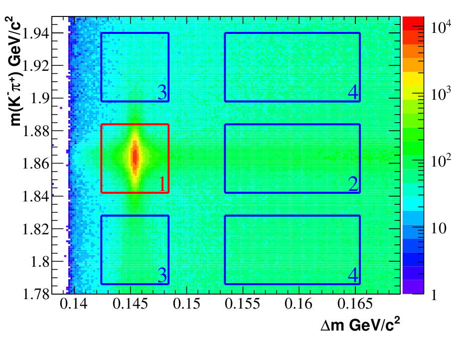
This background subtraction procedure has been carried out for the distribution for each bin of using the following steps:
- 1.
consider the no PID sample in the m() sideband regions; divide the number of events in the signal region by the number of events in the sideband to get the scale factor to go from sideband to signal in ;
- 2.
in the good PID sample scale the m() spectrum in the sideband region using the factor obtained in the previous step; then integrate the resulting m() spectrum to get the factor to rescale background;
- 3.
use the factor measured in step 2 to rescale the interesting distribution () obtained from the events of the no PID sample in signal, m() sideband region (category 4);
- 4.
subtract the distribution obtained in step 3 from the same distribution retrieved from good PID sample in signal region.
This procedure has been carried out for the distribution for each bin of . All the histograms have been then fit to the convolution of Eqs. 21 and 23 to determine the parameters of the efficiency function and . Measuring and for data and MC, we can evaluate the systematic error using Eq. 24. The fit makes use of a global defined as
| (25) |
where is the index referring to one of the 8 regions, refers to one of the 16 bins of the histogram in that region. , and are the number of events observed in the bin, its error and the number of events expect by the fit model, respectively. The expression of the fit model is
| (26) |
where indicates the bin of the distribution in the region, and is one of the 10 bins of the detailed distribution within the range of momentum considered in the region.
The number of floating parameters in the fit are 18: 8 normalization factors , 8 (one for each bin) from Eq. 21, and and from Eq. 23. The fit has been made both to data and MC, giving the results shown in Fig. 23 and Tab. 2.


| Parameter | MC | Data |
|---|---|---|

Finally, the efficiency functions are compared in Fig. 25. Please note that these distributions include acceptance. The method shown herein does not allow to disentangle the acceptance from the soft pion efficiency. The systematic uncertainty estimated from Eq. 24 for the low tracks is .

8 reconstruction efficiency measurement
A significant number of analyses in BABAR involve the reconstruction of the decay , where the two charged pions belong to the list CT of all reconstructed tracks in the event. The track reconstruction efficiency for charged tracks originating within 15 mm in XY from the beam spot is studied by the other methods presented earlier in the paper. However, most of the ’s decay outside this 15 mm radius, making it necessary to understand the daughter reconstruction efficiency in data and MC.
The reconstruction efficiency of the daughters depends on the transverse momentum, , polar angle, and transverse () flight distance, , which is computed as the distance between the primary vertex of the event and the refitted decay vertex.
The general strategy is to subdivide the data and MC events into a large number of samples by choosing an appropriate binning in these variables, determine the number of ’s in each bin in data and MC and, for each of the momentum and polar angle ranges, normalize the ratio of its value in the first bin in , where all tracking effects are understood to 1.000 by definition, with no associated error other than the systematic uncertainty per track, as discussed in Section 4. Bin sizes are optimized to ensure a sufficient number of events in each bin, with 4 bins in (0.0 - 0.4 - 1.0 - 2.0 - 4.0 GeV/c), 8 bins in () and 10 bins in (0.0 - 0.3 - 1.3 - 2.78 - 3.2 - 4.0 - 5.4 - 9.1 - 11.4 - 23.6 - 40.0 cm). The binning in roughly reflects the structure of the BABAR detector and the bins are numbered from 0 to 9, bin 1 being the normalization bin. The normalized ratio of the data and MC as a function of different bins is provided as a correction factor for the daughter reconstruction efficiency. In order to reduce the uncertainty from the imperfect simulation of the random track background or the potential differences between the quality cut efficiencies in data and MC, we remove the immediate vicinity of the event’s primary vertex which is 3 mm in XY from the first (normalization) bin.
Events of interest are selected by looking for the (with ) decays in the data and MC samples. The MC sample includes events from generic B decays, light quark events (u,d,s,c) and decays. The is reconstructed from two oppositely charged tracks, the invariant mass of which is required to be within 25 MeV/ of the PDG value of the mass ( = 497.614 0.024 MeV/) [6]. The two oppositely charged tracks must originate from a common vertex and the fit is required not to fail. The event is required to have at least five GT tracks, two of which are oppositely charged GT tracks that when combined with the candidate to form an object with GeV/ and GeV. About 93% of these events come from the light quark (udsc) continuum; the contribution from production is about 2.5% and only about 3.5% of candidates arise from B decays, most of which are random track combinations. Figures 26 and 27 show the data and MC comparison of the mass, , and distributions for the reconstructed candidates.


To determine the number of ’s in each of the bins in data and MC, the mass distributions in each of the bins are fitted with a sum of a double Gaussian and a constant background. The constant background, determined from the sideband regions in the mass distribution, [0.476, 0.485] U [0.511, 0.520] GeV/, for each bin, is then subtracted to determine the number of in each bin. The limited statistics in a large fraction of bins makes it impractical to allow the slope of the background to float. The binned maximum log likelihood method is used since the default -minimization method is less appropriate in this study as it systematically, in a statistics-dependent way, underestimates the number of events in each bin.
We define the values of the normalized ratios and the uncertainties , where the indices , and stand for the number of the , and bins respectively, to be
| (27) |
| (28) |
where and are the numbers of ’s and their uncertainties in data and and are the numbers of ’s and their uncertainties in MC. We also take into account the difference in the mass resolutions in data and MC by performing numerical integration to determine the efficiencies of the MeV/ cut in data and MC. The efficiency corrected normalized ratio, , also called the correction factor, is computed for each bin and also as a function of several different sets of quality cuts (cuts on the mass, 3-D or flight length or its significance, the 3-D or angle, between the momentum and the line connecting the decay vertex and the primary vertex of the event, and, in one instance, a cut on the vertexing quality), which also enables us to study the systematic uncertainties associated with a correction factor.
To get the overall correction in the daughter reconstruction efficiency in an analysis, we apply the correction factors to the signal MC. If is the number of events in the signal MC sample that falls within the bin (ijk), the relative weight of a reconstruction efficiency correction table element is / , where = and its statistical uncertainty is . The central value of the overall data/MC efficiency ratio is simply given by
| (29) |
Calculation of the statistical uncertainty on this number is slightly non-trivial since we have to take into account the fact that the statistical uncertainty on the normalization bin ratio, , influences the entire row (ij). Substituting in Eq. 29 with the expression in Eq. 27 and differentiating the resulting expression with respect to each of the variables that enter it while using = 1, we obtain
| (30) |
where the first term reflects the finite size of the signal MC sample used in the study and is generally the smallest, the second term reflects the statistical uncertainties on the number of ’s in bins other than the normalization bin, and the third term, the dominant one, reflects the dependence on the statistical precision of of the correction factors in each of the bins , .
The correction factors are applied to signal MC for the decay modes and , which provide spectra representative of most cases of used in BABAR analyses, to determine the overall correction factor and its statistical error. The above exercise is repeated for several sets of quality cuts, from none to tight, and for three different binning approaches. Half of the largest deviation in the correction factors for different quality cuts is considered to be the systematic uncertainty associated with daughter reconstruction efficiency. For these modes we are able to determine the ratio of the data and MC daughter reconstruction efficiency to be about 99.5% and with a statistical error of and a systematic uncertainty of 0.7%.
9 Conclusion
In conclusion, we studied the track reconstruction efficiency of charged particles in BABAR over a wide range of momentum, polar angle, and track separation. Our results come from several different control samples, which are observed to be self-consistent, and well modeled in MC. The overall reconstruction efficiency for isolated tracks is found to be consistent with MC predictions. We also measured the charge asymmetry in the track reconstruction, which was found be consistent with zero. Any observed difference between data and MC in the track reconstruction efficiency could be considered as a source of systematic uncertainty in all the physics analyses in BABAR. For physics analyses with low multiplicity and similar topology to the Tau31 decays and for charged tracks with momentum greater than 180 MeV/c, the results from the Tau31 study should be used; for other B and D decays, the results from the ISR study could be considered. For charged tracks with momenta less than 180 MeV/c, an additional systematic uncertainty of 1.54% per track should be applied. The reconstruction efficiency in data and MC is found to be a function of momentum, polar angle and transverse flight distance, which needs to be considered for reconstruction in BABAR.
10 Acknowledgements
We are grateful for the extraordinary contributions of our PEP-II colleagues in achieving the excellent luminosity and machine conditions that have made this work possible. The success of this project also relies critically on the expertise and dedication of the computing organizations that support BABAR. The collaborating institutions wish to thank SLAC for its support and the kind hospitality extended to them. This work is supported by the US Department of Energy and National Science Foundation, the Natural Sciences and Engineering Research Council (Canada), the Commissariat à l’Energie Atomique and Institut National de Physique Nucléaire et de Physique des Particules (France), the Bundesministerium für Bildung und Forschung and Deutsche Forschungsgemeinschaft (Germany), the Istituto Nazionale di Fisica Nucleare (Italy), the Foundation for Fundamental Research on Matter (The Netherlands), the Research Council of Norway, the Ministry of Education and Science of the Russian Federation, Ministerio de Ciencia e Innovación (Spain), and the Science and Technology Facilities Council (United Kingdom). Individuals have received support from the Marie-Curie IEF program (European Union), the A. P. Sloan Foundation (USA) and the Binational Science Foundation (USA-Israel).
References
- [1] J. Sulkimo et al., Nucl. Inst. and Meth. A 506 250 (2003), J. Allison et al., IEEE Trans. Nucl. Sci. 53 270 (2006).
- [2] P. Golonka et al., Comput. Phys. Commun. 174 818 (2006), P. Golonka and Z. Was, Eur. Phys. J. C 45 97 (2006).
- [3] D. J. Lange, Nucl. Instr. Methods Phys. Res., Sect. A 462, 152 (2001).
- [4] B. Aubert et al. (BABAR Collaboration), Nucl. Instr. and Methods A 479, 1 (2002).
- [5] D. Brown, talk presented at CHEP97, http://www.ifh.de/CHEP97/abstract/a341.htm.
- [6] K. Nakamura et al. (Particle Data Group), J. Phys. G 37, 075021 (2010).
- [7] B. F. Ward, S. Jadach, and Z. Was, Nucl. Phys. Proc. Suppl. 116, 73 (2003).
- [8] S. Jadach, Z. Was, R. Decker, and J. H. Kühn, Comp. Phys. Comm. 76, 361 (1993).
- [9] E. Barberio and Z. Was, Comp. Phys. Comm. 79, 291 (1994).
- [10] T. Sjostrand, Comput. Phys. Commun. 82, 74 (1994).
- [11] S. Jadach and Z. Was, Comput. Phys. Commun. 85, 453 (1995).
- [12] V.P.Druzhinin, http://www.slac.stanford.edu/BFROOT/www/Physics/Tools/generators/AfkQed.ps.
- [13] H. Czyż, J.H. Kühn,A. Grzelinska and J.H. Kühn, Phys. Rev. D 81, 094014 (2010).
- [14] B. Aubert et al. (BABAR Collaboration), Phys. Rev. D 70, 072004 (2004).
- [15] B. Aubert et al. (BABAR Collaboration), Phys. Rev. D 73, 052003 (2006).
- [16] B. Aubert et al. (BABAR Collaboration), Phys. Rev. D 76, 092005 (2007).
- [17] B. Aubert et al. (BABAR Collaboration), Phys. Rev. D 76, 012008 (2007).
- [18] B. Aubert et al. (BABAR Collaboration), Phys. Rev. D 77, 092002 (2008).
- [19] B. Aubert et al. (BABAR Collaboration), Phys. Rev. D 78, 011105 (2008).
- [20] S. Menary, CLEO Internal Note, CBX 92-103 (1992) (unpublished).
- [21] G. Brandenburg et al. (CLEO Collaboration), Phys. Rev. D 58, 052003 (1998)
- [22] L. Gibbons et al. (CLEO Collaboration), Phys. Rev. D 56, 3783 (1997)
- [23] Charge-conjugate reactions are implied throughout this paper except for section 6.