Model of joint displacement using sigmoid function. Experimental approach for planar pointing task and squat jump
Abstract.
Using an experimental optimization approach, this study investigated whether two human movements, pointing tasks and squat-jumps, could be modelled with a reduced set of kinematic parameters. Three sigmoid models were proposed to model the evolution of joint angles. The models parameters were optimized to fit the 2D position of the joints obtained from 304 pointing tasks and 120 squat-jumps. The models were accurate for both movements. This study provides a new framework to model planar movements with a small number of meaningful kinematic parameters, allowing a continuous description of both kinematics and kinetics. Further researches should investigate the implication of the control parameters in relation to motor control and validate this approach for three dimensional movements.
Key words and phrases:
Sigmoid, Optimization, Predicted model, Pointing task, Squat jump.1. Introduction
Quantitative analysis of human movement usually relies on the time history of reflective markers fixed to anatomical landmarks obtained from optical systems. These raw data are further used to compute relevant parameters such as velocities, accelerations, moments or powers. During the recent years, the performance of acquisition systems greatly increased, especially consdiering acquisition rate and accuracy. However, raw data still remain noisy, due to the movement of the skin with regard to the bones and finite accuracy of such systems. Furthermore, the effect of noise increases as the data is derived with respect to time, which is a very common task in movement analysis.
To overcome the aforementionned issues, raw data are quite always smoothed or filtered, resulting in well-known decrease of movement amplitude. Specific filtering methods accounting for properties of the skeletal system such as constant length of the limbs have been used but such approaches still suffer from the motion of the markers relatively to the skeletal system. An interesting feature of human motion is the necessity for decelerating the joint displacement before its maximal amplitude (anatomical constraint) in order to protect this joint from any damage [IS89]. Regarding to kinematics, the anatomical constraint implies that joint angular time history should match an asymmetric sigmoid shape [ZSG86] and thus an asymmetric bell-shaped velocity profile [SL81], which accounts for synergistic actuators’ activations at a joint, i.e. agonist and antagonist muscle-tendon systems. In the field of human movement analysis, Plamondon proposed an asymetric model of asymetric sigmoid [Pla95a, Pla95b, Pla98, PCF03] but the velocity is not null at the end of the movement so that the anatomical constraint is not satisfied.
Therefore, this study aimed at modelling two different movements, i.e. a pointing task and an explosive movement, the squat-jump, using a generic model of sigmoidal joint displacement based on meaningfull kinematic parameters which accounts for the anatomical constraint. Three submodels were used to achieve best fitting of experimental data obtained from both movements.
2. Methods
2.1. Model of joint displacement
2.1.1. General model
Accounting for a monotone evolution of a given angle and considering the anatomical constraint requirements, it is assumed that each angle is characterized by the following properties (figure 1):
- —
at the beginning and at the end of the movement, the velocity and the acceleration are equal to zero;
- —
the angle increases (respectively decreases) throughout the whole movement;
- —
during the movement, the velocity increases (respectively decreases) until it reaches its maximum (respectively minimum), then decreases (respectively increases).

More precisely, we try to determine a function from to of class . Let be three instants such that
| (2.1) |
Let be three real numbers such that
| (2.2) |
We assume that
- —
is constant and equals on ;
- —
is constant and equals on ;
- —
there exists such that is strictly increasing on ;
- —
is strictly convex on ;
- —
is strictly concave on .
We set
| (2.3) | ||||
| Let be the number defined by | ||||
| (2.4) | ||||
Since is of class , we have
| (2.5a) | ||||
| (2.5b) | ||||
| (2.5c) | ||||
| (2.5d) | ||||
| (2.5e) | ||||
We consider and defined by
| (2.6) |
Applying the following change of scale,
| (2.7a) | ||||
| (2.7b) | ||||
the problem can be reformulated as follows: we look for a function of class defined on satisfying:
| (2.8a) | ||||
| (2.8b) | ||||
| (2.8c) | ||||
| (2.8d) | ||||
| (2.8e) | ||||
Finally, the function is defined for all , by
| (2.10) |
This function is defined by 7 independent parameters:
- —
2 time scale parameters ( and ),
- —
2 angle scale parameters ( and ),
- —
and 3 shape parameters (, , ).
Thus, can be written under the form .
In the literature, there exist many sigmoidal functions. However, these models can not be used to solve (2.8) because the sigmoids
- —
- —
- —
To our knowledge, there is not in the literature, a general construction of non symmetric sigmoid satisfying (2.8), of class or .
In the field of movement analysis, R. Plamondon [Pla95a, Pla95b, Pla98, PCF03] used a log-normal function
| (2.11) |
to describe general movements and applied it to the Fitts task [MF54, MFP64]. By using the Central Limit Theorem, he proved that, for a large number of agonist and antagonist muscles acting, the proposed function can model the behavior of the system. However, this work can not be applied to solve (2.8). The major concern with Plamondon’s function remains in its asymptotic behavior at the end of the movement. Especially, it should be observed that the velocity tends to zero as approaches and then, the end of movement is not clearly defined. Other works related to the log-normal law [LG63, Bra70, Pea91] do not solve this problem. Moreover, Plamandon’s model contains not enough parameters to allow the solving of (2.8).
The simplest idea to solve (2.8) would be to apply Hermite’s polynomial interpolation (e.g. [CdB81]), but it can be showed that this method can not be used (see [BC13]).
To allow the solving of the system (2.8), the model has to include three control parameters which have to be determined in relation to , and . In the next section, three sigmoid models, SYM, NORM and INVEXP, previously described in [Cre09], meeting the mentioned requirements are presented. These models were successfully used for both pointing tasks [Vil08, VBML08, LCB11] and squat-jump [Cre09, CBL09]. Exhaustive theoretical description of the models will be given in a future paper [BC13].
2.1.2. The SYM model
The SYM model was built using a pseudo-symmetry approach. Its function is defined by the three parameters and .
Let be a function of class from to satisfying (2.8a),(2.8c), and (2.8d). If the function is defined from to by,
| (2.12) |
then, is of class on and (2.8) holds. Considering the function defined on for all and by
| (2.13) |
, and have to be determined so that (2.8a), (2.8c) and (2.8d) hold. We set
| (2.14) |
For all , for all such that , there exist such that (2.8a), (2.8c) and (2.8d) hold for function . , and still need to be defined. We set
| (2.15a) | |||
| It exists a unique such that | |||
| (2.15b) | |||
| and it follows | |||
| (2.15c) | |||
By setting , the function is defined for all by
| (2.16) |
2.1.3. The NORM model
The NORM model (named from its relation to the normal law) function is defined by three parameters , and .
We recall that the density function of the the normal (or Gaussian) distribution with mean and variance is given by:
| (2.17) |
Considering the function defined by
| (2.18) |
the cumulative distribution function of the normal law is given by
| (2.19) |
For all , we define the bijection from to by
| (2.20) |
Finally, the function is defined by
| (2.21a) | ||||
| (2.21b) | ||||
| (2.21c) | ||||
with .
2.1.4. The INVEXP model
The INVEXP model (derived from the inverse exponential) function is defined by three parameters and . For all , for all , we set
| (2.22) |
and we consider function defined by if
| (2.23a) | ||||
| and if | ||||
| (2.23b) | ||||
For all and for all , we consider the function defined by
| (2.24) |
For all , is defined by
| (2.25a) | ||||
| (2.25b) | ||||
| (2.25c) | ||||
For all , is defined by
| (2.26) |
and finally the function is defined by
| (2.27) |
2.1.5. Definition domains of the sigmoid models
Each of the three functions is defined by three parameters. We will prove in [BC13] that for all , there exist a part of such that for all , there exist at least one sigmoid of kind satisfying (2.8) whose parameters can be determined by splitting (2.8) in three non-linear equations which can be solved with a numerical solver. This part is different for the three sigmoid models. The bigger part is obtained with the INVEXP model and is given by
| (2.28) |
This domain is a polygonal part of . The domain of a function satisfying (2.8) can not be bigger thanks to (2.9). The domain of SYM sigmoid, which is also a polygonal part of is given by
| (2.29) |
where is defined by (2.14). The domain of NORM sigmoid can be determined numerically. It should be noticed that these three domains are symmetric according to the point and this point belongs to the three domains (Fig 2).


Examples of position and velocity curves obtained from the three models are provided in figure 3. Each sigmoid is defined by , belonging to a fixed straight line and .
2.1.6. Specific properties of the sigmoid models
- —
The model SYM is very simple and fast to calculate; however, the class of this model is only versus for the two other models.
- —
Since the function is directly implemented in most numerical softwares, the model NORM is fast to calculate. However, the domain of this model has been obtained by symmetrization, and for some values of , two different sigmoids can be obtained. Moreover, the determination of the definition domain is not trivial and the function does not meet the concavity and convexity requirements outside of it.
- —
The part of model INVEXP is the biggest, but this model is harder to calculate, because a numerical method of integration has to be used. Since efficient numerical methods exist, this problem can be overcomed and computation time remains reasonable.
2.2. Experimental procedures


2.2.1. Pointing task
9 right-handed male subjects (age: , height: cm and mass: kg) were asked to perform pointing tasks in the horizontal plane. The total number of pointing tasks was 304. Movements were performed for five directions and two distances (Fig 4). For each direction, two spherical targets were placed on a table at 60 and 80 cm from the shoulder. Directions of pointing task ranged regularly from to including pointing along the antero-posterior axis. The described position of the targets ensures that each of them is located inside the subjects workspace (Fig 5) when considering a 80 cm upper limb length and anthropometric data presented in [BLM10]. At the beginning of the movement, subjects had to position their arm so that the forefinger is located at 40 cm of the soulder in the antero-posterior direction. During the experiment, subjects sat on a chair whose height was adjusted so that the upper limb remained in the horizontal plane while moving over the table from starting point to targets and the trunk was immobilized by using straps. In order to ensure that the upper limb remained in the horizontal plane, the subjects were instructed to keep the upper limb lying on the table during the movements. Video reflective markers were placed on the subjects at the shoulder (acromion), elbow (olecrane), wrist (middle of radial and ulnar styloid processes) and forefinger extremity to allow further modeling of the upper limb. For each target, subjects performed three movements which were filmed at 25 Hz with a numeric camera JVC ©Everio placed above the subjects and oriented vertically. Raw experimental data, i.e. the position of the joints throughout the movement, were extracted from videographic recordings.
2.2.2. Squat jump
The squat-jump data was obtained from a previous work [BBM12]. Each of 13 other subjects performed 10 vertical jumps. Instructions were given for keeping the hands on the hips during the movement to limit the contribution of the upper limbs to the performance. Furthermore, subjects were asked to do no countermovement. The jumps which did not meet both of these requirements were excluded from the study. In order to model the skeleton in a 4 rigid segments system, landmarks were placed on the left fifth metatarsophalangeal, lateral malleolus, lateral femoral epicondyle, greater trochanter and acromion. These landmarks define the foot, the shank, the thigh and the upper body (Head, Arms and Trunk: HAT). The subjects were filmed orthogonally to the sagittal plane at 100 Hz and the ground reaction force was recorded at 1000 Hz from an OR6-7-2000 AMTI force plate. The center of mass (CoM) position of limbs was computed using anthropometric data [Win90]. The whole body CoM (Center of Mass) position was determined on the one hand from kinematic data and on the other hand from force plate measurements using a double numerical integration procedure. For the latter, subject mass, initial body CoM position and velocity had to be set. These values were computed so that the difference between CoM path obtained from kinetic and kinematic data was minimized in a least square sense. This optimization step was also used to synchronize both recording sources.
2.3. Skeletal model

For both tasks, the studied limbs were modeled as rigid bodies rotating around frictionless hinge joints. Given limbs, the joint positions are defined by the points () with and for pointing task and squat-jump respectively. From this definition, the position of the joints in the direct orthonormal reference frame are related in the complex sense to limb lengths and angles (Fig 6) and the affix of is given by
| (2.30) |
for all , where is the imaginary unit and is the affix of .
It should be noticed that and are segmental and joint angles respectively (Figure 6). According to these definitions, the velocities and other derivatives of the joint positions with respect to time can be computed from corresponding derivatives of and .
Remark 2.2.
The determination of the positions, velocities and accelerations of the points require that the coordinates and further derivatives of are known. Three cases should be considered to calculate and :
- —
the point is fixed;
- —
the point belongs to a simple curve such as a circle or a parabola;
- —
the center of mass of the subject and angle , are known.
2.4. Movement model
Considering limbs as rigid bodies, the relative positions of joints are directly related to the angles according to (2.30).
The evolution of the angles throughout the movement was modeled using three types of sigmoid shaped curves. The parameters of the sigmoids were computed using an optimization procedure so that the experimental and modeled markers trajectories are closest from each other in the least square sense. Theoretical results of this section have been already partially given in [Cre09] and will be presented extensively in a future work [BC13]. We recall that to allow dynamic continuity, the required solutions should be models of class at least, defined on and satisfying (2.8).
2.5. Data processing
Experimental pointing task and jumping data were modeled using the sigmoid models. Specific procedures are described below.
2.5.1. Shoulder path

Experimental data obtained from pointing tasks show that the shoulder joint path is well fitted by an arc of circle for all subjects (Fig. 7). This movement was observed in spite of trunk immobilization. Since shoulder is a patella type articulation, this result is not surprising. The characteristics of the circle can be determined using a least squares method. The center and radius of the circle minimizing the distance sum of squares between experimental data and theoretical data were researched. Firstly, a direct method was used to minimize the sum of
Secondly, the sum
was minimized by using an iterative method. For this method, the results of the direct optimization were used as initial values for and . This final optimization was performed with the library Matlab least squares geometric element software, available at http://www.eurometros.org/gen_report.php?category=distributions&pkey=14. For more details, see [Raz97, Raz98, ARW01, EMM07, MK91, Fan90, CJ89].
We set , and we consider then angle defined by:
| (2.31) |
We assume then that and are constant and we obtain
| (2.32) |
where , and are known. We add then Eq. (2.30); thus, assumption of remark 2.2 holds.
The mechanical system is plotted on Fig. 6; the coordinates of and the lengths , , and are constant and the experimental data are then angle , , and .
2.5.2. Determination of sigmoid parameters
Sigmoid parameters were obtained from a multi-stage optimization procedure. First, and were estimated from experimental data. The scale parameters were defined so that the absolute peak angle velocity occurs between and and the angle velocity sign changes at the endpoints of this interval. Considering and as the angle values at and , the shape parameters and were determined thanks to Eq. (2.6).
First optimization consisted in minimizing the sum of square of differences between experimental angles and those obtained from the sigmoid models for each of instants:
The optimization was achieved for each sigmoid with the lsqcurvefit function provided in Matlab software. Initial values of parameters were set from estimations of experimental data described previously. This optimization stage will be further referred to as local optimization.
Secondly, differences between experimental and model reconstructed joint positions were minimized in a least square sense. The objective can thus be written as
Compared to the previous stage, this optimization can be considered as global since for the latter, the parameters of the sigmoids were determined simultaneously. Computation of model-based joint positions implies the lengths of the limbs to be provided. For the pointing tasks, the optimization was performed using (i) mean experimental limb lengths (semi-global optimization) and (ii) limb lengths as model parameters (global optimization).
2.5.3. Squat-jump specific procedure
The modeling of the jump focused on the position of the joints in a reference frame located at the distal extremity of the foot. Thus, the optimization consisted in fitting the experimental joint positions of ankle, knee, hip and shoulder with the model parameters in this reference frame. Since joints do not remain fully extended after the take-off, differences were not taken into account during the whole movement. This prevented the model from underestimating the necessary amplitude of joint extensions. Therefore, differences between experimental and model-based data were considered during the intervals corresponding to increase of vertical joint coordinates in the given reference frame (e.g. the error at the ankle joint was only taken into account while the vertical distance between the knee and the foot extremity increased). The objective was used to achieve this optimization stage, which will be further related as kinematic.
Second stage of optimization included non-linear constraints on position, velocity and acceleration of the body CoM computed from sigmoid model. It was imposed that the body CoM position computed from both the sigmoid model and the force plate data were similar at the instant for which the marker located on the distal extremity of the foot started to move upward. At this instant, equality for the coordinates of both velocity and acceleration of body CoM obtained from kinetic and kinematic data was also required. Finally, body CoM vertical acceleration was constrained to be greater than -9.81 m.s-2 before ensuring that take-off occurs necessarily after . From to the end of the jump, the movement of was set so that kinetic and kinematic-based movement of the CoM were similar. This results in a continuous characterization of the movement position, velocity and acceleration. It should be noticed that using similar constraints for jerk and further derivatives could have led to description of class and higher.
2.6. Modeling accuracy
For each instant and joint , the optimization accuracy can be quantified by the difference between experimental data ( and ) and sigmoid modeled data ( and ):
| (2.33a) | ||||
| In further analysis, maximal and mean values of these differences are used to account for the fitting accuracy of the modeling procedures: | ||||
| (2.33b) | ||||
| (2.33c) | ||||
2.7. Statistical analysis
For both maximal and mean errors given in (2.33b) and (2.33c), the Shapiro-Wilk test reported unnormal distributions.
Thus, statistical tests were realized on normally distributed of observations (i.e., errors and computation time).
Firstly, anovas for repeated measures were performed for errors and computation time.
When anovas reported significant results, post-hoc tests were performed to check for differences between the sigmoid models and the optimization procedures.
All the tests were realized with ![[Uncaptioned image]](1207.2627v3/Rlogo.png) [R D11] and statistical significance was set at confidence level, i.e. .
[R D11] and statistical significance was set at confidence level, i.e. .
3. Results
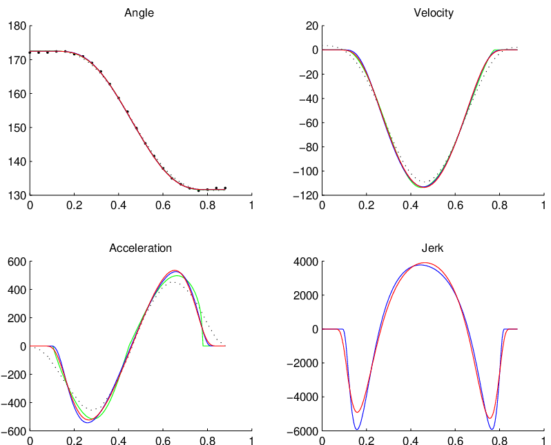
The results obtained from the 304 pointing tasks and 120 squat-jumps are summarized in the tables 2 and 3 for pointing task and 4 and 5 for squat Jumps given in the appendix A. Examples of experimental and modeled data are provided for the pointing tasks and squat-jumps in the figures 8 to 11 and 14 to 17 respectively. Plots of velocities, accelerations and jerks of modeled data were obtained from analytical derivation of sigmoid models with respect to time.
The obtained results are very accurate from numerical viewpoint. Indeed, for pointing task, in 95% of cases, for the three models, the maximal error (defined by (2.33b), i.e. the difference between the calculated trajectories and the experimental trajectories for local method and is smaller than
| (3.1a) | ||||
| and for semi-gobal or global error, and it is smaller than | ||||
| (3.1b) | ||||
| The mean error (defined by (2.33c)) for the three methods is smaller than | ||||
| (3.1c) | ||||
For for squat jumps, the maximal error for the best method, i.e. the kinematic one is smaller than
| (3.2a) | ||||
| and the mean error for the kinematic method is smaller than | ||||
| (3.2b) | ||||




3.1. Pointing task
Recall that for
- —
’***’ means ;
- —
’**’ means ;
- —
’*’ means ;
- —
’.’ means .
Among the three anovas performed for computation time, maximal and mean errors, the highest p-value was equal to (***) suggesting that both optimization methods and sigmoid models are associated to significantly different results.
Considering both mean and maximal errors, post-hoc tests revealed greater adequation of original data with semi-global optimization procedure than with local one () for each of the three sigmoid models.
Computation time reported for semi-global optimization was significantly higher than durations obtained with local method for SYM and INVEXP models () but not for NORM one ().
Comparing semi-global and global methods revealed no significant difference for computation time (), maximal ( 0.3291) and mean ( 0.6166) errors.
For the local optimization case, no significant difference was found between the three sigmoid models when comparing maximal () and mean () errors. Similar results are obtained for global (maximal: , mean: ) and semi-global (maximal: , mean: ) cases.
3.2. Squat Jump
Basic descriptive statistics of measured values are given in tables 4 and 5. Examples of experimental and modeled joint angles time histories are presented for both kinematic and dynamic optimization methods in the figures 14 and 15 respectively. Time histories of relative joints position are presented in the figure 16.
Among the three anovas performed for computation time, maximal and mean errors, the highest p-value was equal to (***) suggesting that both optimization methods and sigmoid models are associated to significantly different results.
Compared to constrained optimization, unconstrained method executed faster () and fitted better kinetic original data for both maximal and mean errors () whatever the sigmoid model.
Considering the unconstrained optimization, no significant difference was found between the sigmoid models for maximal () and mean () errors.
Post-hoc tests revealed significant differences between the sigmoid models for the constrained optimization method. Maximal errors mesaured for NORM model were higher than those obtained from SYM ( (***)) and INVEXP ( (*)). Considering mean errors, SYM model fitted best the original data compared to NORM ( (***)) and INVEXP ( (***)).
4. Discussion
This study evaluated different optimization methods to fit joint trajectories produced during pointing tasks and squat jumps. The evolution of joint angles during the movements was modeled using three sigmoid shaped functions. Assuming a constant length of the limbs, the whole movement was reconstructed from the sigmoid models parameters. For each movement type (i.e. pointing tasks and squat jumps) and sigmoid model, different optimization methods were investigated.
In the literature, only Plamondon used a similar approach. However among the published articles, experimental data were presented only in [Pla98]. Furthermore, no quantitative results were provided and the data was presented for a single subject. This does not allow to compare the present models with Plamondon’s one. However, as mentioned earlier, the models used in the present study are defined on a bounded time interval contrarily to the log-normal models for which the end of the movement is not clearly defined.
4.1. Rigid bodies assumption
Differences between original and reconstructed data were lower for pointing tasks than for squat-jumps. This result could be explained by the relatively greater amplitude of the joint trajectories during the jumping movement. Moreover, the modeling of the skeleton assumes rigid bodies between the joints. Considering the pointing tasks, it can be supposed that the length of the modeled limbs is quite constant. This assumption is supported by the similarity of the errors observed for global and semi-global methods. The rigid bodies assumption would be less true for squat-jump, especially for the trunk limb. Indeed, the spine is composed of many joints which allow bending of the trunk and thus, the trunk may be divided into two [KdLT+96, dLKBT92, PGD96] or three [dL93] segments to ensure that the rigid bodies model is close enough to the reality of the movement.
4.2. Planar movement
The modeling methods proposed in this study deal with planar movements. The higher errors obtained with modeling of squat jumps may be explained by the movement of the joints along the transverse axis, especially for the knee. In comparison, pointing tasks would be closer to a real planar movement since the movement is performed on a planar surface.
4.3. Optimization methods computing velocity
Considering the pointing tasks, computation lasted longer for semi-global method than for local one. Global optimization executed with similar velocity compared to semi-global method. Thus, global optimization should be used unless specific purposes are researched. For the squat-jumps, the present results show that unsurprisingly, using the constrained method is much more longer than the unconstrained optimization.
4.4. Optimization methods accuracy
For pointing tasks, accuracy of the model was higher for semi-global optimization than for local one. This suggest that modeling should consider the joints movements together to achieve better fitting of original data. It should be noticed that local optimization could have considered the dependence of the distal joints trajectories to the proximal ones. Global optimization did not lead to better results compared to semi-global method. This result is consistent with both the planarity of movement and rigid bodies assumptions.
4.5. Sigmoid models accuracy
| SYM | NORM | INVEXP | |
| Computation time | + | +++ | + |
| Definition space | ++ | + | +++ |
| Accuracy | 0 | 0 | 0 |
| Mathematical regularity | + | +++ | +++ |
For both pointing tasks and squat jumps, similar accuracy was obtained with the three models of sigmoids. Among the two movements and the optimization methods, it appears that the NORM model allows fastest computation. Considering SYM and INVEXP models, their relatively slower execution can be explained by the non-linear equation solving and the numerical integration respectively. NORM model formulation takes advantage of the native implementation of the erf function in Matlab software thus ensuring fast computation.
4.6. Practical considerations
The present results show that joint trajectories during planar movements such as pointing tasks or squat-jumps can be modeled using meaningful kinematic parameters. Table 1 presents a summary of the results obtained with the different optimization methods and sigmoid models.
Among the three sigmoid models tested in this study, it appears that the NORM model is computed faster and allows better data fitting of the pointing tasks than other models. On the contrary, for squat-jumps, INVEXP and SYM models fitted better original data. From these results, it can be suggested that INVEXP and NORM models should be used preferentially. Indeed, the INVEXP model did not lead to better results and needs substantial computation time compared to other models. Despite the important computation time, INVEXP model may be useful for modeling specific movements, especially fast movements, which may not allow a good fitting with NORM model due to the relatively small definition domain of this model in the space. For relatively slow and smooth movements, NORM model should be primarily used.
Considering the class of the three models, INVEXP or NORM models should be used when the jerk has to be computed, since it can be analytically determined from the models formulation. If the jerk is not considered as a relevant parameter, both velocities and accelerations can be obtained analytically whatever the used model. Furthermore, slow data acquisition rates should not affect much the quality of the fits since only three points are needed to compute the shape parameters of the three models.
5. Conclusion
This study shows that complex planar movements can be modeled by using a small set of meaningful kinematic parameters defining the time history of joint angles with high accuracy (in 95% of cases, mean errors obtained from pointing task and squat jump were respectively inferior to 1 and 3 centimeters). This approach can provide a continuous description of the movement and thus may be used to analyze the evolution throughout the movement of parameters which need differentiation of raw data with respect to time without performing numerical computations. Especially, this could avoid well known magnification of error resulting from such procedure. Furthermore, the modeling procedure can be applied for fast movements, as well as when acquisition rate is slow, as only 3 points are required to get the sigmoid parameters. Moreover, the flexibility of the new sigmoid models should lead to increased realism of movements obtained from procedural animation. Further researches should assess the relevance of such modeling strategy for three dimensional movements and the relation between the model parameters and the central nervous system processes implied in motor control.
Appendix A Set of tables of statistical results
A.1. Pointing task
| data | method model | SYM | NORM | INVEXP |
|---|---|---|---|---|
| computation time | local | |||
| semi-global | ||||
| global | ||||
| maximal error | local | |||
| semi-global | ||||
| global | ||||
| mean error | local | |||
| semi-global | ||||
| global |
| data | method model | SYM | NORM | INVEXP |
|---|---|---|---|---|
| maximal error | local | |||
| semi-global | ||||
| global | ||||
| mean error | local | |||
| semi-global | ||||
| global |
A.2. Squat Jumps
| data | method model | SYM | NORM | INVEXP |
|---|---|---|---|---|
| computation time | kinematic | |||
| dynamic | ||||
| maximal error | kinematic | |||
| dynamic | ||||
| mean error | kinematic | |||
| dynamic |
| data | method model | SYM | NORM | INVEXP |
|---|---|---|---|---|
| maximal error | kinematic | |||
| dynamic | ||||
| mean error | kinematic | |||
| dynamic |
References
- [ARW01] Sung Joon Ahn, Wolfgang Rauh, and Hans-Jürgen Warnecke. Least-squares orthogonal distances fitting of circle, sphere, ellipse, hyperbola, and parabola. Pattern Recognition, 34(12):2283–2303, 2001.
- [BBM12] Jérôme Bastien, Yoann Blache, and Karine Monteil. Estimation of anthropometrical and inertial body parameters using double integration of residual torques and forces during squat jump. Submitted to Journal of Biomechanical Engineering. Aivalable on http://utbmjb.chez-alice.fr/recherche/articles_provisoires/squatJump_JBYBKM_2013.pdf, 2012.
- [BC13] J. Bastien and T. Creveaux. Modelling of joint displacement by sigmoid function. Mathematical formalization. In preparation, 2013.
- [BLM10] Jérôme Bastien, Pierre Legreneur, and Karine Monteil. A geometrical alternative to jacobian rank deficiency method for planar workspace characterisation. Mechanism and Machine Theory, 45:335–348, 2010.
- [Bra70] Michael W.B. Bradbury. The effect of rubidium on the distribution and movement of potassium between blood, brain and cerebrospinal fluid in the rabbit. Brain Research, 24(2):311–312, 1970.
- [CBL09] Thomas Creveaux, Jérôme Bastien, and Pierre Legreneur. Model of joint angle displacement: application to vertical jumping. In 13 ième congrès international de l’ACAPS, Approche Pluridisciplinaire de la Motrocité Humaine, pages 49–50, Lyon, October 2009.
- [CdB81] D. Conte and C. de Boor. Elementary numerical analysis. An algorithmic approach. Mc Graw-Hill, 1981.
- [CJ89] Maurice G. Cox and Helen M. Jones. An algorithm for least-squares circle fitting to data with specified uncertainty ellipses. IMA J. Numer. Anal., 9(3):285–298, 1989.
- [Cre09] Thomas Creveaux. Des données expérimentales à la modélisation d’un mouvement dynamique : cas du squat-jump. PhD thesis, Université Claude Bernard Lyon 1, 2009.
- [Deb79] C. Debouche. Présentation coordonnée de différents modèles de croissance. Revue de statistique appliquée, 27(4):5–22, 1979.
- [DG06] József Dombi and Norbert Győrbíró. Addition of sigmoid-shaped fuzzy intervals using the Dombi operator and infinite sum theorems. Fuzzy Sets and Systems, 157(7):952–963, 2006.
- [dL93] P. de Leva. Validity and accuracy of four methods for locating the center of mass of young male and female athletes.deleva1993. In Proceedings of the XIVth Congress of the International Society of Biomechanics, pages 318–319, Paris, France, 1993. Imprimerie Laballery.
- [dLKBT92] M. P. de Looze, I. Kingma, J. B. J. Bussmann, and H. M. Toussaint. Validation of a dynamic linked segment model to calculate joint moments in lifting. Clinical Biomechanics, 7:161–169, 1992.
- [Dra95] John A. Drakopoulos. Sigmoidal theory. Fuzzy Sets and Systems, 76(3):349–363, 1995.
- [EMM07] H. Endo, T. Murahashi, and E. Marui. Accuracy estimation of drilles holes with small diameter and influence of drill parameter on the machining accuracy when drillin in mild steel shett. Machine Tools and manufacture, 47:175–181, 2007.
- [Fan90] De Liang Fan. On formulas for calculating parameters of least square circles. J. Southeast Univ., 20(6):96–101, 1990.
- [Fin52] D. J. Finney. Probit analysis. A statistical treatment of the sigmoid response curve. Cambridge, at the University Press, 2 edition, 1952.
- [IS89] van G.J. Ingen Shenau. From rotation to translation: constraints on multi-joint movements and the unique action of bi-articular muscles. Hum Mov Sc, 8:301–377, 1989.
- [KdLT+96] I. Kingma, M. P. de Looze, H. M. Toussaint, H. G. Klijnsma, and T. B. M. Bruijnen. Validation of a full body 3-d dynamic linked segment model. Human Movement Science, 15:833–860, 1996.
- [KS96] Joe Kilian and Hava T. Siegelmann. The dynamic universality of sigmoidal neural networks. Inform. and Comput., 128(1):48–56, 1996.
- [Kum00] Itsuo Kumazawa. Compact and parametric shape representation by a tree of sigmoid functions for automatic shape modeling. Pattern Recognition Letters, 21(6-7):651–660, 2000.
- [LCB11] Pierre Legreneur, Thomas Creveaux, and Vincent Bels. Control of poly-articular chain trajectory using temporal sequence of its joints displacements. Intelligent Control and Automation, 2(1):38–46, 2011.
- [LG63] J Lindenmann and G.E. Gifford. Studies on vaccinia virus plaque formation and its inhibition by interferon I. Dynamics of plaque formation by vaccinia virus. Virology, 19:283–293, 1963.
- [MF54] Paul M. M. Fitts. The information capacity of the human motor system in controlling the amplitude of movement. Journal of Experimental Psychology, 6:381–391, 1954. (Reprinted in Journal of Experimental Psychology: General, 121(3):262-269, 1992).
- [MFP64] Paul M. M. Fitts and James R. Peterson. Information capacity of discrete motor responses. Journal of Experimental Psychology, 2:103–112, 1964.
- [MK91] L. Moura and R. Kitney. A direct method for least-squares circle fitting. Comput. Phys. Comm., 64(1):57–63, 1991.
- [MMMR96] Anil Menon, Kishan Mehrotra, Chilukuri K. Mohan, and Sanjay Ranka. Characterization of a class of sigmoid functions with applications to neural networks. Neural Networks, 9(5):819–835, 1996.
- [Nar97] Sridhar Narayan. The generalized sigmoid activation function: competitive supervised learning. Inform. Sci., 99(1-2):69–82, 1997.
- [PCF03] R. Plamondon and A.W. Chunhua Feng. A kinematic theory of rapid human movements. Part IV. a formal mathematical proof and new insight. Biol. Cybern., 89:126–138, 2003.
- [Pea91] David E. Pearson. Probability analysis of blended coking coals. International Journal of Coal Geology, 19(1-4):109–119, 1991.
- [PGD96] A. Plamondon, M. Gagnon, and P. Desjardins. Validation of two 3-d segments models to calculate the net reaction forces and moments at the l5/s1 joint in lifting. Clinical Biomechanics, 11:101–110, 1996.
- [Pla95a] R. Plamondon. A kinematic theory of rapid human movements. Part I. Movement representation and generation. Biol. Cybern., 72(4):295–307, 1995.
- [Pla95b] R. Plamondon. A kinematic theory of rapid human movements. Part II. Movement time and control. Biol. Cybern., 72(4):309–320, 1995.
- [Pla98] R. Plamondon. A kinematic theory of rapid human movements. Part III. Kinetic outcomes. Biol. Cybern., 78:133–145, 1998.
- [R D11] R Development Core Team. R: A Language and Environment for Statistical Computing. R Foundation for Statistical Computing, Vienna, Austria, 2011. ISBN 3-900051-07-0.
- [Raz97] A. Razet. Résolution analytique d’un cercle de moindres carrés pour une utilisation en interferométrie. Bulletin du Bureau National de Métrologie, 108:39–48, 4 1997. Bureau National de Métrologie, Conservatoire National des Arts et Métier, 292 rue Saint-Martin, 75141 Paris Cedex 03, France.
- [Raz98] A. Razet. Analytical resolution of least-square applications for the circle in interferometry and radiometry. Metrologia, 35:143–149, 1998.
- [SC03] Yogesh Singh and Pravin Chandra. A class of sigmoidal activation functions for FFANNs. J. Econom. Dynam. Control, 28(1):183–187, 2003.
- [SL81] J.F Soechting and F. Laquantini. Invariant characteristics of a pointing movement in man. J Neurosci, 1:710–720, 1981.
- [VBML08] Clément Villars, Jérôme Bastien, Karine Monteil, and Pierre Legreneur. Kimatic modelisation of joint displacement: validation in human pointing task. In Industrial Simulation Conference (ISC 08), CESH, Lyon, France, June 2008.
- [Vil08] Clément Villars. Les tâches de pointages : approches expérimentale et théorique. Master’s thesis, Université Claude Bernard Lyon 1, 2008.
- [Win90] D. Winter. Biomechanics and motor control of human movement. Wiley-Interscience, 1990.
- [YK03] Beong In Yun and Philsu Kim. A new sigmoidal transformation for weakly singular integrals in the boundary element method. SIAM J. Sci. Comput., 24(4):1203–1217 (electronic), 2003.
- [ZSG86] H. N. Zelaznik, R. A. Schmidt, and S. C. Gielen. Kinematics properties of rapid aimed hand movements. J Mot Behav, 18(4):353–372, 12 1986.