125 GeV Higgs Boson, Enhanced Di-photon Rate,
and
Gauged $U(1)_{\rm PQ}$-Extended MSSM

Both the ATLAS and CMS collaborations have announced the discovery of a $\sim 125$ Higgs boson [1, 2], mainly based on the combination of the di-photon and leptonic $ZZ$ Higgs searches at the $\sqrt{s}=7$ and 8 TeV LHC.

This achievement fixes the last renormalizable parameter in the Standard Model (SM). At the same time, it carries important implications for new physics, particularly for low-energy supersymemmtry (SUSY). In the Minimal Supersymmetric Standard Model (MSSM), a SM-like Higgs boson with 125 GeV mass requires large corrections beyond the tree level prediction $(m_{h})_{\rm tr}\approx m_{Z}\cos 2\beta$. Although such an 125 GeV SM-like Higgs boson can be accommodated, careful choices of parameters must be made [3, 4, 5, 6, 7, 8, 9, 10, 11]. Therefore, it is well motivated to consider possible extensions of the MSSM which give additional contribution to the mass of the SM-like Higgs boson at tree level [11, 12, 13, 14].

In this paper, we consider the possibility of enlarging the MSSM gauge symmetry by an additional $U(1)$. Such a gauge symmetry is quite generic in UV completions low energy supersymmetry, and many possible candidates have been proposed (for a review, e.g., see [15]). If its D-term is non-decoupling, it can provides non-trivial contribution to the tree-level mass of the SM-like Higgs boson [16]. In order to get a sizable correction, the Higgs field must be charged under this $U(1)$ symmetry. Moreover, the symmetry breaking scale of this extra U(1) symmetry cannot be much higher than the EW (EW) one.

We will focus on a gauged Peccei-Quinn (PQ) symmetry ($U(1)_{\rm PQ}$), under which by definition the Higgs fields carries non-trivial charges [17]. This can be connected to a possible solution of the $\mu$-problem [18, 19], which is one of the central pieces of using low energy supersymmetry to address the hierarchy problem. The $\mu$ problem has its origin in a scale-violating term $\sim\mu{\bf H_{u}H_{d}}$ in the superpotential of the MSSM, where ${\bf H_{d}}$ and ${\bf H_{u}}$ are down- and up-type Higgs supermultiplets. By introducing a spontaneously broken PQ global symmetry (a discrete version is the ${\bf Z_{3}}$ symmetry in the Next-to-MSSM), the bare $\mu$ term is forbidden and an effective one can be dynamically produced via ${\bf W_{H}}\sim\lambda{\bf SH_{u}H_{d}}$, with $\mu_{\rm eff}=\lambda f_{S}$. Here ${\bf S}$ is a SM-singlet supermultiplet and $f_{S}$ is the vacuum expectation value (VEV) of its scalar component. Due to quantum gravity effects, it is expected that low energy symmetries should have their roots as gauge symmetries. In our case, we will further assume that such a gauge symmetry survives down to the TeV scale. In this paper, we will show that such a promotion for the PQ symmetry can significantly impact the Higgs physics. In particular, the $U(1)_{\rm PQ}$ gauge symmetry introduces new D-terms which can raise the mass of the SM-like Higgs boson at tree level, enough to have $m_{h}=125$ GeV without significant radiative corrections.

In addition to the mass of the Higgs boson, another interesting observation is that there is a possible excess in the di-photon signal with rate higher than the SM prediction. With a combined analysis of the $\sqrt{s}=7$ and 8 TeV LHC data, the CMS and the ATLAS collaborations obtain the best-fit signal strength: $1.56\pm 0.43$ and $1.9\pm 0.5$ times of the SM prediction, respectively[1, 2]. If such an excess is confirmed in the future, it would be an unambiguous indication for new physics.

There are two usual strategies to enhance the Higgs di-photon signal rate. The first one is by suppressing the width of its $b\bar{b}$ decay mode [20, 13]. In supersymmetric theories with two Higgs doublets, we have the coupling ratio $\frac{y_{hb\bar{b}}}{y_{hb\bar{b}}^{\rm SM}}=-\frac{\sin\alpha}{\cos\beta}$ for the SM-like Higgs boson (here we focus on the scenario with the lightest CP-even Higgs boson being SM-like. The discussion can be generalized to the case with the heavy CP-even Higgs boson being SM-like easily). Here the mixing angle $\alpha$ is defined as

$h$ and $H$ are light and heavy CP-even Higgs bosons, respectively. Suppressing the $h\rightarrow b\bar{b}$ decay width requires a small mixing angle for the SM-like Higgs boson, $i.e.$, $|\sin\alpha|<\cos\beta$. The SM-like Higgs boson therefore needs to be extremely up-type like for $\tan\beta>1$. In the MSSM, it can only be achieved only through a cancellation between the tree-level and loop-level contributions to the off-diagonal Higgs mass term [22]. But, in the extensions of MSSM, the quadratic terms of the Higgs sector can receive non-trivial corrections at tree level from new F-term or D-term corrections, so the mixing angle can be suppressed more easily [23, 13]. A potential problem for this strategy is that the suppressed $b\bar{b}$ decay width can enhance the $ZZ$ and $WW$ signal rates as well. The current analyses by the CMS and ATLAS collaborations in these channels do not show such a feature, although one cannot completely rule out this possibility due to the limited statistics.

A more viable possibility is by enhancing the Higgs di-photon decay width. Such a modification requires the existence of light charged exotics ($\sim 100$ GeV), with large coupling to the SM-like Higgs boson. The exotics carrying both color and EW charges might work. However, such particles typically bring larger contribution to the Higgs production via gluon fusion. More often than not, it would end up suppressing the rate of $pp\rightarrow h\rightarrow\gamma\gamma$ [3, 25, 6, 8, 26, 27, 28]. In addition, direct searches at colliders have already put stringent lower bound on the mass of the colored exotics. Therefore, we will concentrate on the exotics with EW gauge charges only. There are several possibilities for the spin and coupling of the exotics. Probably the simplest case is the so-called Higgs portal couplings of the form $H^{\dagger}HQ^{\dagger}Q$, where $Q$ is some exotic scalar carrying electric charge. It is well-known that (for recent discussions, see, e.g.,  [25, 24]), in order to enhance the $h\gamma\gamma$ coupling significantly and keep the coupling perturbative, the sign of this interaction must be negative. In supersymmetry, however, an interaction of this form is from the $FF^{*}$ term whose sign is positive. At the level of renormalizable couplings, therefore, the enhancement of the $h\rightarrow\gamma\gamma$ coupling in SUSY must come from Yukawa (trilinear) couplings between the Higgs boson and the exotic fermions (scalars). We also emphasize that the quantum number of such light exotics and the form of the couplings will be strongly constrained by the EW precision tests (EWPT). Remarkably, it is possible to satisfy these conditions in a special scenario of the MSSM with very light stau lepton and a large $h\tilde{\tau}_{L}\tilde{\tau}_{R}$ coupling [3, 21].

Interestingly, the gauged $U(1)_{\rm PQ}$ scenario contains the exotics which can enhance the $h\gamma\gamma$ coupling. The $U(1)_{\rm PQ}$ symmetry is anomalous. Gauging it necessarily requires charged exotics to cancel its anomaly. The symmetries of the theory allow Yukawa and trilinear couplings between the SM-like Higgs boson and the exotics. If some of the exotics happen to be light, they can significantly enhance the Higgs di-photon decay width. Since the exotics usually can obtain their masses through the coupling with the $U(1)_{\rm PQ}$ breaking spurions, setting their masses to be light simply amounts to a choice of some dimensionless couplings. Precision EW tests can strongly constrain the possible parameters and the form of the couplings. Taking them into account, we identify two representative benchmark scenarios to illustrate the relevant Higgs physics.

The rest of the paper is organized as follows. In Section II, we present the effective theory of the MSSM extension with a gauged $U(1)_{\rm PQ}$ symmetry. We discuss the mass of the SM-like Higgs boson in Section III. In Section IV, we give a general discussion of new physics contributions to the Higgs to di-photon decay partial width, and its connection to EWPT observables. In Section V, we present an anomaly-free model and identify two benchmark scenarios where the experimental data can be fit correctly. Section VI contains our concluding remarks. In particular, we comment on the LHC signal of the light exotics. We also argue that the two benchmark models identified in Section V are representative of large classes of viable models beyond our current framework which can consistently enhance the Higgs to di-photon rate.

A full model for the scenario considered in this paper needs to start from a sector which spontaneously breaks the $U(1)_{\rm PQ}$ symmetry. We assume that the PQ symmetry is spontaneously broken by the scalar components of the superfields ${\bf S_{i}}$, with their VEVs being $\langle S_{i}\rangle=f_{i}$. The scalar potential of such a PQ breaking sector can be quite complicated. In this paper we will focus on a simple but instructive limit in which the $U(1)_{\rm PQ}$ symmetry breaking scale is somewhat larger than the scales of EW symmetry breaking and the soft SUSY breaking parameters, $f_{i}>\Lambda_{\rm EW}\sim\Lambda_{\rm soft}$. In this case, we can integrate out the particles which become heavy after the $U(1)_{\rm PQ}$ symmetry breaking, in particular the “radial modes” of the symmetry breaking fields.

Since the SUSY breaking effect is smaller than the PQ symmetry one, it is convenient to group the light degrees of freedom in an axion superfield

with ${\bf S_{i}}=f_{i}e^{q_{i}{\bf A}/f_{\rm PQ}}$ in the representation of non-linear sigma model. Here $f_{\rm PQ}=\sqrt{\sum_{i}q_{i}^{2}f_{i}^{2}}$ is the $U(1)_{\rm PQ}$ breaking scale and $q_{i}$ is the $U(1)_{\rm PQ}$ charge of ${\bf S_{i}}$. At this stage, the axion ($a$) mass is protected by the Goldstone theorem, and it is related to the masses of the saxion ($s$), axino ($\tilde{a}$) by SUSY. If the $U(1)_{\rm PQ}$ symmetry is global and SUSY breaking effect is relatively small, both $s$ and $\tilde{a}$ can be light, with $m_{s},m_{\tilde{a}}\sim m_{a}$. In this case, the global $U(1)_{\rm PQ}$ theory provides a supersymmetric benchmark scenario of $\sim\mathcal{O}(1)$ GeV dark matter, with $\tilde{a}$ serving as the candidate [31]. For a gauged $U(1)_{\rm PQ}$ symmetry, $a$ is eaten by the $U(1)_{\rm PQ}$ gauge boson.

The effective theory of the axion superfield is

with $a$ summing over $\{u,d\}$ and $\bf U_{\rm SM}$ representing the contributions of the SM gauge symmetries. In our setup, $\lambda$ is a small parameter by assumption since $\Lambda_{\rm EW}\sim\mu_{\rm eff}=\lambda f_{S}<f_{\rm PQ}$. We also include the SUSY breaking soft terms $V_{\rm soft}=-A_{\lambda}\lambda SH_{u}H_{d}+{\rm h.c.}+\sum_{a}m_{H_{a}}^{2}|H_{a}|^{2}+\sum_{i}m_{S_{i}}^{2}|S_{i}|^{2}$, with their scales below $f_{\rm PQ}$.

Integrating out the saxion, we obtain a tree-level effective potential for the neutral Higgs sector

where the first two lines give the MSSM contributions, with $B_{\mu}=A_{\lambda}\mu_{\rm eff}$, and the other ones denote the leading corrections from the $U(1)_{\rm PQ}$ symmetry. In general, there are more corrections to the Higgs potential apart from listed in the last two lines of the above equation [32, 33], and the coefficients of these terms are gauge dependent. A detailed discussion of the gauge choices is presented in Appendix A. Here we adhere to the Wess-Zumino gauge. $q_{\bf H_{u}}=q_{\bf H_{d}}=-\frac{1}{2}q_{\bf S}$ has been assumed. To the order of $\lambda^{2}$, $a_{1}$, $a_{2}$ and $a_{3}$ are given by

$\langle D_{\rm PQ}\rangle$ is the VEV of the $U(1)_{\rm PQ}$ D-term, it is of the order soft SUSY breaking $\sim\Lambda_{\rm soft}^{2}$. The D-term contribution of the 3rd line of Eq. (5) does not change the prediction of the Higgs mass, since it just shifts the Higgs soft mass parameters $m_{H_{u,d}}^{2}$. In the SUSY limit, we have $m_{s}^{2}=m_{\tilde{a}}^{2}=m_{a}^{2}=m_{V_{\rm PQ}}^{2}=2g_{\rm PQ}^{2}f_{\rm PQ}^{2}$, and

It demonstrates the well-known result that the D-term contribution to the Higgs potential vanishes in the SUSY limit. The non-decoupling D-term contribution can be important if the soft SUSY-breaking parameters of the PQ sector is not too small (but still below $f_{\rm PQ}$ by our assumption). In this case, we have

Here $m_{s}^{2}=2g_{\rm PQ}^{2}f_{\rm PQ}^{2}(1+\delta^{2})$ with $\delta^{2}=\frac{\sum_{i}m_{S_{i}}^{2}q_{i}^{2}f_{i}^{2}}{g_{\rm PQ}^{2}f_{\rm PQ}^{4}}$ representing the shift in $m_{s}^{2}$ induced by the softly SUSY breaking parameters $m_{S_{i}}^{2}$. In this case, the $U(1)_{\rm PQ}$ corrections to the MSSM Higgs via its D-term are dominant over the other sources. It provides a nice context to study the Higgs physics induced by a gauged $U(1)_{\rm PQ}$ symmetry.

This effective theory can also be built in super-unitary gauge, where the full axion superfield is eaten by the $U(1)_{\rm PQ}$ vector superfield. In Appendix A, we present the effective Lagrangians in these two gauges. Although they have different forms, they are physically equivalent, leading to the same Higgs scattering amplitudes, vacuum energy and particle mass spectrum.

The mass matrix for the CP-even Higgs bosons can be separated as ${\mathcal{M}}_{H}^{2}={\mathcal{M}}_{\rm MSSM}^{2}+{\mathcal{M}}_{\rm PQ}^{2}$, where ${\mathcal{M}}_{\rm MSSM}^{2}$ denotes the MSSM contributions, and ${\mathcal{M}}_{\rm PQ}^{2}$ denotes the $U(1)_{\rm PQ}$ corrections. We have

with $\tan\beta=v_{u}/v_{d}$ and $\langle H_{u}^{0}\rangle=v_{u}/\sqrt{2}$, $\langle H_{d}^{0}\rangle=v_{d}/\sqrt{2}$, $v_{\rm EW}=(v_{d}^{2}+v_{u}^{2})^{1/2}=246$ GeV. In the limit that the CP-odd Higgs boson is heavy, the lightest CP-even Higgs has a squared mass at tree level

with the first term being the MSSM contribution.

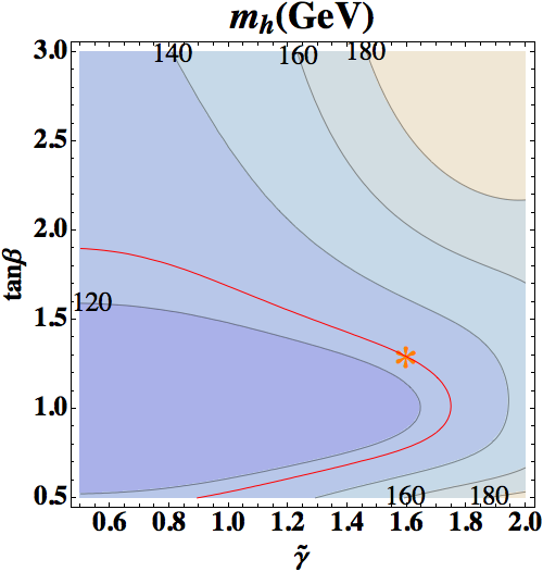
The variation of $m_{h}$ in the $g_{\rm PQ}-\tan\beta$ and $\delta-\frac{f_{S}}{f_{\rm PQ}}$ planes is shown in Fig. 1, where the loop corrections from the MSSM mediated by stop and sbottom quarks have been included. We see that $m_{h}=125$ GeV can be easily accommodated without heavy or split stops. The behavior of $m_{h}$ is mainly controlled by tree-level effects. With fixed $g_{\rm PQ}$, $m_{h}$ has a minimal value for $\tan\beta\sim 1$ where the MSSM tree-level contribution is minimized. If $\tan\beta$ is fixed, $m_{h}$ becomes larger as $g_{\rm PQ}$ increases. $\delta$ and $f_{S}/f_{\rm PQ}$ provide a set of measures of the D-term and F-term corrections to $m_{h}$. These features can be easily understood using Eq. (8) and Eq. (5).

The effective Lagrangian of $h\rightarrow\gamma\gamma$ can be written as

where $I$ is a constant parameterizing the effective $h\gamma\gamma$ coupling. Any particles coupled with it must get a mass from the Higgs VEVs. The effective coupling shown in Eq. 9 is induced by charged particles which can couple with the Higgs boson. If the Higgs mass is smaller than that of the charged particles mediating the $h\gamma\gamma$ loop, the effective $h\gamma\gamma$ coupling can be calculated through the photon self-energy corrections [34, 35]. In the SM, there is only one Higgs doublet and the neutral component can be written as $H_{\rm SM}=(h+v_{\rm EW})/\sqrt{2}$. We have

where for bosonic degrees of freedom ${\cal M}_{k}^{2}$ is the mass matrix and for fermionic degrees of freedom ${\cal M}_{k}^{2}={\cal M}_{k}^{\dagger}{\cal M}_{k}$, with $k$ running over all mass matrices of charged bosonic and fermionic particles. $b_{k}$ is the coefficient in the beta function of QED, with $b_{1/2}=\frac{4}{3}Q_{f}^{2}$ for Dirac fermion, $b_{1}=-7Q_{v}^{2}$ for charged vector boson, and $b_{0}=\frac{1}{3}Q_{S}^{2}$ for charged scalar. In the SM, the main contributions come from top quark and $W$ boson. They have opposite signs. The $W$ boson contribution dominates over that of the top quark, and hence controls the sign of the $h\gamma\gamma$ coupling in the SM [35].

In the case of SUSY, there are two Higgs doublets, which makes the discussion complicated. The effective coupling can be modified to

Usually there is no fixed relation between the Higgs alignment $\alpha$ and VEV alignment $\beta$. In this paper, we concentrate on the scenarios in which the decays of the SM-like Higgs boson to $WW$, $ZZ$, $b\bar{b}$, $\tau\bar{\tau}$ channels are similar to that of the SM Higgs, and only the loop-dominant $h\rightarrow\gamma\gamma$ channel is modified. In comparison with the SM, the decay amplitude of $h\rightarrow b\bar{b}$ and $h\rightarrow WW/ZZ$ in MSSM are scaled by a factor of $\frac{\cos\alpha}{\sin\beta}$ and $\sin(\beta-\alpha)$, respectively. If $\beta-\alpha\approx\pi/2$, their decay widths are approximately equal to the SM ones. The contributions from the $W$ boson and top quark to $h\rightarrow\gamma\gamma$ is also similar to the SM one, which give $I_{W}\approx-2.1$ and $I_{\rm top}\approx 0.5$. The effective Lagarangian is reduced to the one in Eq. (10).

If the masses of the intermediate particles are smaller than half of the Higgs mass, they can be pair-produced via the Higgs decay. Treating the exotic induced $h\rightarrow\gamma\gamma$ coupling as point-like, as described by the effective Lagrangian in Eq. (9), is not appropriate. For $m_{h}=125$ GeV, the current lower bounds on the mass of the charged new particles are around 100 GeV [37]. Therefore, the effective theory description is always valid. For relatively light mediators, there are corrections to $b_{k}$’s up to the order of $m_{h}^{2}/4m_{\rm mediator}^{2}$. These corrections are small and will not change the conclusions reached in this section qualitatively. The exact formulae can be found in Ref. [35, 36], and they will be used in our numerical calculations in the next section.

From Eq. (11), we can see that the sign of the effective coupling is determined by two factors, the $\beta$-function $b_{k}$ and the derivatives of the mass matrix with respect to the Higgs VEVs. For fermions and complex scalars, $b_{k}$ is positive. In the SM, the fermions have ${\cal M}^{\dagger}{\cal M}\sim|y|^{2}v_{u,d}^{2}$, where $y$ is Yukawa coupling. Therefore, the derivative is always positive. For general exotic fermions, however, there can have vector-like mass terms. The derivative can be either positive or negative. For exotic scalars, in SUSY models, generally they can obtain mass from the Higgs VEVs in two ways. One is from the F-term of the exotic superfield. In this case the derivatives are always positive. The other is from the $A$-term between the exotics and the Higgs boson. In this case, the derivatives can be either positive or negative. In the next section, we will discuss benchmark models of these two scenarios.

To enhance the $h\rightarrow\gamma\gamma$ signal rate significantly, the contribution from the exotic states needs to be comparable with the SM contributions from $W$ boson and top quark. As a result, either the fermion or the scalar mediators should be light. Since these particles carry EW charges, they may non-trivially contribute to the observables of the EWPT. Therefore, the EWPT can provide strong constraints on the models discussed here. These potential contributions include oblique and non-oblique corrections. We will focus on the former, because the non-oblique ones are sensitive to the couplings of the mediators with the SM fermions, which can be taken to be small. The oblique corrections represent new physics effects in the vacuum polarization of the SM gauge bosons, and are usually parameterized by the Peskin-Takeuchi parameters, $S$, $T$ and $U$ [39]. The $U$ parameter is not very sensitive to new physics, and only receives contributions from dimension-eight operators or above, so we will not discuss it in the following analysis. The $U(1)_{\rm PQ}$ gauge boson can also have non-trivial contributions to the EWPT observables, via its mixing with the $Z$ boson. This has been discussed extensively (e.g., see [38]). For the scenarios discussed in this paper, the $Z-Z^{\prime}$ mixing is small because the $U(1)_{\rm PQ}$ scale is relatively high while its gauge coupling is not very large. Such contributions therefore are well under control.

In this section, we construct an explicit model which realizes the ideas discussed in the previous sections. $U(1)_{\rm PQ}$ with only the SM matter content is anomalous. There are many possible choices of spectators to cancel this anomaly. However, new EW doublets and color triplets carrying $U(1)_{\rm PQ}$ charges are always required for canceling the $SU(2)^{2}\times U(1)_{\rm PQ}$ and $SU(3)^{2}\times U(1)_{\rm PQ}$ anomalies, respectively. As an illustration, let us consider a model given in Table 1. Other possible implementations have qualitatively similar features. The superpotential of this model is given by

with $p,q=1,2$. ${\bf W_{\rm H}}$ is presented in Eq. (3). We have only displayed explicitly the interactions most relevant for our discussion on the modification of the $h\gamma\gamma$ effective coupling. ${\bf W_{\rm Y}}$ has the same form as the MSSM Yukawa couplings, but with the replacements ${\bf H_{u}\leftrightarrow D_{p}}$ and ${\bf H_{d}\leftrightarrow D_{q}^{c}}$. ${\bf W_{\rm S}}$ includes all terms with only the PQ symmetry breaking fields $({\bf S,S^{c},S_{1},S_{1}^{c},S_{2}})$. ${\bf W_{\rm LQ}}$ contains the interactions involving the color triplets ${\bf T_{1,2,3}^{(c)}}$. It has the coupling of the form ${\bf STT^{c}}$, and $\kappa^{rs}{\bf L_{r}Q_{s}T_{3}}+\kappa^{rsp}{\bf\bar{N}_{r}\bar{u}_{s}T_{p}}$ with $r,s=1,2,3$. After the $U(1)_{\rm PQ}$ symmetry is broken, $({\bf T_{r},T_{s}^{c}})$ and $({\bf D_{p},D_{q}^{c}})$ obtain vector-like masses by coupling with the supermultiplet ${\bf S}$. An important feature is that $({\bf T_{r},T_{s}^{c}})$ and $({\bf D_{p},D_{q}^{c}})$ decay into the SM particles via the interactions in ${\bf W_{\rm LQ}}$ and ${\bf W_{\rm Y}}$, respectively. This can help avoid the overproduction of the exotic particles in the Universe. From the choice of the $U(1)_{\rm PQ}$ charges displayed in Table 1, the only renormalizable couplings between the color triplets and the Higgs bosons are of the form ${H\tilde{q}\tilde{\ell}\tilde{T}}$ or ${HH\tilde{T}\tilde{T}}$. ${H\tilde{q}\tilde{\ell}\tilde{T}}$ will not contribute to the Higgs decay directly. Furthermore, they can be suppressed by choosing small leptoquark-type couplings. ${HH\tilde{T}\tilde{T}}$ will enter $hgg$ effective coupling. However, this contribution can be small if the color triplets is heavy, $m_{\rm T}\sim$ TeV. For these reasons, we will assume that the triplets are heavy and would not discuss them further in this section.

Since the EWPT may give strong constraints on our scenario, we begin with a more general discussion on this issue before presenting the benchmark models. The T parameter is a measure of the breaking of the custodial symmetry, $SU(2)_{c}$. Apart from the mixing between $Z$ and $Z^{\prime}$, in general, there are two contributions which break $SU(2)_{c}$ explicitly. One is from the Yukawa coupling between the exotics and the Higgs fields in the superpotential, such as the difference between the ${\bf H_{u}D_{p}X^{c}}$ and ${\bf H_{d}D_{p}N^{c}}$ couplings, and the corresponding A-terms. In this paper, we choose to preserve the explicit $SU(2)_{c}$ by choosing the relevant Yukawa couplings to be equal. Therefore, instead of four independent Yukawa couplings, we have two, $\gamma_{X^{c}}^{p}=\gamma_{N^{c}}^{p}=\tilde{\gamma}$ and $\gamma_{X}^{q}=\gamma_{N}^{q}=\bar{\gamma}$, and for the corresponding A-terms, we have $A_{X^{c}}^{p}=A_{N^{c}}^{p}=A_{\tilde{\gamma}}$ and $A_{X}^{q}=A_{N}^{q}=A_{\bar{\gamma}}$. We note that certain fine-tuning is necessary in making this choice, as these couplings also receive one-loop corrections proportional to the explicit $SU(2)_{c}$ breaking SM Yukawa couplings. Another contribution to the T parameter comes from the difference between $v_{u}$ and $v_{d}$, which breaks $SU(2)_{c}$ spontaneously. Of course, we can find parameter space where the two contributions cancel with each other. To avoid severe fine-tuning, the bulk of parameter space with such cancellation should not have large explicit or spontaneous $SU(2)_{c}$ violation. Therefore, it should not be very different from the limit that we are considering.

Two benchmark points are presented in Table 2 and Table 3. The parameter $\delta$, defined right after Eq. (7), controls the corrections to the Higgs sector via the $U(1)_{\rm PQ}$ D-terms and is assumed to be sizable for both benchmark points. In the first benchmark, the lightest charged ($\psi_{1}^{c}$) and neutral ($\psi_{1}^{0}$) fermion spectators are light. They have a large coupling to the Higgs fields, for enhancing the di-photon signal rate. To get a small $\Delta T$, the spontaneous breaking needs to be small. Hence, $\tan\beta\approx 1$ is required. For the second benchmark point, where one of the charged scalar is light and couples to the Higgs fields with large $A$ terms (again for enhancing the di-photon signal rate), there is an accidental cancelation which leads to $\Delta T$ to be a few times smaller than its natural value. A detailed discussion of this accidental cancelation can be found in Appendix B. Therefore, even in the case of large $\tan\beta$, the $T$ parameter can still be within the experimental limit.

In addition, although the doublets $({\bf D_{p},D_{q}^{c}})$ are vector-like under the EW gauge symmetry and their fermionic components have a degenerated mass spectrum, the $S$ parameter can still receive non-zero corrections. This is because $({\bf D_{p},D_{q}^{c}})$ mix with $({\bf X,X^{c}})$ and $({\bf N,N^{c}})$, while the latter violate the weak isospin (recall that the $S$ parameter preserves the custodial but measures the violation of the weak isospin).

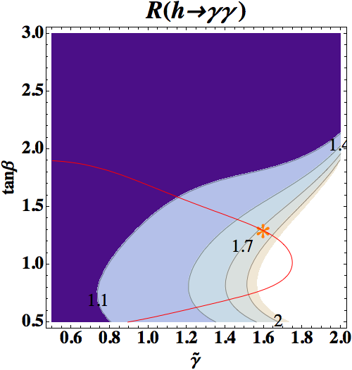
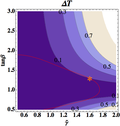
The dependence of $m_{h}$, $R(h\rightarrow\gamma\gamma)$, $\Delta S$ and $\Delta T$ on $\tilde{\gamma}=\bar{\gamma}$ and $\tan\beta$ in the first benchmark is shown in Fig. 2. As is expected, with a fixed $\tan\beta$, $R(h\rightarrow\gamma\gamma)$ tends to be enhanced for a larger $|\tilde{\gamma}|$; and with a fixed $\tilde{\gamma}$, $\Delta T$ tends to be smaller while $\tan\beta$ is close to 1. From the right plot on the first row of Fig. 2, we can see that the correction to the rate of $h\rightarrow\gamma\gamma$ also has a maximum at $\tan\beta=1$ with fixed $\tilde{\gamma}$. We can understand this from the form of the mass matrix of charged fermionic exotics,

where $M_{D}$ and $M_{X}$ are the vector-like mass for the doublet and charged singlet exotics, respectively. Then, we can get

Since we are interested in the region where $\alpha\approx\beta-\pi/2$, we have $\cos(\alpha+\beta)\approx\cos(2\beta-\pi/2)$, which peaks at $\beta=\pi/4$. Therefore, from Eq. (11), we can see that the correction to $I$ reaches its maximum at $\tan\beta=1$.

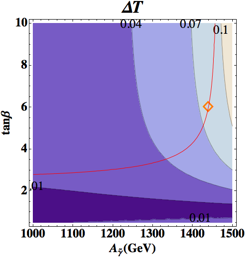
The dependence of $m_{h}$, $R(h\rightarrow\gamma\gamma)$, $\Delta S$ and $\Delta T$ on $A_{\tilde{\gamma}}$ and $\tan\beta$ in the second benchmark is shown in Fig. 3. In this region, since the contribution from $A$ terms dominates over the ones from the Yukawa couplings, the loop correction to Higgs mass from exotics is negative. Therefore, from the first plot in Fig. 3, we can see that $m_{h}$ becomes smaller with larger $A_{\tilde{\gamma}}$. For the correction to the rate of $h\rightarrow\gamma\gamma$, in the region where $A_{\tilde{\gamma}}^{2}>A_{\bar{\gamma}}^{2}$, the charged scalar exotics mainly couple to the Higgs through $H_{u}$ and therefore the correction to the $h\rightarrow\gamma\gamma$ rate behaves similarly to up-type quarks. As a result, the relevant part of the mass matrix of the charged exotics in this limit can be reduced to

from which we can get

where the relation $\cos\alpha\approx\sin\beta$ is used. Therefore, we can see that in this region the correction to the rate of $h\rightarrow\gamma\gamma$ goes up slowly with $\tan\beta$ which is shown in the region $A_{\tilde{\gamma}}$ around 1500 GeV in Fig. 3, where $A_{\bar{\gamma}}$ is fixed to be 1000 GeV. In the region $A_{\tilde{\gamma}}=A_{\bar{\gamma}}$ the dependence of the correction to $h\rightarrow\gamma\gamma$ on $\tan\beta$ is more complicated, and numerical simulation shows that the dependence is not monotonic, as shown in Fig. 3. For the contributions to the $T$ parameter, because of the accidental cancelation discussed in Appendix B, $\Delta T$ is typically small, while $\tan\beta\sim 1$ can bring a further suppression.

Motivated by the discovery of a $\sim 125$ GeV Higgs boson in the CMS and ATLAS experiments, we study the possibility of lifting the tree-level mass of the SM-like Higgs boson in MSSM extended by an extra $U(1)$ gauge symmetry. For definiteness, we focus on the scenarios with a gauged $U(1)_{\rm PQ}$ symmetry which can also be connected to a possible solution to the $\mu$ problem in the MSSM. We limit ourselves to the parameter region in which the softly SUSY-breaking scale is below the $U(1)_{\rm PQ}$ breaking scale, $f_{\rm PQ}>\Lambda_{\rm soft}\sim\Lambda_{\rm EW}$. In this case, we can work in the framework of effective theory with only the axion supermultiplet. We explicitly demonstrate that non-trivial corrections of the $U(1)_{\rm PQ}$ D-term to the Higgs physics necessarily require sizable softly SUSY breaking effects in the PQ symmetry-breaking sector. In particular, a correction $\sim\mathcal{O}(10)$ GeV to the Higgs mass at the tree level can be achieved for $f_{\rm PQ}\sim\mathcal{O}(1)$ TeV and $\frac{\Lambda_{\rm soft}}{f_{\rm PQ}}\sim\mathcal{O}(0.1)$. In addition to the Higgs mass, the LHC data also reveals a tantalizing hint of a significantly enhanced di-photon signal rate. We show that this feature can be accommodated in this scenario. Gauging the $U(1)_{\rm PQ}$ symmetry necessarily requires the charged exotics for anomaly cancellation. If they happen to be light and have sizable couplings with the Higgs boson, the di-photon signal rate can be significantly enhanced. With the bounds from the EWPT considered, we identify two benchmark scenarios where a light charged exotic fermion and scalar plays a crucial role in modifying the $h\gamma\gamma$ effective coupling, respectively.

Testing this scenario at the LHC is relatively difficult. The first signal is probably still from the modified decays of the SM-like Higgs boson. A confirmation of the enhanced di-photon signal rate would provide a potential evidence for this scenario. In this case, it is obviously important to search for the light charged exotic mediators directly at the LHC. These exotics can be produced through the processes of weak interaction and then decay into the SM particles via the interactions described in the superpotential $\bf W_{Y}$. Their signals are similar to that of the Higgsinos, or sleptons. With the accumulation of the data, we should be able to probe these exotics. Of course, it is also possible to search for the leptoquark-type exotics $\bf T_{1,2,3}$, which are required for cancelling the $SU(3)^{2}\times U(1)_{\rm PQ}$ anomaly. Although not directly related to the modification of the Higgs di-photon decay channel, these colored particles should not be too heavy since their mass is generated through PQ symmetry breaking. They can be pair-produced via QCD processes at the LHC, with leptoquark-like signals. We will leave these studies to a future work.

Although our study is mainly done in the context of a specific model, the lessons we have learned are fairly general. The two benchmarks are representatives of large classes of models in which an enhancement of the $h\rightarrow\gamma\gamma$ signal rate does not lead to a violation of the EWPT constraints. The first benchmark contains four $SU(2)_{L}$ doublets and two charged singlets for the sake of anomaly cancelation. This is only a little larger than the minimal model. As discussed in Sec. IV, for the corrections from fermionic exotics to have the same sign as the W boson contribution, the mass of the fermionic exotics must have two sources. One is chiral, coming from Yukawa like couplings with Higgs fields. At the same time, a Dirac mass term is necessary. Therefore, we at least need to introduce two doublets. Moreover, to avoid explicit breaking of the custodial $SU(2)_{c}$, we must at least introduce two singlets. The mass matrices of the fermionic charged exotics can always be written in the form of Eq. (13). Hence, the discussions for the correction to Higgs to di-photon decay rate made in Sec. V are in general applicable. The second benchmark is a very special case in which a charged scalar can do the job. Another similar example in this class is the light stau scenario in the MSSM [3]. We see that, due to the constraints from the EWPT, a certain amount of fine tuning is unavoidable in models with an enhanced $h\gamma\gamma$ effective coupling. This implies that if such an enhancement is confirmed, it would point us to a new direction of model building not completely guided by the reduction of such fine-tuning. If only the $h\rightarrow\gamma\gamma$ signal rate is enhanced while the other ones are not modified, the new exotic states will carry the EW quantum numbers only. Their collider signals are similar to that of the EW-ino and the slepton. Hence, it would be challenging to search, unless they are part of a long decay chain starting with some colored states.

Acknowledgments

H.A. is supported by the Government of Canada through NSERC and by the Province of Ontario through MEDT. T.L. is supported by the DOE Grant DE-FG02-91ER40618 at U. California, Santa Barbara. L.T.W. is supported by the NSF under grant PHY-0756966 and the DOE Early Career Award under grant DE-SC0003930. T.L. would thank D. Morrissey for useful discussions.

References

- [1] https://cms-docdb.cern.ch/cgi-bin/PublicDocDB/RetrieveFile?docid=6125&filename=CMS_4July2012_Incandela.pdf
- [2] https://cms-docdb.cern.ch/cgi-bin/PublicDocDB/RetrieveFile?docid=6126&filename=Higgs-CERN-seminar-2012.pdf
- [3] M. Carena, S. Gori, N. R. Shah and C. E. M. Wagner, JHEP 1203, 014 (2012) [arXiv:1112.3336 [hep-ph]];
- [4] N. D. Christensen, T. Han and S. Su, arXiv:1203.3207 [hep-ph].
- [5] P. Draper, P. Meade, M. Reece and D. Shih, Phys. Rev. D 85, 095007 (2012) [arXiv:1112.3068 [hep-ph]].
- [6] J. Cao, Z. Heng, J. M. Yang, Y. Zhang and J. Zhu, JHEP 1203, 086 (2012) [arXiv:1202.5821 [hep-ph]].
- [7] J. L. Feng and D. Sanford, arXiv:1205.2372 [hep-ph].
- [8] K. Hagiwara, J. S. Lee and J. Nakamura, arXiv:1207.0802 [hep-ph].
- [9] N. D. Christensen, T. Han and T. Li, arXiv:1206.5816 [hep-ph].
- [10] A. Arbey, M. Battaglia, A. Djouadi and F. Mahmoudi, arXiv:1207.1348 [hep-ph].
- [11] R. Benbrik, M. G. Bock, S. Heinemeyer, O. Stal, G. Weiglein and L. Zeune, arXiv:1207.1096 [hep-ph].
- [12] D. A. Vasquez, G. Belanger, C. Boehm, J. Da Silva, P. Richardson and C. Wymant, arXiv:1203.3446 [hep-ph].
- [13] U. Ellwanger, JHEP 1203, 044 (2012) [arXiv:1112.3548 [hep-ph]].
- [14] L. J. Hall, D. Pinner and J. T. Ruderman, JHEP 1204, 131 (2012) [arXiv:1112.2703 [hep-ph]].
- [15] P. Langacker, Rev. Mod. Phys. 81, 1199 (2009) [arXiv:0801.1345 [hep-ph]].
- [16] P. Batra, A. Delgado, D. E. Kaplan and T. M. P. Tait, JHEP 0402, 043 (2004) [hep-ph/0309149]. A. Maloney, A. Pierce and J. G. Wacker, JHEP 0606, 034 (2006) [hep-ph/0409127]; Y. Zhang, H. An, X. -d. Ji and R. N. Mohapatra, Phys. Rev. D 78, 011302 (2008) [arXiv:0804.0268 [hep-ph]].
- [17] R. D. Peccei and H. R. Quinn, Phys. Rev. Lett. 38, 1440 (1977).
- [18] J. E. Kim and H. P. Nilles, Phys. Lett. B 138, 150 (1984).
- [19] J. E. Kim, H. P. Nilles and M. -S. Seo, arXiv:1201.6547 [hep-ph].
- [20] M. S. Carena, S. Heinemeyer, C. E. M. Wagner and G. Weiglein, hep-ph/9912223.
- [21] M. Carena, S. Gori, N. R. Shah, C. E. M. Wagner and L. -T. Wang, arXiv:1205.5842 [hep-ph].
- [22] M. Carena, P. Draper, T. Liu and C. Wagner, Phys. Rev. D 84, 095010 (2011) [arXiv:1107.4354 [hep-ph]].
- [23] A. Azatov, S. Chang, N. Craig and J. Galloway, arXiv:1206.1058 [hep-ph]; K. Blum, R. T. D’Agnolo and J. Fan, arXiv:1206.5303 [hep-ph].
- [24] M. Carena, I. Low and C. E. M. Wagner, arXiv:1206.1082 [hep-ph].
- [25] B. Batell, S. Gori and L. -T. Wang, JHEP 1206, 172 (2012) [arXiv:1112.5180 [hep-ph]].
- [26] A. Arhrib, R. Benbrik, M. Chabab, G. Moultaka and L. Rahili, JHEP 1204, 136 (2012) [arXiv:1112.5453 [hep-ph]].
- [27] A. Arhrib, R. Benbrik and N. Gaur, Phys. Rev. D 85, 095021 (2012) [arXiv:1201.2644 [hep-ph]].
- [28] K. Blum and R. T. D’Agnolo, arXiv:1202.2364 [hep-ph].
- [29] C. Collaboration [CMS Collaboration], arXiv:1202.1489 [hep-ex].
- [30] B. Bellazzini, C. Csaki, J. Hubisz, J. Shao and P. Tanedo, JHEP 1109, 035 (2011) [arXiv:1106.2162 [hep-ph]].
- [31] P. Draper, T. Liu, C. E. M. Wagner, L. T. M. Wang and H. Zhang, Phys. Rev. Lett. 106, 121805 (2011) [arXiv:1009.3963 [hep-ph]].
- [32] G. Marandella, C. Schappacher and A. Strumia, Nucl. Phys. B 715, 173 (2005) [hep-ph/0502095].
- [33] M. Dine, N. Seiberg and S. Thomas, Phys. Rev. D 76, 095004 (2007) [arXiv:0707.0005 [hep-ph]];
- [34] J. R. Ellis, M. K. Gaillard and D. V. Nanopoulos, Nucl. Phys. B 106, 292 (1976).
- [35] M. A. Shifman, A. I. Vainshtein, M. B. Voloshin and V. I. Zakharov, Sov. J. Nucl. Phys. 30, 711 (1979) [Yad. Fiz. 30, 1368 (1979)].
- [36] V. Barger and R. J. N. Phillips, ”COLLIDER PHYSICS”, ISBN-9780201149456, 1987.
- [37] P. Achard et al. [L3 Collaboration], Phys. Lett. B 580, 37 (2004) [hep-ex/0310007].
- [38] J. Erler, P. Langacker, S. Munir and E. Rojas, JHEP 0908, 017 (2009) [arXiv:0906.2435 [hep-ph]]; M. E. Peskin and J. D. Wells, Phys. Rev. D 64, 093003 (2001) [hep-ph/0101342].
- [39] M. E. Peskin and T. Takeuchi, Phys. Rev. Lett. 65, 964 (1990).
- [40] N. Arkani-Hamed, M. Dine and S. P. Martin, Phys. Lett. B 431, 329 (1998) [hep-ph/9803432].