Mg ii Absorption at with Magellan / FIRE.
II: A Longitudinal Study of H i, Metals, and Ionization in
Galactic Haloes
Alternate Affiliation: This paper includes data
gathered with the 6.5 meter Magellan Telescopes located at Las
Campanas Observatory, Chile
Abstract
We present a detailed study of H i and metals for 110 Mg ii absorption systems discovered at in the infrared spectra of high redshift QSOs. Using new measurements of rest-frame UV lines from optical spectra of the same targets, we compare the high redshift sample with carefully constructed low redshift control samples from the literature to study evolutionary trends from ( Gyr). We observe a significant strengthening in the characteristic for fixed Mg ii equivalent width as one moves toward higher redshift. Indeed at our sample’s mean =3.402, all Mg ii systems are either damped Ly absorbers or sub-DLAs, with % of systems exceeding the DLA threshold (compared to % at =0.927). We set lower limits on the metallicity of the Mg ii systems where we can measure H i; these results are consistent with the full DLA population. The classical Mg ii systems (Å), which preferentially associate with sub-DLAs, are quite metal rich at Solar. We applied quantitative classification metrics to our absorbers to compare with low redshift populations, finding that weak systems are similar to classic Mg ii absorbers at low redshift. The strong systems either have very large Mg ii and Fe ii velocity spreads implying non-virialized dynamics, or are more quiescent DLAs. There is tentative evidence that the kinetically complex systems evolve in similar fashion to the global star formation rate. We speculate that if weaker Mg ii systems represent accreting gas as suggested by recent studies of galaxy-absorber inclinations, then their high metal abundance suggests re-accretion of recently ejected material rather than first-time infall from the metal-poor IGM, even at early times.
Subject headings
Galaxies: evolution—Galaxies: halos—Galaxies: high-redshift—Infrared: general—intergalactic medium—quasars: absorption linesI. Introduction
For decades, Mg ii quasar absorption lines have been used to probe the gas distribution in galactic haloes in a largely dust extinction and luminosity-independent manner [80, 32, 77, 61, 73, 42, 54, 37, e.g., ]. Despite this rich literature, the spatial structure and dynamical history of the gas giving rise to Mg ii absorption are not fully understood. Several important clues have surfaced through the aforementioned studies, and (broadly speaking) they point to two plausible mechanisms. The first possibility is that Mg ii traces cool clumps embedded in hot galactic outflows [87, 11, 79, 26, 37, 59, 44, 40, e.g., ]. The second postulates that Mg ii absorbing structures are a manifestation of gravitational and gas accretion processes, perhaps even through recycled and metal-enriched winds [15, 16, 34, 30, e.g., ].
The outflow hypothesis is supported by low redshift studies showing a connection between Mg ii absorption and star formation. For example, Zibetti et al. [87] demonstrated that strong absorber correlates with blue host galaxy color, using a sample of 2800 strong Mg ii systems () at low redshifts (), a result later corroborated by Lundgren et al. [37].
More directly, Weiner et al. [79] observe blueshifted (and hence outflowing) foreground Mg ii absorption in the stacked spectra of star forming galaxies. Follow up work by Rubin et al. [59] verifies this trend and establishes a correlation between Mg ii rest-frame equivalent width and star formation rate (SFR). Nestor et al. [41] studied two ultra-strong Mg ii absorbers ( = 3.63 and 5.6 Å) in detail, finding that they were associated with galaxies of unusually high specific star formation rate at their respective masses and redshifts.
Further evidence of a Mg ii-wind connection may be found from studying statistical clustering of Mg ii systems relative to nearby galaxies. Gauthier et al. [26], following up on the work of Bouché et al. [10] and Lundgren et al. [37], find a anti-correlation between Mg ii rest-frame equivalent width and galaxy halo mass by cross-correlating luminous red galaxies with Mg ii absorbing systems from SDSS-DR5 at . Although the anti-correlation is weak, in conjunction with studies showing a strong correlation between and velocity spread [22, 39] it suggests that the individual Mg ii systems are not virialized.
While these and other studies [11, 44, 40, e.g., ] have advocated outflows as a mechanism for creating Mg ii absorption, there is also evidence suggesting that many Mg ii systems do not originate in winds. For example, Chen et al. [15] find little evidence for correlation between absorber strength and galaxy colors using a galaxy-selected sample of Mg ii systems, in direct contrast to Zibetti et al. [87]. Similar galaxy-selected samples of weaker absorbers confirm this result [34, 30]. Moreover, Chen et al. [16] demonstrate with a sample of 47 weaker (mostly Å) systems at that the extent of the Mg ii halo correlates only weakly with specific star formation rate and increases with galaxy stellar mass. The authors suggest that this may be evidence that Mg ii absorbers reside in infalling clouds that later fuel star formation.
Recently, Bordoloi et al. [9] and Kacprzak et al. [30] have explored the connection between absorber strength and galaxy-absorber projected inclination, finding evidence for both co-planar and bipolar distributions of absorbing gas. While the outflow hypothesis naturally predicts winds escaping perpendicular to galactic disks as found by Bordoloi et al. [9], the analysis of Kacprzak et al. [30] indicates that co-planar gas exists around some systems, as might be found in accreting streams and filaments.
Collectively, these studies seem to suggest that Mg ii absorbers fall into at least two categories, as outlined in Kacprzak & Churchill [29]. Loosely speaking, weaker absorbers are more likely to possess disk-like kinematics and trace infalling or recycled material. The stronger absorbers have non-gravitational kinematics and are more likely to trace winds. However all of these results were derived from relatively low redshift () systems that postdate the star formation peak of the universe at . Since star formation plays an important role in this discussion, the evolution of Mg ii absorbers through the rise and fall of the SFR history provides a diagnostic tool for evaluating the two-sample paradigm. But Mg ii absorption at these higher redshifts falls into the near infrared, where atmospheric OH emission and telluric absorption make large systematic surveys much more difficult.
In Matejek & Simcoe (2012; hereafter, Paper I), we presented the first statistically characterized sample of Mg ii absorption lines at , taken from the spectra of 46 QSO sightlines observed with Magellan/FIRE. We located 110 intervening Mg ii systems (plus one proximate system) ranging in rest equivalent width from to and in redshift from to . The weaker systems’ linear density is statistically consistent with no evolution from to (a span of over 8 Gyr). In contrast, the stronger systems’ linear density increases three-fold until before declining again towards higher redshifts. The evolutionary behavior of these strong systems suggests that there may indeed be a connection between star formation and the strong end of the Mg ii population.
The present study follows up the initial survey of Paper I by studying the full properties of each individual Mg ii system in detail. Combination of our data with multiple low redshift samples yields a longitudinal view of H i and metals in Mg ii-selected absorbers over a wide baseline in redshift. For the sample, we also benefit from the shifting of vacuum ultraviolet lines including H i, C iv, and other baseline metal transitions into optical wavelengths. This allows us to leverage a large assortment of ground based measurements to study the systems’ chemistry and ionization.
Our goals in investigating the internal properties of individual Mg ii systems over a wide time baseline are: (1) to determine whether the lack of evolution in for weak systems (found in Paper I) reflects a truly non-evolving population or rather masks internal evolution that is manifested in other observables; (2) to determine whether the dichotomy between outflowing and infalling Mg ii is revealed in properties other than , such as chemical composition or H i column density; and (3) to develop a taxonomy for high redshift systems and determine how these relate to low-redshift classes of Mg ii systems and in what proportions.
Section II describes our sample data. In Section III, we describe our data analysis techniques, detailing our calculations of metal rest equivalent widths, column densities, metallicities, and velocity spreads. In Section IV, we present our main science results, including all measured values, correlations, and Kaplan-Meier/K-S test results.
In Section V, we discuss the implications of these results to the broader question of Mg ii absorption. In particular, in Section V.1 we apply a quantitatively derived taxonomy based upon that in Churchill et al. [18] and study the evolution of various classes. In Section V.2, we compare the Mg ii-selected DLA population to the full population. In Section V.3 we discuss possible interpretations resulting from our chemical composition study.
Throughout this paper we use a CDM cosmology with , , and km s-1 Mpc-1.
II. Data Sample
Our overall analysis contains a large number of heterogeneous subsamples both observed by our group and collected from the literature, yielding a total sample of over 17,500 absorbers ranging from . In Sections 2.1 and 2.2 we describe the infrared and optical observations of the systems obtained by our group for the primary survey. Section 2.3 and associated subsections describe the numerous samples collected from the literature that serve as our low redshift control.
II.1. The FIRE Mg ii sample
Paper I provides the full details of the acquisition and reduction of this data. Briefly, we observed 46 QSO sightlines with Magellan/FIRE [69, 70], between 2010 June and 2011 April. FIRE is a single object, prism cross-dispersed infrared spectrometer with a FWHM spectral resolution of km s-1. The survey quasars have emission redshifts between 3.55 and 6.28, and were predominantly chosen from the SDSS DR7 quasar catalog [66], although some bright, well-known objects not in the SDSS catalog were also included.
We reduced the data using a custom-developed IDL pipeline named FIREHOSE that evolved from the optical echelle reduction software package MASE [7]. We corrected for telluric absorption features by obtaining spectra of A0V stars at comparable observing times, air masses and sky positions as our observed QSOs and employing the xtellcor software package [21]. The final spectra ranged in median signal-to-noise ratio per pixel from 4.0 to 47.2, with a median value of 12.9.
Using automated techniques with interactive verification, we identified 110 isolated Mg ii absorbers ranging in rest equivalent width from to and in redshift from to . We carefully characterized both the sample’s completeness as a function of and also its expected false positive rate, adjusting our linear density calculations accordingly. Using the supporting optical data compiled for the present paper, we have identified two systems from Paper I likely to fall among these false positives, discussed below. As expected, they are among the weakest systems in the original sample ( Å ). These absorbers are left out of statistical analysis for both papers because of incompleteness at Å; they are also identified accordingly in all tables presented here.
II.2. Supporting Optical Spectra
Rest-frame UV transitions such as Ly and numerous carbon, silicon, and aluminum transitions are redshifted into the optical window for absorption systems, making these measurements easily accessible from the ground. We obtained new or archival optical spectra for 39 of the 46 QSO sightlines in our survey using data from four different instruments. Table 1 provides a full description of the optical data, including exposure times and wavelength coverages. We limited our metal line search to regions redward of each QSO’s Ly emission peak, and only searched for Ly absorption redward of the Lyman break for the highest redshift Lyman limit absorber. These requirements set the minimum search wavelength in all our spectra even when the data extended further to the blue.
II.2.1 Magellan/MagE - 15 spectra
We obtained optical spectra of 15 objects with Magellan/MagE, a single-object echellette [38], between 2009 March and 2011 January. We used a 0.7” slit and observed mostly at low airmass in 0.6” to 0.8” seeing. The spectra were reduced using the MASE pipeline [7]. The 1D spectra range in signal-to-noise per pixel redward of the Ly Forest from 3.5 to 38.5, have a resolution of km s-1, and span Å to 10280 Å.
Representative regions of the MagE spectrum for Q0000-26 are shown at the upper left of Figure 1, which displays all metal lines detected at a 3 level in the FIRE and MagE spectra at . The MagE spectrum for this object has a median signal-to-noise ratio of per pixel redward of the Ly forest.
In the same MagE spectrum, we did not find a Å Mg ii absorber at , where the FIRE and the MagE spectra overlap, as reported in Paper I. Since the MagE spectrum has a higher signal-to-noise ratio in this region, we now regard this as a false positive.

II.2.2 MIKE - 2 spectra
For two sample quasars (BR0353-3820 and BR0418-5723) we had high-resolution optical spectra available from previous studies of C iv for other programs [68]. These were taken with the Magellan Inamori Kyocera Echelle [6, MIKE,], between 2004 and 2006. The MIKE spectra have a resolution of 14 km s-1, span the wavelength range Å to 9400 Å, and have median signal-to-noise ratios per pixel of 43 for BR0353-3820 and 32 for BR0418-5723.
The upper right set of plots in Figure 1 displays all metal lines detected at a 3 level for the absorbing system along BR0353-3820, and includes representative samples of the BR0353-3820 MIKE spectrum.
II.2.3 HIRES - 1 spectrum
Q1422+2309 is a well known gravitationally lensed quasar. 11 1 The lensing galaxy falls at [31], well below the redshift search range for our study. The inclusion of this quasar therefore does not bias our results in this work or in Paper I. We obtained a high ( 40) SNR HIRES [78] optical spectrum of it from A. Songaila’s spectral archive at the University of Hawaii22 2 http://www.ifa.hawaii.edu/users/acowie/spectra/spectra_hires.html. The spectrum, originally published in Ellison et al. [23], has a resolution of 6.6 km s-1 and covers the wavelength range Å to 7300 Å. All metal lines detected at a 3 level for the system along Q1422+2309 found in both its FIRE and HIRES spectra are shown in the bottom left set of plots in Figure 1. The high SNR and resolution of this HIRES spectrum allow us to detect Si ii 1304 absorption of only 7 mÅ. It also revealed a greater velocity width for this system than previously reported in Paper I. The updated and values used in this study are provided in Table 2. (These adjustments do not effect the calculations from Paper I because this system was missed by our automated finder, and therefore was left out of those calculations to avoid overcompensating for incompleteness.)
II.2.4 SDSS - 21 spectra
We downloaded optical counterparts for 21 of the remaining 28 QSO sightlines from the DR7 spectral archives33 3 http://das.sdss.org/www/html/ of the Sloan Digital Sky Survey [43, SDSS,]. These spectra have a resolution of km s-1, a wavelength range of to 9250 Å, and signal-to-noise ratios per pixel that range from 3.2 to 30.1. The lower right set of plots in Figure 1 includes representative samples of the SDSS spectrum of SDSSJ011351 (signal-to-noise 14), displaying all metal lines detected at a 3 level for the absorption system found in both its SDSS and FIRE spectra. In general the SDSS spectra are sensitive only to the stronger metal-line systems, but they are very useful for measuring H i column densities.
II.3. Comparison Samples
Since our primary goal is to study the redshift evolution of Mg ii-selected systems, we must also establish a local control sample. For this purpose we consider four comparison sets: a compilation of previously published low redshift metal absorption lines, new measurements of metal lines from a Mg ii-selected sample of the SDSS DR7, a low redshift HST sample including measurements for Mg ii-selected systems, and a damped Ly (DLA) selected metallicity sample from the literature.
II.3.1 Low Redshift Literature Compilation
We conducted an extensive compilation of low redshift () metal absorption lines previously reported in the literature to complement our high redshift survey [86, 64, 84, 85, 83, 60, 63, 58, 25, 32, 77, 61, 62, 71, 46, 5, 73, 3, 1, 47, 4, 74, 28, 19, 17, 18]. For this exercise, we included only blind searches of QSOs not selected with any prior knowledge about absorption properties. Because we are studying multiple metal and H i transitions for each Mg ii system, we favored surveys that reported all detected transitions, and not simply Mg ii (or Mg ii and Fe ii). In many cases the same object was observed in multiple surveys covering different wavelengths and transitions. To avoid duplication in such instances, we considered absorption systems whose redshifts matched within 250 km s-1 to be the same.
For consistency, we converted all absorption features detected at less than a 5 significance to upper limits and adjusted all reported 3 and 4 upper limits to a 5 level. Unfortunately, most of these surveys do not list upper limits at the expected locations of undetected transitions. This omission becomes important when we attempt to build distribution functions of for each transition using survival analysis. To capture this information in a very conservative way, we estimated upper limits for all unreported transitions that could have been detected in each spectrum given its wavelength bounds. This process is necessarily crude because we did not have access to the original data, but ignoring the effect would bias our distributions to the high side. For each non-detection, we simply assigned an upper limit equal to 5 times the largest error listed for an identified absorption line in that QSO’s spectrum. All lines flagged as blends were also treated as upper limits. These blended upper limits, however, violate the principle of random censorship because their values are dependent upon the actual line strengths, and were therefore omitted from survival statistics [24].
In all, we located 2705 unique absorption systems across the surveys listed above. Of these, 393 had Mg ii 2796 absorption lines detected at more than a 5 significance. Within this Mg ii subset, we threw out 66 systems and 14 proximate systems (which we defined as residing within 10,000 km s-1 of the QSO). This left us with 313 isolated, Mg ii-selected systems in our compilation set. These systems range in redshift from 0.01 to 2.44 and in rest equivalent width from 0.030Åto 5.796Å. Table 3 contains measurements for a selection of these transitions on a system by system basis.
II.3.2 SDSS DR7 Mg ii sample
To augment our low redshift data from the literature, we also searched for multiple metal line transitions coincident with Mg ii systems identified in spectra from the SDSS DR7 (Seyffert, et al., in prep). Many previous Mg ii absorption studies [42, 54, 55] have worked with SDSS spectra, making this a nice comparison set. The SDSS DR7 parent sample includes over 65,000 Mg ii systems discovered by an automated continuum fitting and search algorithm and then interactively inspected for final approval. The details of this process may be found in Seyffert, et al. (in prep) and Cooksey et al. [20].
We only considered the subset of systems from this full set which had the highest possible user-rating on a 4-point scale and observed at a 5 significance. Using these redshifts, we re-fit a selection of metal transitions in an automated fashion, and recorded upper limits where no absorption was detected. The final subset included 17,296 Mg ii absorption systems with and .
Although this sample contains many more systems than the low redshift compilation discussed last section, the SDSS spectra typically have lower signal-to-noise ratios and are largely incomplete for rest equivalent widths . In addition, the automated determination of metal line rest equivalent widths leaves the sample vulnerable to continuum errors, blended lines, and other effects typically spotted and adjusted for during interactive inspection. For these reasons we use the DR7 sample as a supplement to the low redshift comparison set rather than its replacement, despite its large number of systems.
II.3.3 HST Mg ii-selected Sample
One of our chief aims is to characterize the H i properties of Mg ii systems, but at low redshift only a small fraction of all known Mg ii absorbers have H i measurements since the Ly transition may only be observed from space. Rao et al. [57] present the largest such sample, with measurements of 197 systems taken with the Hubble Space Telescope (HST), as part of a search for low redshift DLAs. Their survey pre-selects based on Mg ii strength of known absorbers identified from a broad literature search (the full list is given in their Table 1). Special preference was given to systems with large Fe ii 2600 equivalent width to maximize the yield of DLAs. These Mg ii-selected systems range from 0.116 to 1.645 and 0.300 to 3.264Å. The measurements range from 18.18 to 21.71 cm-2 with a mean error across the sample of 0.087 cm-2.
Because this sample was selected specifically to maximize the probability of uncovering DLAs, it is not a statistically representative collection of random Mg ii systems. However, it is the largest H i+Mg ii compilation known. So, we adopt it below and correct the distribution in postprocessing to make it statistically equivalent to a randomly drawn Mg ii population (Section III.3.3).
II.3.4 Metallicity sample
Another topic of interest is whether the metallicities of Mg ii-selected systems differ from the general population at high redshift. Since most Mg ii-selected systems are DLAs or sub-DLAs, we use Prochaska et al. [53] as a comparison set. The authors provide abundance measurements on 86 DLAs found along 42 QSO sightlines taken with HIRES/Keck and 65 QSO sightlines taken with the echellete on the Echellete Spectrograph and Imager [67, ESI, ]. The DLA absorption redshifts range from 0.613 to 4.282 with a mean of 3.019. These systems were not selected for Mg ii, but constitute a high redshift abundance reference.
III. Analysis
III.1. Mg ii Line Identification
Paper I contains details of the Mg ii line identification algorithm applied to our FIRE data. Briefly, we used an automated continuum fitting algorithm, and then ran a matched filter search using a double Gaussian separated by the Mg ii doublet spacing as a kernel. To mitigate the high false positive rate caused by intermittent telluric absorption features and missubtracted emission lines, we subjected each Mg ii candidate to a set of consistency checks (e.g., within errors). Finally, the surviving candidates underwent a visual inspection before ultimate acceptance. We fit rest equivalent widths to each doublet using boxcar summation between user-defined limits.
III.2. Measurements
III.2.1 Calculating H i Column Densities
For our high-redshift Mg ii systems with H i coverage, we manually fit H i column densities with Voigt profiles using the x_fitdla routine in the XIDL library.11 1 http://www.ucolick.org/xavier/IDL/index.html Since all our measured systems turned out to be either DLAs or sub-DLAs (i.e., above the flat portion of the H i curve of growth), our final fits were not sensitive to the value, and we fixed it at 30 km s-1. This decision was largely a practical consideration, since the QSOs’ high redshifts made it highly likely that unassociated Lyman limit absorbers would obscure the measurements of Ly or higher order transitions.
Toward the low end of the range in our sample, the effect of an uncertain becomes more pronounced, so we account for this in the quoted errors for these systems. The resolution of our optical spectra was typically too low to identify individual subcomponents in each absorption system, so we fit only one H i component except for our HIRES spectrum of Q1422 and two complex systems with wide velocity spreads. Even in these cases, the resolution did not allow us to fit unique H i column densities to the individual components. Lyman limit absorption from systems at higher redshift obscured even the Ly transitions for the majority of our absorption systems; we excluded these from the H i sample.
In all, we were able to measure H i column densities for 33 of the 110 Mg ii systems in Paper I. Plots of these Ly profiles are shown in Figure 2 with their fitted Voigt profiles overplotted. Table 4 lists all the measured H i column densities.
Some surveys from the literature only quote H i equivalent widths, and we wished to compare our results with these as well. We calculated rest equivalent widths by integrating the area under the best fit Voigt profiles. Errors on were conservatively calculated by employing a boxcar summation of the normalized error array where the best fit Voigt profile fell below 10% of the continuum. These rest equivalent widths are stored in Table 5.
As part of this process, we discovered that the putative Mg ii system at toward SDSS0113-0935 (reported in Paper I) exhibited no Ly in its SDSS spectrum even though the data quality and flux level should have allowed such a detection. We therefore consider this system (with Å) a false positive.

III.2.2 Metals
In addition to the Mg ii 2796 and Mg ii 2803 rest equivalent widths calculated in Paper I, we searched redward of the QSOs’ Ly emission peaks in the FIRE and optical spectra for metal transitions at the locations predicted by the Mg ii doublet redshifts. We employed a boxcar method to calculate rest equivalent widths for these lines using interactively-defined limits set to where the flux met the continuum. In some cases, no clear absorption lines existed at the expected locations. In these cases, we estimated an upper limit by boxcar summation of pixels. We made no attempt to disentangle blended lines, treating such collisions as upper limits.
In this way we fit a large assortment of metal transitions including: Mg ii 2796, Mg ii 2803, and Mg i 2852 (Table 2); Fe ii 1608, Fe ii 2344, Fe ii 2374, Fe ii 2382, Fe ii 2586, and Fe ii 2600 (Table 6); Si ii 1260, Si ii 1304, Si iv 1393, Si iv 1402, Si ii 1526, and Si ii 1808 (Table 7); C ii 1334, C iv 1548, and C iv 1550 (Table 8); Al ii 1670, Al iii 1854, and Al iii 1862 (Table 8); and O i 1302 (Table 5).
III.2.3 Kinematic Measurements
We fit velocity spreads for all detected metal lines, except those measured with SDSS spectra (which we omitted because of their low resolution). These velocity spreads were calculated by considering the minimum and maximum wavelengths of the absorption line (as determined by the user-defined equivalent width limits, where the absorption line meets the continuum) and correcting for the instrumental resolution of the spectra. We conservatively set the errors on these velocity spreads to be the greater of 10% and the pixel width divided by .
We also measured the “kinematic spread” for each transition, following the analysis of Churchill et al. [18]. This quantity is defined as the square root of the optical depth-weighted second moment of the velocity difference from the centroid (their Equation 1). Table 9 contains all measured kinematic and velocity spreads for the Mg ii 2796, Fe ii 2600, and C iv 1548 transitions for the FIRE sample. We substituted measurements for other transitions when possible if the main transition could not be measured (e.g., Fe ii 2586 for Fe ii 2600).
III.2.4 Metallicities
We calculated metallicity values or lower limits for the 33 absorption systems with measured H i column densities (Table 4). First, we estimated column densities for all detected metal absorption lines using the apparent optical depth (AOD) method of Savage & Sembach [65], although the corresponding values represent lower limits on column densities for saturated lines. To determine whether an absorption line was saturated, we estimated the rest equivalent width at which the curve of growth becomes non-linear for each metal transition (conservatively setting km s-1). Since we generally do not resolve the absorption complexes into their constituent subcomponents, we used this rest equivalent width threshold as the barrier between saturation (stronger absorption) and non-saturation (weaker). This may overestimate the likelihood of saturation for lines with significant velocity substructure, but it provides the most robust possible lower limit.
For each ion (e.g., Fe ii), we used the average column densities of all non-saturated transitions (e.g., Fe ii 1608, 2344, 2374, 2382, 2586, and 2600) and divided by as determined above. When all metal transitions were saturated, we used the highest value of the lower limit. Finally we normalized to the solar abundance scale of Asplund et al. [2]. We did not apply ionization corrections to the metallicity estimates. This approximation is suitable for DLAs, but may lead to errors at the 0.1-0.3 dex level for lower systems in our sample that would be classified as sub-DLAs [45, see also Section IV.4].
III.3. Normalizing Mg ii Samples for Statistical Comparison
Given the heterogeneous nature of our high redshift and control samples, we exercised special care to create selected subsamples for statistical comparisons. Our goal is to isolate effects that are intrinsically evolving in the source population, and reduce our sensitivity to observational and/or selection biases that differ between samples.
III.3.1 Generating Low and High Redshift Samples
First, we divided the total set of all Mg ii-selected systems from FIRE and the literature compilation with Mg ii 2796 detected at a 5 level into a low redshift and a high redshift sample, separated at . The low redshift compilation set from the literature is predominantly systems and the FIRE set is predominantly systems, so these two samples are roughly exclusive. We formed a separate low redshift set from the SDSS data.
Figure 3 shows the cumulative distribution function (CDF) of Mg ii 2796 rest equivalent width for our low redshift sample (top panel), high redshift sample (middle panel), and the SDSS sample (bottom panel). In each panel, the light gray line includes all identified Mg ii systems, and the dashed black line represents the analytic CDF for an exponential equivalent width distribution (), with appropriate for each respective epoch. For high redshifts we set =0.824, the completeness-corrected value measured in Paper I. For both the low redshift and SDSS DR7 sample, the overplotted exponentials have =0.702, which is the completeness-corrected value from Nestor et al. [42], measured from the SDSS Early Data Release sample. The large underabundance of systems with small rest equivalent width is an indication of incompleteness.

Following past convention from Paper I, we can minimize incompleteness effects by restricting our analysis to systems. The dark gray lines in Figure 3 display the CDFs for this cut, while the solid black curves represent the same analytically calculated CDFs as before, but with this lower limit imposed. The analytic and observed distributions show good agreement for the high and low redshift subsamples. The SDSS DR7 sample still suffers from incompleteness issues below . Rather than slicing all data to (which would result in very few systems at high redshift), we instead forced the SDSS set to fit the analytic CDF by drawing an appropriately weighted subsample from the SDSS parent population. The resulting CDF of this subset is overplotted in Figure 3 as a dotted, dark gray line.

Figure 4 displays histograms of the redshift (upper panel) and rest-frame equivalent width (lower panel) for these lower redshift (light gray line), higher redshift (black line), and SDSS DR7 (dark gray line) samples. The bins for the SDSS DR7 sample are eight times smaller in order to facilitate overplotting. The low , high , and SDSS samples contain 272, 97, and 1975 systems at mean redshifts of 1.128, 3.184, and 1.064, respectively. Table 10 lists the mean redshift, number of detections and upper limits, and minimum and maximum rest-frame equivalent widths for a selection of metal transitions in each sample.
Because our low/high redshift cut was motivated chiefly by observational setup (optical versus IR Mg ii measurement), the designations are arbitrary with respect to any physical evolution. To test another prescription, we generated a second redshift classification with three bins at , , and using identical methods. The final low, mid, and high samples contained 217, 100, and 52 systems at mean redshifts of 0.968, 2.092, and 3.780, respectively. Table 11 contains a breakdown of the mean redshift, number of detections and upper limits, and minimum and maximum rest frame equivalent widths for various metal transitions for each of these three redshift groups.
III.3.2 Generating Weak and Strong Samples
In Paper I, we presented evidence of differential evolution for strong versus weak Mg ii absorbers. For the weak systems with , is statistically consistent with no evolution, but for strong absorbers it rises until and then falls again. For this paper we form separate weak and strong samples to investigate whether the full chemical compositions of weak and strong absorbers also differ.
We began with the 272 low redshift and 97 high redshift systems from the comparison samples described in Section III.3.1. We wanted to avoid our final subsamples containing disproportionately more low redshift systems, so we only included a subset of 97 of these low redshift systems in our final absorption strength samples. (This subset has a greater than % K-S probability of being drawn from the same distribution as the full low redshift sample; i.e., it is not an unusual draw). The final result is a weak Mg ii absorber sample with containing 119 systems, and a strong Mg ii absorber sample with containing 75 systems. Table 12 contains a breakdown of the mean redshift, number of detections and upper limits, and minimum and maximum rest-frame equivalent widths for these weak and strong Mg ii samples.
We additionally constructed a series of four subsamples split along both redshift and Mg ii absorption strength (high/low redshift, weak/strong equivalent width) with the goal of studying the redshift evolution of weak and strong Mg ii absorbers. We created these four subsamples by dividing the representative low () and high () redshift samples of Section III.3.1 into two groups each, comprising weak () and strong () absorbers. Table 13 contains the analogous sample count information for this set.
III.3.3 Normalizing Biases in the Sample
We use the HST measurements of Rao et al. [57] as a low redshift H i control sample, but these authors’ primary goal was to locate DLAs, and Mg ii measurements mostly served as a means to this end. Rao & Turnshek [56] previously showed that 11 of 12 DLAs in their sample had , and more than half of all absorbers with and yielded DLAs. Accordingly Rao et al. [57] preferentially observed systems with both strong Mg ii and Fe ii. Notably, the only systems included in this sample were those already observed in Rao & Turnshek [56], or those serendipitously along the same QSO sightlines as other systems with strong Mg ii and Fe ii.
Figure 5 shows the cumulative distribution functions for (upper panel) and (lower panel) for the full low redshift sample described in Section III.3.1 (black lines) and the HST H i sample (light gray lines). We derived the CDFs for Fe ii 2600, which include upper limits, from the Kaplan-Meier estimator using the Astronomy Survival Analysis (ASURV) package [33], which implements the methods of Feigelson & Nelson [24]. The CDFs show how, by construction, the HST sample systematically favors high rest equivalent width systems in both Mg ii and Fe ii, relative to a randomly selected population of intervening absorbers.

For statistical analysis, we therefore extracted a subset of the HST sample to match the and distributions of the low redshift sample. First, we made an estimate of the number of HST systems required in each of 4 logarithmically-spaced bins in order to match the distribution of the low redshift sample. We then ran a Monte Carlo simulation that provided 2500 possible realizations with this broad-stroke binning property. For each of these realizations, we calculated the two-sample logrank, Gehan, and Peto-Prentice probabilities that the low redshift and HST samples were drawn from the same distribution for both the Mg ii and Fe ii distributions using the ASURV package. The final subsample exhibited the highest geometric mean of these six probabilities.
The CDFs for this final subsample are shown as the dark gray lines in Figure 5. The final subsample contains 37 systems ranging in redshift from 0.430 to 1.645, with a mean redshift of 0.927. The geometric mean of the three two-sample tests performed is 82.1% for the distributions and 71.1% for distributions. Clearly this procedure has effectively eliminated the bias towards stronger Mg ii and Fe ii systems.
Our high redshift Mg ii-selected sample should not suffer from similar selection bias since the Mg ii systems were selected randomly and H i measurements were obtained for all systems not blocked by an intervening Lyman limit. To verify this expectation, we performed a Kolmogorov-Smirnov test, finding a 96.7% probability that the distribution for our H i-measured subset is drawn from the same distribution as the full high redshift sample.
III.3.4 Normalizing biases in the Metallicity Sample
As accounted by the authors, the Prochaska et al. [53] sample of DLA abundance measurements represents an inclusive compilation of observed DLAs at the time of publication, but it is not a statistically characterized random sample (mostly likely due to observer selection bias towards stronger systems). This is evident in Figure 6, where the CDF for this sample (light gray line) is shown against that of a DLA survey from the SDSS DR5, as provided by Prochaska & Wolfe [52, black line; taken to be a statistically random sample]. Both samples in this plot are limited to and cm-2 systems, for which the Prochaska et al. [53] sample contains 77 systems and the DR5 sample contains 1029 systems.

We created our final high redshift metallicity comparison set from the Prochaska et al. [53] systems using the SDSS DR5 DLA sample as a comparison set and a procedure similar to that used in Section III.3.3. Our Monte Carlo simulation generated 2500 possible comparison samples that met the broad-scale binning requirements in set by the SDSS DR5 DLA sample. For each of these realizations, we calculated the two-sample logrank and Gehan probabilities that the sample was drawn from the same distribution as the SDSS DR5 DLA sample. (The Peto-Prentice test is redundant with the Gehan test in the absence of upper limits, and was therefore excluded.) We chose the final sample to be that with the highest geometric mean of these two probabilities.
The final high redshift metallicity sample consists of 62 DLAs, ranging in redshift from 2.076 to 4.244, with a mean redshift of 3.273. This distribution and the SDSS DR5 DLA distribution had two-sample logrank and Gehan probabilities of 98.2% and 69.8% of being drawn from the same parent distribution. The CDF of the final DLA/abundance control sample is shown in Figure 6 as the dark gray line.
IV. Results
Figure 7 displays scatter plots of all metal rest equivalent widths from the low redshift literature compilation, FIRE, and SDSS DR7 samples (not just those included in the unbiased subsamples). The black and light gray dots represent systems with and , respectively, from the FIRE and literature compilation samples, and the dark gray dots represent measurements from the SDSS DR7 sample.

The scatter plots for individual transitions indicate that for most elements, the loci occupied by low and high redshift points are largely overlapping. The major exception is for H i, which is clearly higher for the high redshift sample. There are hints of offsets in Al iii and select transitions of Fe ii. But the influence of upper limits and saturation are not at first clear in this view. To better quantify these effects, we have therefore constructed CDFs (accounting for upper limits) for each ion ratio relative to Mg ii and performed two-sample tests to discern whether evolutionary trends may be extracted from the scatter.
IV.1. H i Evolution in Mg ii-selected Systems

Figure 8 displays the CDFs of for the Mg ii-selected systems in the low (; thick, light gray line) and high (; thick, black line) redshift samples. Every such Mg ii system at is optically thick to H i , with 11 of 27 exhibiting DLA column densities (%). The Mg ii-selected sample at has a mean log column density (20.16 cm-2) that nearly meets the DLA threshold.
From this plot, it is also clear that Mg ii absorbers are associated with stronger absorption at high redshifts. In spite of the relatively small sample sizes, a Kolmogorov-Smirnov test gives only a 0.008 percent probability that the two samples were drawn from the same distribution. Also overplotted (thin, light gray lines) are the 2nd, 3rd, and 4th best-matched low redshift samples from the MC simulation discussed in Section III.3.3. These also provide K-S probabilities of %, suggesting that this result is robust to the exact sample chosen. In addition, the overplotted thin, black line represents the CDF for the high redshift sample, but with all measurements shifted lower than calculated. This distribution has only a 2.0% K-S probability of deriving from the same parent distribution as the low redshift sample, suggesting that our results are also robust to large, systematic overestimates of .
Only % of the low redshift sample systems are associated with DLAs, as compared to %, or about than 2 in 5, in the high redshift sample. Figure 9 shows the percentage of Mg ii systems in the low (light gray line) and high (black line) redshift samples exhibiting DLA column densities for and varying values of .

Figure 10 more directly illustrates the redshift evolution in by plotting the H i column densities for all systems in the representative subsets against redshift. The solid line represents an interative sigma-clipped linear fit cm-2. The dotted lines are the one sigma limits. The evolution is significant at a level, with the best fit line increasing from at to above the DLA threshold (dashed line) for .

IV.2. Chemical Evolution in Mg ii-selected Systems
Figure 11 provides CDFs—calculated using the Kaplan-Meier estimator—of the equivalent width for each heavy element ion we measured, after normalizing by . Separate curves are shown for the low redshift sample (; light gray lines), the high redshift sample (; black lines), and the SDSS sample (; dark gray lines). Table 14 lists the sample median for each ratio considered. For H i, values derived from the HST sample of Section III.3.3 (using a curve of growth analysis with km s-1) are substituted for the SDSS DR7 sample (which contains no measurements). For each transition, we performed two-sample tests to assess the probability that the low and high redshift CDFs derive from a common parent population. We used three separate tests, which each account for upper limits, to generate these probabilities (stored in Table 14): the logrank , Gehan , and Peto-Prentice tests.
Figure 12 and Table 15 provide the analogous CDFs, median ratios, and two-sample test results with three redshift bins instead of two. In Figure 12, the low and high redshift samples (now at and ) are still drawn in light gray and black, respectively, with a new mid-range redshift sample () depicted in dark gray. (No SDSS data are included in this plot). In Table 15, the , , and subscripts on the two-sample probabilities denote which two of the low, mid-range, and high redshift samples were used in the calculation.


The H i equivalent width distributions confirm the trend seen in Figure 8, that the high redshift systems have markedly more neutral hydrogen for a given Mg ii absorption strength. The mean ratio increases from in the low redshift sample to at high redshift. All three two-sample tests yield a probability that the low and high redshift distributions are alike. Figure 13, a scatter plot of versus redshift for the representative low and high redshift samples, highlights this evolution. The solid line is the robust linear fit . The dotted lines are one sigma limits.

For heavy element transitions, however, the difference between the high and low redshift samples is much less pronounced. For the singly ionized species in particular (see C ii, Al ii, Si ii) the CDFs are nearly indistinguishable, and the two-sample tests often produce high probabilities of a draw from the same parent population (%) and never produce low probabilities. The median values of Al ii and Si ii only vary by 0.01-0.03 in ratio. Those of C ii vary by slightly more (0.08), but this ion suffers from considerably fewer counts.
For Fe ii, the samples are also very similar, though the exact degree depends on the multiplet transition used. The 1608, 2344, 2382, and 2600Å lines show no statistically significant difference between low and high redshift, while the 2374 and 2586 appear statistically smaller (by 0.05-0.1 in ratio) at high redshift. The latter two lines show a % chance of deriving from the same parent population at high and low redshifts.
Although not directly testable at our data’s resolution, this difference could naturally arise from a combination of line saturation and small number counts. Saturation would affect the 2344, 2382, and 2600Å transitions because of their large oscillator strengths, so even a substantial change in would yield little change in equivalent width, particularly if the velocity spread is similar to that of Mg ii (which we normalize out by taking the equivalent width ratio). The lower oscillator strengths of the 2374 and 2586 lines may leave them unsaturated, increasing their sensitivity to evolution. The 1608Å line does not fit into this story as its oscillator strength is also low, but our statistics on this transition are relatively poor compared to the redder transitions, so the significance is less strong.
In contrast to the singly ionized species, C iv, Si iv and especially Al iii do appear to evolve, in the sense that the highly ionized lines are weaker toward high redshift. For a given , the median Al iii line ratio decreases from at low redshift to at high redshift for the two bin samples. All three two-sample distribution tests suggest a very small probability of no evolution between the highest redshift set and the other two.
Likewise the C iv ratio is reduced toward higher redshift, with the 1550Å component showing a more statistically significant change (again, possibly a saturation effect) and low probabilities are being drawn from the same distribution. This C iv evolution is most pronounced when dividing the sample into three redshift bins. With these divisions, we find very high probabilities that the C iv 1550 mid and high redshift distributions are the same, suggesting that the most significant changes occur at .
Among the multiply ionized species, Si iv alone seems not to evolve: the two-sample tests yield probabilities of that the high and low redshift samples are drawn from the same distribution, although this could be a result of low counts.
Finally, the ratio between Mg i and Mg ii decreases in a statistically significant manner as redshift increases for the two redshift sample scenario, with all three two-sample distribution tests giving a % probability that the ratios are drawn from the same distribution. The SDSS DR7 sample confirms the low redshift sample’s relative strength in Mg i absorption. The CDFs and analogous two-sample tests with three redshift bins suggest that the strongest evolution occurred before . The downward evolution in Mg i is slightly surprising given the basically unchanging nature of the other low-ionization lines.
IV.3. Chemical Composition in Weak and Strong Mg ii-selected Systems
Figure 14 gives the Kaplan-Meier derived CDFs for various ions relative to Mg ii, but now divided into two samples by rather than redshift. The light gray line represents weak systems (), while the black line represents strong systems (). Table 16 provides the median ratios and logrank , Gehan , and Peto-Prentice two-sample test probabilities for each ion. Figure 15 and Table 17 provide the analogous information as Figure 14 and Table 16, respectively, but now with the weak and strong absorber classes further divided by redshift as well. In Figure 15, the dotted and solid lines represent weak and strong absorbers, respectively, and the light gray and black lines represent low () and high () redshifts, respectively.


One noticeable feature is that the Ly CDF appears identical for the strong and weak Mg ii samples: The median ratio of is higher for the weak Mg ii absorbers ( vs. ), but the two-sample tests find any differences to be statistically insignificant. Moreover, Figure 15 shows that both weak and strong Mg ii systems evolve very similarly (both strongly) with redshift
In contrast to H i, the two-sample tests all suggest a very small probability () that Mg i 2852 absorption is the same between weak and strong Mg ii systems, with a tendency towards more relative amounts of Mg i in stronger Mg ii systems as expected. The other low ionization species’ (C ii, Fe ii, Si ii, and Al ii) ratios display much greater similarity between weak and strong Mg ii systems, and none of their CDFs show significant qualitative differences. Although some of these distributions possess statistically significant differences (e.g., Fe ii 2600, which has probabilities of having ratios with weak and strong absorbers drawn from the same distribution), the evolution detected even in these cases is quite weak.
The higher ionization lines C iv and Si iv , however, decrease significantly in strength as increases ( to for C iv 1548, for example). The two-sample tests suggest a very small probability that these samples are drawn from the same distributions for weak and strong absorbers (%). The may result from H i-shielding, since the strong absorbers have larger absolute amounts of H i, even though their relative amounts are nearly identical. The strong Mg ii systems have low two-sample probabilities that their low and high redshift subsets have and ratios drawn from the same distribution, while the weak Mg ii systems have high probabilities of no redshift evolution. Interestingly, the Si iv distributions hint at the reverse, although the evidence for redshift evolution for the weak absorbers is not statistically strong. Not much may be deduced from the Al iii distributions since this ion suffers from small counts among weak Mg ii systems.
IV.4. Metallicity of Mg ii-selected Systems at High Redshift
Figure 16 gives the Fe, C, Si, and Al metallicities for the Mg ii-selected high redshift FIRE sample (black points) and the general high redshift Prochaska et al. [53] metallicity subsample from Section III.3.4 (gray points). Triangular points for the FIRE data denote weak Mg ii absorbers () and the diamonds denote strong absorbers (). Table 4 provides these metallicity measurements for the FIRE systems.
As previously stated, we have employed very conservative criteria for flagging saturated lines in our moderate resolution spectra. This explains why the black points are mostly lower limits in these metallicity measurements. Indeed all of the measurements made for DLAs [53, which may be directly compared to] are lower limits. Despite this, the data still establish that Mg ii-selected systems are not metal poor with respect to the general DLA population. (The possibility that Mg ii absorbers are actually probing the full, underlying DLA population is addressed later in the Discussion, Section V.2.)
In fact, the limits imply quite high abundances of 0.1 Solar or more for weak Mg ii systems, which are predominantly optically thick sub-DLA absorbers as viewed in H i. Some caution is warranted for these points since we have not included ionization corrections. Detailed study of the ionization in sub-DLAs by Péroux et al. [45] suggests that such ionization corrections generally decrease the resulting metallicity. The magnitude of the effect depends on , with systems at cm-2 requiring a dex correction, and stronger systems requiring less until the DLA threshold is reached. Still, these limits would still fall near 10% solar for many of the Mg ii sub-DLAs, which (like most sub-DLAs) appear to be much more metal rich than the IGM and may in fact be more enriched than classical DLAs.

V. Discussion
V.1. Taxonomy and Evolution of Classes
Numerous studies in the literature have proposed that Mg ii traces multiple physical environments. These are variously based on differential evolution in (Paper I), statistical studies of Mg ii host galaxy color [87, 37], galaxy-Mg ii clustering analysis [10, 26, 41], and studies of galaxy-absorber projected inclination [9, 30]. Some of these studies suggest that stronger Mg ii systems are found near star forming galaxies and may be related to outflows. Indeed, models deriving strong absorption from star-forming disks and their associated outflowing interstellar material [14, e.g., ] show better agreement with the empirically measured than halo occupation models [75, e.g., ]. However the connection between strong Mg ii absorption and star formation is not universally found, and the use of alone to distinguish outflowing from accreting Mg ii absorbers is almost certainly an oversimplification.
This motivates us to explore other schemes for classifying Mg ii absorbers, since we have access to numerous high- and low-ionization transitions. We have adopted the methodology of Churchill et al. [18], who developed a classification taxonomy for Mg ii absorbers based on a multivariate clustering analysis for Mg ii systems at . The analysis incorporates measurements of equivalent width for Mg ii, H i, Fe ii, and C iv, as well as the kinematic spread for Mg ii (denoted ).
Churchill et al. [18] contains details of the methodology. Briefly, one must first “standardize” the distributions for these five properties into an Gaussian form, and then implement a -means clustering algorithm that moves systems between clusters until the variability within clusters is minimized and across clusters is maximized. The 45 Mg ii systems grouped in this way segregated into five statistically distinct classes.
Churchill et al. [18] named the five classes as follows:
- 1.
classic systems (24%), which have , , , , and within 0.5 of the overall normalized sample mean.
- 2.
C iv-deficient systems (18%), which are otherwise identical to classic systems but have significantly less : the mean in standardized units is more than 1.5 less.
- 3.
DLA/H i-rich systems (13%), which have stronger and much stronger and than classic systems, but similar and weaker .
- 4.
double systems (7%), which have larger equivalent width and velocity spread than classic systems, including much stronger () , , and . The naming convention for this class was inspired by the work of Bond et al. [8], who identified such systems as double-troughed absorbers in HIRES spectra.
- 5.
single/weak systems (38%), which are single component, narrow lines with the means of and in standardized units weaker by compared to classic systems.
For reasons of completeness in the FIRE sample, we limit our discussion to systems with Å, effectively eliminating the single/weak systems from consideration. This leaves four classification bins for the high redshift systems.
We first explored direct application of Churchill’s method using the low redshift standardization parameters, to see how the population evolves relative to an absolute benchmark. This exercise was less illuminating than anticipated: the typical system at high redshift has slightly weaker Mg ii (see Figure 15 in Paper I regarding the evolution of the typical system size ), which would imply a classic or weak classification, but Figure 8 shows that in the corresponding absorbers is higher, suggesting a DLA or double classification. In other words, the high redshift systems would require a separate class altogether which possesses less heavy elements than the low redshift classes, but contains more H i absorption.
Next, we attempted a new classification where each absorber was standardized to the properties of the typical system at its respective redshift. This requires a slightly different interpretation but produces a more well-defined taxonomy.
We produced standardization distributions for three redshift bins (, , and ), using the high redshift sample of Section III.3.1. The actual standardization, which maps the observed CDF onto a standard normal distribution, is accomplished using
| (1) |
where is the original absorption value, is the standardized value, is the CDF, erf and erfc are the inverse error and complementary error functions, and the index indicates each system considered. This exercise is repeated for each redshift bin and absorption property used for classification. Since our highest redshift bin () contains only one measured value for , we pooled the values from the two largest redshift bins when calculating their CDFs.
A full treatment would then require re-calculation of the -means clustering algorithm and generation of new classes for each redshift bin. But this is not practical for the high redshift sample because for many systems we can only measure 2 or 3 of the 5 classification observables. This is partly a consequence of the QSO sightline selection for the FIRE survey, for which we prioritized high redshift objects to maximize pathlength and Mg ii sample size, thereby minimizing errors at . While accomplishing these goals, the FIRE sample is not ideally suited for a classification analysis. In particular, by choosing QSOs at high emission redshift one increases the likelihood that C iv and H i measurements at will be lost due to absorption from the Ly forest and/or higher redshift Lyman limit systems. In practice, the lowest redshift for which we have and measurements in the FIRE statistical sample are and , respectively. The ideal classification sample would have contained more background objects at to avoid this paucity of and measurements at intermediate redshift. Because of these short comings, we therefore focus on determining which of Churchill’s existing classes best represents the measured properties of each absorber, in a quantitative sense, instead of running -means clustering tests from scratch.
To this end, we calculated a matching “score” that rates how well each class represents a particular system, with low scores indicating higher quality matches. The score for a given class is the sum of the squared (standardized) deviation between the absorber in question and zero (the standardized mean, by construction) for each parameter’s distribution—qualitatively similar to a .
We assigned each system to the class that minimized its match score. In many cases, we measured only a subset of the nominal five classification observables. Since we are calculating a “best” match for each system rather than an absolute match, we simply excluded those properties from that system’s score sum. In many cases this led to a classification degeneracy, particularly between classic and C iv-deficient systems where no C iv measurement was available (as was commonly the case; without C iv these classes are otherwise indistinguishable, see Churchill’s Figure 3). Where appropriate we used C iv upper limits to break the degeneracy but in many cases we could only determine that the system belonged to one of these two classes.
One complication is that unlike here, Churchill et al. [18] included systems in their original standardization procedure. This reduces the zero point of the standardized distribution, which in turn increases the renormalized value for each system above Å.
To compensate for this effect, we re-calculated the standardized means for each absorption property and each class in the Churchill et al. [18] sample. Because our literature sample contained Churchill’s data, we could perform this both with and without a cut applied. For each parameter we then measured the offset between means of the cut and full low-redshift sample. Then, when classifying each high-redshift absorber we applied the same offsets in reverse, to capture in a rough sense the effect of missing systems below Å.
Obviously this crude classification procedure does not account for the possibility that the classes themselves evolve differently in redshift, which would manifest as the mean standardized values changing in redshift. Our only aim is to provide an objective method for classifying Mg ii absorption systems that is robust to missing measurements and allows for a first-look study of taxonomy and evolution of various groupings.
Table 2 lists classifications for each system in the FIRE sample. If we combine the classic and C iv-deficient classes (because many FIRE systems have no measurements), we are left with three classes: classic+C iv-deficient, DLA/H i-rich, and double systems. The fraction of systems falling into each of these three categories is roughly similar at high and low redshift (Figure 17). Although the small number of systems suggests against reading too much into this agreement, the similarity hints that if these classes result from disparate physical mechanisms, then the fraction of intersected systems caused by these various mechanisms has not dramatically evolved over the large redshift range probed.

We next derived linear densities for each absorber class in isolation. We did not attempt to adjust the error bars for misclassifications, which surely exist in non-negligible numbers since many systems have only two or three of the five absorption properties measured. We will discuss the ramifications of misclassification in more detail below.

Figure 18 illustrates for systems, divided by classification. A large majority of systems in this range (84.2%) are classic+C iv-deficient. This is expected since the classification process considers and preferentially assigns strong systems as doubles or DLAH i-rich systems. But the classic+C iv-deficient set also includes many larger systems (including 11 with ) that have typical of double and DLAH i-rich systems, but were instead classified as classics on the basis of their small kinematic spreads. Since the overall population of absorbers of this strength shows no statistically significant evidence for evolution from to (Paper I) and most of these absorbers are classic+C iv-deficient, it is not surprising that the Mg ii frequency for this combined class (bottom panel) also does not significantly evolve. Disentangling these two classes to determine their differential evolution requires more data containing a greater number of measurements.
The low incidence of Mg ii-weak double systems (3) and high misclassification probability limit the conclusions we may draw about their evolution in this range (middle panel). Likewise the paucity of DLA systems in this range (6) merits caution, although it is interesting to speculate on the increase in towards large redshift given that both the DLA linear density, most (if not all) of which appears to be associated with Mg ii systems (as discussed later in Section V.2), increases over this redshift range [52], and the typical associated with a given increases with redshift (Figure 13). In particular, it would be interesting to know whether this increase with redshift outpaces that of the overall rise, such that a higher fraction of DLA systems are associated with smaller Mg ii systems at high redshift. Substantially more data would be required to study this question in detail.

Figure 19 shows for the stronger systems. Only one classic+C iv-deficient system falls in this range, so we excluded this class from the figure. Apparently for absorbers with strong the frequency of DLA/H i-rich systems falls from to 5. The full DLA/H i-rich remains essentially constant over this redshift range.
In contrast, the Mg ii frequency of double systems appears to increase by a factor of from to 2.7 before falling until . Given both empirical evidence connecting large Mg ii absorption to star formation and observations showing the star formation rate density rising until and falling afterward [12, 13], it is tempting to associate double systems with star formation based upon their here. But without data for doubles at low redshifts it is unknown whether the frequency of doubles continues to fall as the SFR density falls towards . Moreover the large error bars again indicate limitations of our sample size, such that these evolutionary trends are mostly suggestive and cannot yet be considered robust.
For example, systems in the lowest redshift bin for these plots contain no or measurements. As a result, this bin is particularly prone to misclassification since in particular is an important diagnostic. Some systems labeled as DLA/H i-rich in this bin are therefore marginal classifications based upon extremely strong Fe ii absorption, but they also exhibited large kinematic spreads typical of doubles.
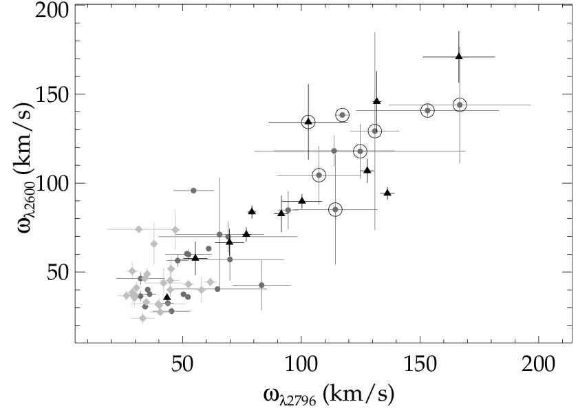
In fact all but one of the 8 systems in the FIRE sample (not just those in the lowest redshift bin) were classified as DLA/H i-rich systems based on their strong Fe ii absorption (=2.26 Å), but we have no measurements for any of these systems, and all of them have unusually large kinematic spreads (=128.3 km s-1). It may be that all of these are actually doubles, and the double class as a whole has evolved between lower redshifts and this epoch. Figure 20, which depicts the Mg ii and Fe ii kinematic spreads for all FIRE systems labeled as classic+C iv-deficient (light gray diamonds), DLA/H i-rich (dark gray circles), and doubles (black triangles), provides a case for re-classification: The large systems, depicted with open circles, occupy a region of space more heavily occupied by double systems. The square points on Figure 19 represent with the classifications of the systems changed to double.
V.2. Connection with DLAs
We showed in Section IV.1 that % of systems at high redshift (=3.402) are associated with DLAs. We can invert this question and consider what fraction of high redshift DLAs are associated with Mg ii systems. Prochaska et al. [50] provide measurements for the general DLA population at redshifts to 5.5, which are represented by the gray points in Figure 21. The black points represent of Mg ii-DLAs, calculated by multiplying total for Mg ii by the fraction of Mg ii systems exhibiting DLAs in each bin. For the lowest Mg ii-selected DLA redshift bin, we have no measurements so we simply used the fraction for the next highest bin. This is reasonably justified since the fraction of DLAs in this redshift bin (4/12) is very similar to the fraction for the representative subsample of Rao et al. [57] for (4/13). The highest Mg ii-selected bin has only one measurement (a DLA), and is therefore very uncertain.

This exercise suggests that all (or nearly all) DLAs have accompanying Mg ii absorption. This is to be expected since every observed DLA exhibits low-ionization metal line absorption in rest-frame UV [76, 36, 82, 35]. Moreover, Mg ii absorption has been found in every high redshift DLA for which it could have been observed [81]. These statements are also true for low redshift DLAs by construction, since most such DLAs were selected on the basis of strong Mg ii and Fe ii absorption [57]. This result informs our interpretation of Figure 16 depicting gas-phase metallicities for the Mg ii-selected (black) and H i-selected (light gray) absorption systems described in Section III.3.4. In particular, the Mg ii-selected metallicities for DLAs cannot be inconsistent with those of the general DLA population if these two groups are largely the same.
In the representative subsample at low redshifts () from Rao et al. [57] described in Section III.3.3, a smaller percentage of Mg ii systems correspond to DLAs (%), and these systems are more commonly associated with Lyman limit systems and/or sub-DLAs.
It is noteworthy that numerous papers have associated Mg ii systems—particularly the strong variety—with star formation and outflows (including in our Paper I), yet we find that this population overlaps very heavily with classical DLAs, which are generally not thought to result from outflows at all. Rather DLAs are often taken as building blocks of present day galaxies [82], either as the early progenitors of galactic disks [51] or merging baryonic clumps embedded in dark matter haloes [27, 48].
The connection between strong Mg ii absorption, winds [87, 59, e.g.,] and DLAs [56, e.g.,] is particularly interesting because low redshift galaxy-absorber studies see absorption systems in extended haloes out to kpc [15], while Mg ii-DLAs reside within kpc [72] of their respective hosts. If the strong Mg ii systems represent both winds and DLAs, then some fraction of the DLA population would reflect non-gravitational processes, and also the strong phase of Mg ii-absorbing wind evolution would only fill the halo region nearest to the stellar disk. This picture may be incomplete since both for the strong absorbers and empirically derived star formations rates fall from [12, 13] while the DLA linear density increases until at least [50, see Figure 21, or ]. This suggests that there may be some Mg ii-poor DLAs at ; although such systems have not been identified, it may be an interesting area for further study.
One possible alternative is to invoke two populations of strong absorbers: one corresponding to classical DLAs, and one associated with star formation driven winds. This theory is inspired by the taxonomic classifications of of Churchill et al. [18], and supported by Bond et al. [8], who explore the possibility that strong, double-troughed Mg ii absorbers trace winds. We see very faint evidence of evolution in our high redshift for the double systems that is consistent with this interpretation, but cannot be considered proof on account of the small number statistics.
V.3. Chemical Evolution
Figure 11 illustrates how the relative abundance of H i at fixed increases toward higher redshift while the heavy elements lines remain largely unchanged. One might interpret this as direct evidence of an increasing metallicity of Mg ii systems toward the present day. However this picture is complicated by uncertainties in the degree of saturation in the metal lines. At Å and above one expects some degree of saturation, particularly for systems with small or unresolved kinematic spreads. This effect could in principle mask a decrease in the metal column densities that tracks the observed change in from high to low redshifts.
We do estimate lower limits on the abundance directly for systems with measured H i, finding values consistent with the general DLA population, and even higher for lower , which correlates strongly with low . We also demonstrated that there exists a large overlap between the DLA and Mg ii population, and DLAs evolve in metallicity as a population, albeit weakly with a best-fit gradient of dex per unit redshift and large scatter [49].
The ratio is similar for weak and strong Mg ii systems (Figure 14), and evolves similarly in redshift for both these sets (Figure 15). The only discernible difference in metal line absorption between weak and strong Mg ii absorbers is a relative suppression of high ionization lines (Si iv, C iv) in the strong systems. This may be a straightforward result of ionization effects: the strong Mg ii are more likely to be associated with neutral DLAs, which are comparatively high in singly ionized species.
The similar and high metallicities we measure for the weaker Mg ii systems are difficult to reconcile with a scenario where these systems represent accretion of metal-poor gas from the IGM. These systems are at least as metal rich as the strong Mg ii and possibly even more so. However it could follow naturally if the Å absorbers represent the remnants of previously ejected material, possibly re-accreting as in a galactic fountain.
In this case the very flat evolution in is somewhat surprising in the absence of fallback, since the cumulative deposition of winds into the circumgalactic environment should in time increase the Mg ii cross section and hence incidence rate or characteristic abundance. At the Hubble time is just long enough to permit galaxy formation, wind propagation, and fallback for a few generations. It will be interesting to test this at as Mg ii re-emerges from the gap between the and bands. As one approaches the timescales for outflow and fallback become challenging, and in this scenario one would expect the Mg ii incidence rate to drop substantially.
VI. Conclusion
We have presented a large study of chemical abundance properties for the Mg ii systems detected with FIRE in Paper I. We employ optical spectra from MagE, MIKE, HIRES and SDSS to measure vacuum ultraviolet lines such as H i and C iv, as well as singly ionized states of carbon, silicon, iron, and aluminum. By combining these observations with carefully constructed low-redshift control samples, we perform a longitudinal study of H i and metals in Mg ii-selected systems from , a period of Gyr. Our main findings are as follows:
- 1.
The most significant difference in chemical evolution comes from H i, with higher redshift systems associated with much stronger H i column densities. A K-S test provided only a 0.008% probability that the low (, =0.927) and high (, =3.402) samples were drawn from the same distribution. At high redshifts, the fraction of systems associated with DLAs (%) is much larger than at lower redshifts (%). All high redshift Mg ii absorbers are associated with either DLAs or sub-DLAs.
- 2.
Comparison between for Mg ii-selected DLAs and the general DLA population at shows that a large fraction (if not all) of high redshift DLAs have absorption. The metallicities for both populations are not inconsistent with the hypothesis that the two groups are one and the same.
- 3.
Mg ii systems associated with sub-DLAs at high redshifts are quite metal rich, with some systems possessing lower limits greater than one-tenth solar in iron, silicon, and aluminum.
- 4.
Besides H i and Mg i, there is no evidence for strong chemical evolution in redshift for Mg ii-selected systems. The best candidates for moderate chemical evolution are among the high ionization states (Si iv 1393, Al iii 1854, and C iv 1548,1550) with stronger absorption at lower redshifts (plausibly from less H i shielding), but it is unclear that this evolution is not the result of small number counts.
- 5.
Weak and strong systems have ratios that are similar in both distribution and redshift evolution. There is some evidence that strong absorbers are associated with weaker high ionization states (Si iv, Al iii, C iv), potentially from shielding caused by their higher H i column densities.
- 6.
Applying the taxonomy defined in Churchill et al. [18] to the FIRE systems, we find that an overwhelming majority of systems are classic+C iv-deficient systems (84.2%). The linear density of this class does not significantly evolve between . Strong systems divide into the DLA/H i-rich and double classes. The strong double rises between and 3 and then falls. The strong DLA/H i-rich falls from to 5; the full DLA/H i-rich remains essentially constant over this redshift range.
- 7.
The strongest Mg ii systems (; 8 in total) possess unusually strong Fe ii absorption and Mg ii kinematic spreads (no or measurements are available for these systems). These systems do not fall nicely into any of the five system classes defined in Churchill et al. [18]. It is unclear whether they represent DLA/H i-rich systems (as they were typically classified), double systems, or an entirely new class generated by physical mechanisms not prevalent at .
The FIRE QSO sample was assembled with the goal of maximizing the redshift pathlength at higher redshifts in order to provide better estimates in this range. While the sample accomplished this stated goal, the high QSO redshifts (typically ) also greatly increased the probability that the rest-frame UV and near UV transitions (e.g., H i 1215 and C iv 1548) of systems would rest blueward of the Lyman break limit of at least one higher redshift absorber. As a result, our lowest and measurements for this FIRE sample are and , respectively. In addition to targeting high redshift QSOs to add information on high redshift systems, a new QSO spectroscopic sample looking to improve upon this study should include more QSOs with to better establish the chemical compositions of Mg ii systems. It should be possible to use the SDSS DR7 sample to obtain a list of lower redshift QSOs with multiple strong H i systems in this redshift range to strategically observe QSOs with high probabilities of finding Mg ii systems. If the H i distribution of these indicators follow that of the general population, then this selection process should not bias the chemical evolution study.
References
- [1] Aldcroft, T. L., Bechtold, J., & Elvis, M. 1994, ApJS, 93, 1
- [2] Asplund, M., Grevesse, N., Sauval, A. J., & Scott, P. 2009, ARA&A, 47, 481
- [3] Bahcall, J. N., et al. 1993, ApJS, 87, 1
- [4] —. 1996, ApJ, 457, 19
- [5] Barthel, P. D., Tytler, D. R., & Thomson, B. 1990, A&AS, 82, 339
- [6] Bernstein, R., Shectman, S. A., Gunnels, S. M., Mochnacki, S., & Athey, A. E. 2003, in Society of Photo-Optical Instrumentation Engineers (SPIE) Conference Series, Vol. 4841, Society of Photo-Optical Instrumentation Engineers (SPIE) Conference Series, ed. M. Iye & A. F. M. Moorwood, 1694–1704
- [7] Bochanski, J. J., et al. 2009, PASP, 121, 1409
- [8] Bond, N. A., Churchill, C. W., Charlton, J. C., & Vogt, S. S. 2001, ApJ, 562, 641
- [9] Bordoloi, R., et al. 2011, ApJ, 743, 10
- [10] Bouché, N., Murphy, M. T., Péroux, C., Csabai, I., & Wild, V. 2006, MNRAS, 371, 495
- [11] Bouché, N., Murphy, M. T., Péroux, C., Davies, R., Eisenhauer, F., Förster Schreiber, N. M., & Tacconi, L. 2007, ApJ, 669, L5
- [12] Bouwens, R. J., et al. 2010, ApJ, 725, 1587
- [13] —. 2011, ApJ, 737, 90
- [14] Chelouche, D., & Bowen, D. V. 2010, ApJ, 722, 1821
- [15] Chen, H.-W., Helsby, J. E., Gauthier, J.-R., Shectman, S. A., Thompson, I. B., & Tinker, J. L. 2010a, ApJ, 714, 1521
- [16] Chen, H.-W., Wild, V., Tinker, J. L., Gauthier, J.-R., Helsby, J. E., Shectman, S. A., & Thompson, I. B. 2010b, ApJ, 724, L176
- [17] Churchill, C. W., Mellon, R. R., Charlton, J. C., Jannuzi, B. T., Kirhakos, S., Steidel, C. C., & Schneider, D. P. 2000a, ApJS, 130, 91
- [18] —. 2000b, ApJ, 543, 577
- [19] Churchill, C. W., Rigby, J. R., Charlton, J. C., & Vogt, S. S. 1999, ApJS, 120, 51
- [20] Cooksey, K. L., Kao, M. M., Simcoe, R. A., O’Meara, J. M., & Prochaska, J. X. 2012, ArXiv e-prints
- [21] Cushing, M. C., Vacca, W. D., & Rayner, J. T. 2004, PASP, 116, 362
- [22] Ellison, S. L. 2006, MNRAS, 368, 335
- [23] Ellison, S. L., Songaila, A., Schaye, J., & Pettini, M. 2000, AJ, 120, 1175
- [24] Feigelson, E. D., & Nelson, P. I. 1985, ApJ, 293, 192
- [25] Foltz, C. B., Weymann, R. J., Peterson, B. M., Sun, L., Malkan, M. A., & Chaffee, Jr., F. H. 1986, ApJ, 307, 504
- [26] Gauthier, J., Chen, H., & Tinker, J. L. 2009, ApJ, 702, 50
- [27] Haehnelt, M. G., Steinmetz, M., & Rauch, M. 1998, ApJ, 495, 647
- [28] Jannuzi, B. T., et al. 1998, ApJS, 118, 1
- [29] Kacprzak, G. G., & Churchill, C. W. 2011, ArXiv e-prints
- [30] Kacprzak, G. G., Churchill, C. W., Evans, J. L., Murphy, M. T., & Steidel, C. C. 2011, MNRAS, 416, 3118
- [31] Kundic, T., Hogg, D. W., Blandford, R. D., Cohen, J. G., Lubin, L. M., & Larkin, J. E. 1997, AJ, 114, 2276
- [32] Lanzetta, K. M., Turnshek, D. A., & Wolfe, A. M. 1987, ApJ, 322, 739
- [33] Lavalley, M., Isobe, T., & Feigelson, E. 1992, in Astronomical Society of the Pacific Conference Series, Vol. 25, Astronomical Data Analysis Software and Systems I, ed. D. M. Worrall, C. Biemesderfer, & J. Barnes, 245
- [34] Lovegrove, E., & Simcoe, R. A. 2011, ApJ, 740, 30
- [35] Lu, L., & Wolfe, A. M. 1994, AJ, 108, 44
- [36] Lu, L., Wolfe, A. M., Turnshek, D. A., & Lanzetta, K. M. 1993, ApJS, 84, 1
- [37] Lundgren, B. F., et al. 2009, ApJ, 698, 819
- [38] Marshall, J. L., et al. 2008, in Society of Photo-Optical Instrumentation Engineers (SPIE) Conference Series, Vol. 7014, Society of Photo-Optical Instrumentation Engineers (SPIE) Conference Series
- [39] Matejek, M. S., & Simcoe, R. A. 2012, ArXiv e-prints
- [40] Ménard, B., Wild, V., Nestor, D., Quider, A., Zibetti, S., Rao, S., & Turnshek, D. 2011, MNRAS, 417, 801
- [41] Nestor, D. B., Johnson, B. D., Wild, V., Ménard, B., Turnshek, D. A., Rao, S., & Pettini, M. 2011, MNRAS, 412, 1559
- [42] Nestor, D. B., Turnshek, D. A., & Rao, S. M. 2005, ApJ, 628, 637
- [43] Newman, P. R., et al. 2004, in Society of Photo-Optical Instrumentation Engineers (SPIE) Conference Series, Vol. 5492, Society of Photo-Optical Instrumentation Engineers (SPIE) Conference Series, ed. A. F. M. Moorwood & M. Iye, 533–544
- [44] Noterdaeme, P., Srianand, R., & Mohan, V. 2010, MNRAS, 403, 906
- [45] Péroux, C., Dessauges-Zavadsky, M., D’Odorico, S., Kim, T.-S., & McMahon, R. G. 2007, MNRAS, 382, 177
- [46] Petitjean, P., & Bergeron, J. 1990, A&A, 231, 309
- [47] —. 1994, A&A, 283, 759
- [48] Pontzen, A., et al. 2008, MNRAS, 390, 1349
- [49] Prochaska, J. X., Gawiser, E., Wolfe, A. M., Castro, S., & Djorgovski, S. G. 2003, ApJ, 595, L9
- [50] Prochaska, J. X., Herbert-Fort, S., & Wolfe, A. M. 2005, ApJ, 635, 123
- [51] Prochaska, J. X., & Wolfe, A. M. 1997, ApJ, 487, 73
- [52] —. 2009, ApJ, 696, 1543
- [53] Prochaska, J. X., Wolfe, A. M., Howk, J. C., Gawiser, E., Burles, S. M., & Cooke, J. 2007, ApJS, 171, 29
- [54] Prochter, G. E., Prochaska, J. X., , & Burles, S. M. 2006, The Astrophysical Journal, 639, 766
- [55] Quider, A. M., Nestor, D. B., Turnshek, D. A., Rao, S. M., Monier, E. M., Weyant, A. N., & Busche, J. R. 2011, AJ, 141, 137
- [56] Rao, S. M., & Turnshek, D. A. 2000, ApJS, 130, 1
- [57] Rao, S. M., Turnshek, D. A., & Nestor, D. B. 2006, ApJ, 636, 610
- [58] Robertson, J. G., & Shaver, P. A. 1983, MNRAS, 204, 69P
- [59] Rubin, K. H. R., Weiner, B. J., Koo, D. C., Martin, C. L., Prochaska, J. X., Coil, A. L., & Newman, J. A. 2010, ApJ, 719, 1503
- [60] Sargent, W. L. W., Boksenberg, A., & Young, P. 1982a, ApJ, 252, 54
- [61] Sargent, W. L. W., Steidel, C. C., & Boksenberg, A. 1988, ApJ, 334, 22
- [62] —. 1989, ApJS, 69, 703
- [63] Sargent, W. L. W., Young, P., & Schneider, D. P. 1982b, ApJ, 256, 374
- [64] Sargent, W. L. W., Young, P. J., Boksenberg, A., Carswell, R. F., & Whelan, J. A. J. 1979, ApJ, 230, 49
- [65] Savage, B. D., & Sembach, K. R. 1991, ApJ, 379, 245
- [66] Schneider, D. P., et al. 2010, AJ, 139, 2360
- [67] Sheinis, A. I., Bolte, M., Epps, H. W., Kibrick, R. I., Miller, J. S., Radovan, M. V., Bigelow, B. C., & Sutin, B. M. 2002, PASP, 114, 851
- [68] Simcoe, R. A. 2011, ApJ, 738, 159
- [69] Simcoe, R. A., et al. 2008, in Society of Photo-Optical Instrumentation Engineers (SPIE) Conference Series, Vol. 7014, Society of Photo-Optical Instrumentation Engineers (SPIE) Conference Series
- [70] Simcoe, R. A., et al. 2010, in Society of Photo-Optical Instrumentation Engineers (SPIE) Conference Series, Vol. 7735, Society of Photo-Optical Instrumentation Engineers (SPIE) Conference Series
- [71] Steidel, C. C. 1990, ApJS, 72, 1
- [72] Steidel, C. C. 1995, in QSO Absorption Lines, ed. G. Meylan, 139
- [73] Steidel, C. C., & Sargent, W. L. W. 1992, ApJS, 80, 1
- [74] Storrie-Lombardi, L. J., McMahon, R. G., Irwin, M. J., & Hazard, C. 1996, ApJ, 468, 121
- [75] Tinker, J. L., & Chen, H. 2010, ApJ, 709, 1
- [76] Turnshek, D. A., Wolfe, A. M., Lanzetta, K. M., Briggs, F. H., Cohen, R. D., Foltz, C. B., Smith, H. E., & Wilkes, B. J. 1989, ApJ, 344, 567
- [77] Tytler, D., Boksenberg, A., Sargent, W. L. W., Young, P., & Kunth, D. 1987, ApJS, 64, 667
- [78] Vogt, S. S., et al. 1994, in Society of Photo-Optical Instrumentation Engineers (SPIE) Conference Series, Vol. 2198, Society of Photo-Optical Instrumentation Engineers (SPIE) Conference Series, ed. D. L. Crawford & E. R. Craine, 362
- [79] Weiner, B. J., et al. 2009, ApJ, 692, 187
- [80] Weymann, R. J., Williams, R. E., Peterson, B. M., & Turnshek, D. A. 1979, ApJ, 234, 33
- [81] Wolfe, A. M., Gawiser, E., & Prochaska, J. X. 2005, ARA&A, 43, 861
- [82] Wolfe, A. M., Turnshek, D. A., Lanzetta, K. M., & Lu, L. 1993, ApJ, 404, 480
- [83] Wright, A. E., Morton, D. C., Peterson, B. A., & Jauncey, D. L. 1982, MNRAS, 199, 81
- [84] Young, P., Sargent, W. L. W., & Boksenberg, A. 1982a, ApJ, 252, 10
- [85] —. 1982b, ApJS, 48, 455
- [86] Young, P. J., Sargent, W. L. W., Boksenberg, A., Carswell, R. F., & Whelan, J. A. J. 1979, ApJ, 229, 891
- [87] Zibetti, S., Ménard, B., Nestor, D. B., Quider, A. M., Rao, S. M., & Turnshek, D. A. 2007, ApJ, 658, 161
Complimentary Optical Spectra
| Object | Instrument | RangeaaMinimum wavelength listed is Ly- emission wavelength of QSO. | SNRbbMedian signal-to-noise ratio redward of Ly- forest. | ||
|---|---|---|---|---|---|
| (s) | (Å) | pix-1 | |||
| Q000026 | 4.10 | MagE | 900 | 619710283 | 23.0 |
| BR00046224 | 4.51 | (none) | ….. | ….. | ….. |
| BR00163544 | 4.15 | (none) | ….. | ….. | ….. |
| SDSS0106+0048 | 4.45 | SDSS | 2700 | 66249219 | 11.0 |
| SDSS01130935 | 3.67 | SDSS | 3601 | 56749221 | 14.8 |
| SDSS01270045 | 4.08 | SDSS | 5706 | 61789221 | 16.9 |
| SDSS01400839 | 3.71 | MagE | 900 | 572910283 | 38.5 |
| SDSS0203+0012 | 5.85 | (none) | ….. | ….. | ….. |
| BR03054957 | 4.78 | MagE | 900 | 702610284 | 27.2 |
| BR03222928 | 4.62 | MagE | 900 | 683210274 | 25.4 |
| SDSS03320654 | 3.69 | SDSS | 2700 | 57069221 | 5.2 |
| BR03311622 | 4.32 | MagE | 900 | 646710283 | 21.8 |
| BR03533820 | 4.58 | MIKE | 1800 | 67839423 | 43.7 |
| BR04185723 | 4.37 | MIKE | 2400 | 65289423 | 32.4 |
| SDSS0818+1722 | 5.90 | (none) | ….. | ….. | ….. |
| SDSS0836+0054 | 5.82 | MagE | 900 | 829010274 | 11.9 |
| SDSS0949+0335 | 4.05 | SDSS | 5104 | 61399246 | 22.7 |
| SDSS1020+0922 | 3.64 | MagE | 900 | 564010285 | 25.2 |
| SDSS1030+0524 | 6.28 | (none) | ….. | ….. | ….. |
| SDSS1110+0244 | 4.12 | MagE | 900 | 622410286 | 21.0 |
| SDSS1305+0521 | 4.09 | SDSS | 4200 | 61879221 | 9.4 |
| SDSS1306+0356 | 5.99 | MagE | 900 | 849710285 | 3.7 |
| ULAS1319+0950 | 6.13 | MagE | 900 | 866710285 | 5.5 |
| SDSS1402+0146 | 4.16 | SDSS | 2702 | 62729221 | 13.6 |
| SDSS1408+0205 | 4.01 | SDSS | 2702 | 60909221 | 9.7 |
| SDSS1411+1217 | 5.93 | MagE | 1800 | 842410284 | 3.5 |
| Q1422+2309 | 3.65 | HIRES | 3000 | 56527306 | 40.8 |
| SDSS1433+0227 | 4.72 | SDSS | 3601 | 69559221 | 11.3 |
| CFQS15091749 | 6.12 | MagE | 1800 | 865510285 | 5.2 |
| SDSS1538+0855 | 3.55 | SDSS | 2400 | 55319221 | 30.1 |
| SDSS1616+0501 | 4.87 | SDSS | 2400 | 71389221 | 9.1 |
| SDSS1620+0020 | 4.09 | SDSS | 5400 | 61879261 | 5.3 |
| SDSS16210042 | 3.70 | SDSS | 5400 | 57139261 | 27.5 |
| SDSS21470838 | 4.59 | SDSS | 2900 | 67929221 | 12.3 |
| SDSS22280757 | 5.14 | SDSS | 9607 | 74669221 | 3.2 |
| SDSS2310+1855 | 6.04 | (none) | ….. | ….. | ….. |
| BR23463729 | 4.21 | (none) | ….. | ….. | ….. |
Absorption Properties for the FIRE Mg ii-Selected Sample: Mg Ions
| Index # | Sightline | aaUpper limits are 3. | Class | |||
|---|---|---|---|---|---|---|
| (Å) | (Å) | (Å) | ||||
| 1bbSuspected false positive. | Q000026 | 2.184 | 0.114 | ……. | ||
| 2 | Q000026 | 3.390 | DLA/H i -Rich | |||
| 3 | BR00046224 | 2.663 | 0.079 | ……. | ||
| 4 | BR00046224 | 2.908 | 0.133 | Classic+C iv-Deficient | ||
| 5 | BR00046224 | 2.959 | Classic+C iv-Deficient | |||
| 6 | BR00046224 | 3.203 | 0.081 | Classic+C iv-Deficient | ||
| 7 | BR00046224 | 3.694 | 1.030ccBlended line. | ……. | ||
| 8 | BR00046224 | 3.776 | … | DLA/H i -Rich | ||
| 9 | BR00163544 | 2.783 | 0.047 | Classic+C iv-Deficient | ||
| 10 | BR00163544 | 2.819 | DLA/H i -Rich | |||
| 11 | BR00163544 | 2.949 | 0.067 | ……. | ||
| 12 | BR00163544 | 3.757 | … | Double | ||
| 13 | SDSS0106+0048 | 3.729 | … | Double | ||
| 14bbSuspected false positive. | SDSS01130935 | 2.825 | 0.055 | ……. | ||
| 15 | SDSS01130935 | 3.544 | ……. | |||
| 16 | SDSS01130935 | 3.617 | 0.045 | Classic | ||
| 17 | SDSS01270045 | 2.588 | 0.129 | Double | ||
| 18 | SDSS01270045 | 2.945 | Double | |||
| 19 | SDSS01270045 | 3.168 | 0.032 | Classic | ||
| 20 | SDSS01270045 | 3.728 | 0.055 | DLA/H i -Rich | ||
| 21 | SDSS01400839 | 2.241 | 0.077 | Classic+C iv-Deficient | ||
| 22 | SDSS01400839 | 3.081 | Classic | |||
| 23 | SDSS01400839 | 3.212 | 0.040 | ……. | ||
| 24 | SDSS0203+0012 | 3.711 | 0.202 | Classic+C iv-Deficient | ||
| 25 | SDSS0203+0012 | 4.313 | 0.062 | Classic+C iv-Deficient | ||
| 26 | SDSS0203+0012 | 4.482 | Classic | |||
| 27 | SDSS0203+0012 | 4.978 | 0.114 | DLA/H i -Rich | ||
| 28 | BR03054957 | 2.502 | 0.033 | Classic+C iv-Deficient | ||
| 29 | BR03054957 | 2.629 | DLA/H i -Rich | |||
| 30 | BR03054957 | 3.354 | 0.032 | Classic+C iv-Deficient | ||
| 31 | BR03054957 | 3.591 | DLA/H i -Rich | |||
| 32 | BR03054957 | 4.466 | 0.057 | DLA/H i -Rich | ||
| 33 | BR03222928 | 2.229 | 0.056 | Classic+C iv-Deficient | ||
| 34 | SDSS03320654 | 3.061 | 0.133 | Classic+C iv-Deficient | ||
| 35 | BR03311622 | 2.295 | 0.137 | DLA/H i -Rich | ||
| 36 | BR03311622 | 2.593 | 0.086 | ……. | ||
| 37 | BR03311622 | 2.927 | … | Double | ||
| 38 | BR03311622 | 3.557 | DLA/H i -Rich | |||
| 39 | BR03533820 | 1.987 | DLA/H i -Rich | |||
| 40 | BR03533820 | 2.696 | 0.036 | Classic+C iv-Deficient | ||
| 41 | BR03533820 | 2.754 | DLA/H i -Rich | |||
| 42 | BR04185723 | 2.030 | 0.272 | DLA/H i -Rich | ||
| 43 | BR04185723 | 2.978 | 1.106 | DLA/H i -Rich | ||
| 44 | SDSS0818+1722 | 3.563 | 0.151 | Classic+C iv-Deficient | ||
| 45 | SDSS0818+1722 | 4.431 | 0.055 | Classic+C iv-Deficient | ||
| 46 | SDSS0818+1722 | 5.065 | 0.048 | Classic+C iv-Deficient | ||
| 47 | SDSS0836+0054 | 2.299 | … | Classic+C iv-Deficient | ||
| 48 | SDSS0836+0054 | 3.744 | … | Double | ||
| 49 | SDSS0949+0335 | 2.289 | DLA/H i -Rich | |||
| 50 | SDSS0949+0335 | 3.310 | DLA/H i -Rich | |||
| 51 | SDSS1020+0922 | 2.046 | 0.077 | Classic+C iv-Deficient | ||
| 52 | SDSS1020+0922 | 2.593 | DLA/H i -Rich | |||
| 53 | SDSS1020+0922 | 2.749 | 0.079 | C iv-Deficient | ||
| 54 | SDSS1020+0922 | 3.479 | 0.105 | ……. | ||
| 55 | SDSS1030+0524 | 2.188 | 0.115 | Classic+C iv-Deficient | ||
| 56 | SDSS1030+0524 | 2.780 | 0.282 | Double | ||
| 57 | SDSS1030+0524 | 4.583 | 0.118 | Double | ||
| 58 | SDSS1030+0524 | 4.948 | 0.056 | C iv-Deficient | ||
| 59 | SDSS1030+0524 | 5.130 | 0.031 | ……. | ||
| 60 | SDSS1110+0244 | 2.119 | DLA/H i -Rich |
Absorption Properties for the FIRE Mg ii-Selected Sample: Mg Ions (Continued)
| Index # | Sightline | aaUpper limits are 3. | Class | |||
|---|---|---|---|---|---|---|
| (Å) | (Å) | (Å) | ||||
| 61 | SDSS1110+0244 | 2.223 | 0.090 | ……. | ||
| 62 | SDSS1305+0521 | 2.302 | 0.321 | DLA/H i -Rich | ||
| 63 | SDSS1305+0521 | 2.753 | 0.115 | Classic+C iv-Deficient | ||
| 64 | SDSS1305+0521 | 3.235 | 0.118 | C iv-Deficient | ||
| 65 | SDSS1305+0521 | 3.680 | … | DLA/H i -Rich | ||
| 66 | SDSS1306+0356 | 2.533 | 0.126 | DLA/H i -Rich | ||
| 67 | SDSS1306+0356 | 3.490 | 0.229 | Classic+C iv-Deficient | ||
| 68 | SDSS1306+0356 | 4.615 | DLA/H i -Rich | |||
| 69 | SDSS1306+0356 | 4.865 | 0.256 | Double | ||
| 70 | SDSS1306+0356 | 4.882 | DLA/H i -Rich | |||
| 71 | ULAS1319+0950 | 4.569 | 0.104 | Classic+C iv-Deficient | ||
| 72 | SDSS1402+0146 | 3.277 | DLA/H i -Rich | |||
| 73 | SDSS1402+0146 | 3.454 | 0.076 | C iv-Deficient | ||
| 74 | SDSS1408+0205 | 1.982 | DLA/H i -Rich | |||
| 75 | SDSS1408+0205 | 1.991 | 0.224 | Classic+C iv-Deficient | ||
| 76 | SDSS1408+0205 | 2.462 | 0.129 | DLA/H i -Rich | ||
| 77 | SDSS1411+1217 | 2.237 | Classic+C iv-Deficient | |||
| 78 | SDSS1411+1217 | 3.477 | 0.168 | Classic+C iv-Deficient | ||
| 79 | SDSS1411+1217 | 4.929 | 0.096 | Double | ||
| 80 | SDSS1411+1217 | 5.055 | 0.034 | ……. | ||
| 81 | SDSS1411+1217 | 5.250 | 0.072 | Classic | ||
| 82 | SDSS1411+1217 | 5.332 | … | ……. | ||
| 83dd and values adjusted relative to Paper I. | Q1422+2309 | 3.540 | Classic | |||
| 84 | SDSS1433+0227 | 2.772 | 0.051 | Classic+C iv-Deficient | ||
| 85 | CFQS15091749 | 3.128 | 0.094 | Double | ||
| 86 | CFQS15091749 | 3.266 | 0.079 | Classic+C iv-Deficient | ||
| 87 | CFQS15091749 | 3.392 | DLA/H i -Rich | |||
| 88 | SDSS1538+0855 | 2.638 | 0.040 | ……. | ||
| 89 | SDSS1538+0855 | 3.498 | 0.028 | ……. | ||
| 90 | SDSS1616+0501 | 2.741 | 0.232 | Classic+C iv-Deficient | ||
| 91 | SDSS1616+0501 | 3.275 | 0.367 | Classic+C iv-Deficient | ||
| 92 | SDSS1616+0501 | 3.396 | DLA/H i -Rich | |||
| 93 | SDSS1616+0501 | 3.450 | 0.525 | Classic+C iv-Deficient | ||
| 94 | SDSS1616+0501 | 3.733 | … | DLA/H i -Rich | ||
| 95 | SDSS1620+0020 | 2.910 | 0.250 | Double | ||
| 96 | SDSS1620+0020 | 3.273 | 0.129 | Classic | ||
| 97 | SDSS1620+0020 | 3.620 | Double | |||
| 98 | SDSS1620+0020 | 3.752 | … | DLA/H i -Rich | ||
| 99 | SDSS16210042 | 2.678 | 0.037 | ……. | ||
| 100 | SDSS16210042 | 3.106 | Classic | |||
| 101 | SDSS21470838 | 2.286 | 0.220 | Classic+C iv-Deficient | ||
| 102 | SDSS22280757 | 3.175 | 0.151 | Classic+C iv-Deficient | ||
| 103 | SDSS2310+1855 | 2.243 | 0.090 | Double | ||
| 104 | SDSS2310+1855 | 2.351 | 0.072 | Classic+C iv-Deficient | ||
| 105 | SDSS2310+1855 | 2.643 | Classic+C iv-Deficient | |||
| 106 | SDSS2310+1855 | 3.300 | 0.046 | Classic+C iv-Deficient | ||
| 107 | BR23463729 | 2.830 | DLA/H i -Rich | |||
| 108 | BR23463729 | 2.923 | 0.131 | Classic+C iv-Deficient | ||
| 109 | BR23463729 | 3.619 | Classic+C iv-Deficient | |||
| 110 | BR23463729 | 3.692 | 0.089 | Classic+C iv-Deficient |
The Low Redshift Compilation SampleaaThis table is available in a machine-readable form in the online journal. A portion is shown here for guidance regarding its form and content.ggfootnotetext: FeII 1608.
| ID # | Sightline | bbUpper limits are 5. | bbUpper limits are 5. | bbUpper limits are 5. | bbUpper limits are 5. | Ref.ccREFERENCES.–(1) Sargent et al. [62]; (2) Churchill et al. [17]; (3) Churchill et al. [19]; (4) Jannuzi et al. [28]; (5) Steidel & Sargent [73]; (6) Sargent et al. [64]; (7) Lanzetta et al. [32]; (8) Sargent et al. [61]; (9) Barthel et al. [5]; (10) Steidel [71]; (11) Storrie-Lombardi et al. [74]; (12) Sargent et al. [60]; (13) Aldcroft et al. [1]; (14) Young et al. [85]; (15) Petitjean & Bergeron [47]; (16) Wright et al. [83]; (17) Petitjean & Bergeron [46]; (18) Young et al. [84]; (19) Tytler et al. [77]; (20) Foltz et al. [25]; (21) Robertson & Shaver [58]; (22) Bahcall et al. [4]; (23) Bahcall et al. [3]. | |||
|---|---|---|---|---|---|---|---|---|---|
| (Å) | (Å) | (Å) | (Å) | (Å) | |||||
| L1 | 0001+087 | 3.243 | 1.085 | ….. | ….. | ….. | 1 | ||
| L2 | 0001+087 | 3.243 | 1.416 | ….. | ….. | ….. | 1 | ||
| L3 | 0002+051 | 1.899 | 0.591 | ….. | ….. | ….. | 2,3 | ||
| L4 | 0002+051 | 1.900 | 0.851 | 2,4,5 | |||||
| L5 | 0002+051 | 1.900 | 0.956 | 2,3,4 | |||||
| L6 | 0002422 | 2.758 | 0.837 | ….. | ….. | ….. | 6,7 | ||
| L7 | 0002422 | 2.758 | 1.541 | ….. | ….. | 7 | |||
| L8 | 0004+171 | 2.890 | 0.807 | ….. | ….. | ….. | ….. | 1 | |
| L9 | 00090138 | 2.000 | 1.386 | ….. | ….. | ….. | 5 | ||
| L10 | 0013004 | 2.086 | 0.447 | ….. | ….. | ….. | ….. | 8 | |
| L11 | 0013004 | 2.086 | 1.967 | ….. | 5,8 | ||||
| L12 | 0013004 | 2.086 | 1.972 | ….. | ddBlended line. | 5,8 | |||
| L13 | 0014+813 | 3.377 | 1.111 | ….. | ….. | ….. | 1,8 | ||
| L14 | 0014+813 | 3.377 | 1.113 | ….. | ….. | ….. | 8 | ||
| L15 | 0017+154 | 2.014 | 1.364 | ….. | ….. | ….. | eeFeII 2382. | 9 | |
| L16 | 0017+154 | 2.014 | 1.626 | ….. | ….. | 9 | |||
| L17 | 0019+0107 | 2.134 | 1.828 | ….. | ….. | ….. | 5 | ||
| L18 | 0027+0149 | 2.350 | 1.266 | ….. | ….. | ….. | 5 | ||
| L19 | 0029+073 | 3.259 | 1.176 | ….. | ….. | ….. | ddBlended line. | 1 | |
| L20 | 0029+073 | 3.259 | 1.403 | ….. | ….. | ….. | 1 | ||
| …………………………………. | |||||||||
| L277 | 1836+511 | 2.827 | 0.756 | ….. | ….. | ….. | ….. | 1 | |
| L278 | 1836+511 | 2.827 | 0.818 | ….. | ….. | ….. | 1 | ||
| L279 | 1836+511 | 2.827 | 0.864 | ….. | ….. | ….. | 1 | ||
| L280 | 1836+511 | 2.827 | 1.126 | ….. | ….. | ….. | 1 | ||
| L281 | 1857+566 | 1.573 | 0.715 | ….. | ….. | ….. | eeFeII 2382. | 9 | |
| L282 | 1857+566 | 1.573 | 1.234 | ….. | ….. | ….. | 9 | ||
| L283 | 1901+3155 | 0.635 | 0.390 | ….. | ….. | ….. | ….. | 13 | |
| L284 | 2000330 | 3.777 | 1.454 | ….. | ….. | ….. | ddBlended line. | 10 | |
| L285 | 2003025 | 1.457 | 1.211 | ….. | ….. | 13 | |||
| L286 | 2038012 | 2.783 | 0.795 | ….. | ….. | ….. | 1 | ||
| L287 | 2044168 | 1.943 | 1.328 | ….. | ….. | ….. | ….. | 7 | |
| L288 | 2048+196 | 2.364 | 1.116 | ….. | ….. | ….. | 9 | ||
| L289 | 2048+312 | 3.185 | 1.348 | ….. | ….. | ….. | 1 | ||
| L290 | 2116358 | 2.341 | 1.996 | ….. | ….. | ….. | 7 | ||
| L291 | 2126158 | 3.275 | 2.022 | ….. | ….. | 7,15 | |||
| L292 | 2128123 | 0.501 | 0.430 | 2,4,17,19 | |||||
| L293 | 2145+067 | 0.990 | 0.790 | 2,5,17,23 | |||||
| L294 | 2149+212 | 1.536 | 0.911 | ….. | ….. | ….. | 9 | ||
| L295 | 2149+212 | 1.536 | 1.002 | ….. | ….. | ….. | 9 | ||
| L296 | 2206199 | 2.559 | 0.752 | ….. | ….. | ….. | 8 | ||
| L297 | 2206199 | 2.559 | 1.017 | ….. | ….. | ….. | 8 | ||
| L298 | 2212299 | 2.703 | 1.938 | ….. | ….. | 7,9 | |||
| L299 | 2222+051 | 2.326 | 1.605 | ….. | ….. | ….. | 9 | ||
| L300 | 2233+131 | 3.295 | 1.026 | ….. | ….. | ….. | 1 | ||
| L301 | 2233+136 | 3.209 | 1.096 | ….. | ….. | ….. | 1 | ||
| L302 | 22370607 | 4.558 | 1.672 | ….. | ….. | ….. | 11 | ||
| L303 | 2239386 | 3.511 | 1.033 | ….. | ….. | ….. | ….. | 10 | |
| L304 | 2248+192 | 1.793 | 1.270 | ….. | ….. | ….. | eeFeII 2382. | 9 | |
| L305 | 2251+243 | 2.328 | 1.090 | ….. | ….. | 9,13 | |||
| L306 | 2341235 | 2.822 | 1.076 | ….. | ….. | ….. | 1 | ||
| L307 | 2342+089 | 2.784 | 0.723 | ….. | ….. | ….. | ….. | 8 | |
| L308 | 2342+089 | 2.784 | 0.838 | ….. | ….. | ….. | 8 | ||
| L309 | 2342+089 | 2.784 | 0.949 | ….. | ….. | ….. | 8 | ||
| L310 | 2354+144 | 1.813 | 1.576 | ….. | ….. | ….. | 9 | ||
| L311 | 2359+003 | 2.896 | 1.024 | ….. | ….. | ….. | 1 | ||
| L312 | 2359+003 | 2.896 | 1.344 | ….. | ….. | ….. | 1 | ||
| L313 | 2359+068 | 3.234 | 0.896 | ….. | ….. | ….. | ….. | 1 | |
and Metallicity Measurements, FIRE sample
| Index # | Sightline | [Fe/H]aaFe ii. | [C/H]bbC ii. | [Si/H]ccSi ii. | [Al/H]ddAl ii. | [Mg/H]eeMg ii. | ||
|---|---|---|---|---|---|---|---|---|
| (log cm-2) | ||||||||
| 2 | Q000026 | 3.390 | ……… | |||||
| 13 | SDSS0106+0048 | 3.729 | ……… | |||||
| 15 | SDSS01130935 | 3.544 | ……… | ……… | ……… | ……… | ||
| 16 | SDSS01130935 | 3.617 | ……… | ……… | ||||
| 18 | SDSS01270045 | 2.945 | ……… | ……… | ||||
| 19 | SDSS01270045 | 3.168 | ……… | ……… | ……… | ……… | ||
| 20 | SDSS01270045 | 3.728 | ||||||
| 22 | SDSS01400839 | 3.081 | ……… | |||||
| 23 | SDSS01400839 | 3.212 | ……… | ……… | ||||
| 30 | BR03054957 | 3.354 | ……… | ……… | ……… | |||
| 31 | BR03054957 | 3.591 | ……… | ……… | ……… | |||
| 32 | BR03054957 | 4.466 | ||||||
| 34 | SDSS03320654 | 3.061 | ……… | ……… | ……… | |||
| 38 | BR03311622 | 3.557 | ……… | ……… | ||||
| 50 | SDSS0949+0335 | 3.310 | ……… | |||||
| 52 | SDSS1020+0922 | 2.593 | ……… | |||||
| 53 | SDSS1020+0922 | 2.749 | ……… | |||||
| 54 | SDSS1020+0922 | 3.479 | ……… | ……… | ||||
| 64 | SDSS1305+0521 | 3.235 | ……… | ……… | ……… | |||
| 65 | SDSS1305+0521 | 3.680 | ||||||
| 72 | SDSS1402+0146 | 3.277 | ……… | |||||
| 73 | SDSS1402+0146 | 3.454 | ……… | |||||
| 83ffFeII 2586. | Q1422+2309 | 3.540 | ……… | ……… | ||||
| 88 | SDSS1538+0855 | 2.638 | ……… | ……… | ||||
| 89 | SDSS1538+0855 | 3.498 | ……… | ……… | ……… | |||
| 91 | SDSS1616+0501 | 3.275 | ……… | ……… | ……… | ……… | ||
| 92 | SDSS1616+0501 | 3.396 | ……… | ……… | ……… | |||
| 93 | SDSS1616+0501 | 3.450 | ……… | ……… | ……… | |||
| 94 | SDSS1616+0501 | 3.733 | ……… | |||||
| 97 | SDSS1620+0020 | 3.620 | ……… | ……… | ……… | ……… | ||
| 98 | SDSS1620+0020 | 3.752 | ||||||
| 99 | SDSS16210042 | 2.678 | ……… | ……… | ……… | ……… | ||
| 100 | SDSS16210042 | 3.106 | ……… |
Absorption Properties for the FIRE Mg ii-Selected Sample: H i 1215 and O i 1302
| Index # | Sightline | aaUpper limits are 3. | ||
|---|---|---|---|---|
| (Å) | (Å) | |||
| 2 | Q000026 | 3.390 | … | |
| 13 | SDSS0106+0048 | 3.729 | … | |
| 15 | SDSS01130935 | 3.544 | 0.142 | |
| 16 | SDSS01130935 | 3.617 | 0.156 | |
| 18 | SDSS01270045 | 2.945 | … | |
| 19 | SDSS01270045 | 3.168 | … | |
| 20 | SDSS01270045 | 3.728 | … | |
| 22 | SDSS01400839 | 3.081 | … | |
| 23 | SDSS01400839 | 3.212 | … | |
| 30 | BR03054957 | 3.354 | … | |
| 31 | BR03054957 | 3.591 | … | |
| 32 | BR03054957 | 4.466 | 0.488bbBlended line. | |
| 34 | SDSS03320654 | 3.061 | … | |
| 38 | BR03311622 | 3.557 | … | |
| 50 | SDSS0949+0335 | 3.310 | … | |
| 52 | SDSS1020+0922 | 2.593 | … | |
| 53 | SDSS1020+0922 | 2.749 | … | |
| 54 | SDSS1020+0922 | 3.479 | 0.033 | |
| 64 | SDSS1305+0521 | 3.235 | … | |
| 65 | SDSS1305+0521 | 3.680 | … | |
| 72 | SDSS1402+0146 | 3.277 | … | |
| 73 | SDSS1402+0146 | 3.454 | … | |
| 83 | Q1422+2309 | 3.540 | ||
| 88 | SDSS1538+0855 | 2.638 | … | |
| 89 | SDSS1538+0855 | 3.498 | 0.103 | |
| 91 | SDSS1616+0501 | 3.275 | … | |
| 92 | SDSS1616+0501 | 3.396 | … | |
| 93 | SDSS1616+0501 | 3.450 | … | |
| 94 | SDSS1616+0501 | 3.733 | … | |
| 97 | SDSS1620+0020 | 3.620 | … | |
| 98 | SDSS1620+0020 | 3.752 | … | |
| 99 | SDSS16210042 | 2.678 | … | |
| 100 | SDSS16210042 | 3.106 | … |
Absorption Properties for the FIRE Mg ii-Selected Sample: Fe Ions
| Index # | Sightline | aaUpper limits are 3. | aaUpper limits are 3. | aaUpper limits are 3. | aaUpper limits are 3. | aaUpper limits are 3. | aaUpper limits are 3. | |
|---|---|---|---|---|---|---|---|---|
| (Å) | (Å) | (Å) | (Å) | (Å) | (Å) | |||
| 1bbSuspected false positive. | Q000026 | 2.184 | … | 0.056 | 0.056 | 0.052 | 0.471ccBlended line. | 0.106 |
| 2 | Q000026 | 3.390 | ||||||
| 3 | BR00046224 | 2.663 | … | 0.236 | 0.266 | 0.334 | 0.258 | 0.264 |
| 4 | BR00046224 | 2.908 | … | 0.241 | 0.277ccBlended line. | 0.199 | 0.118 | 0.131 |
| 5 | BR00046224 | 2.959 | … | 0.203 | 0.293ccBlended line. | |||
| 6 | BR00046224 | 3.203 | … | 0.099 | 0.588ccBlended line. | |||
| 7 | BR00046224 | 3.694 | … | 0.081 | 0.180ccBlended line. | 0.335 | 0.133 | 0.090 |
| 8 | BR00046224 | 3.776 | … | |||||
| 9 | BR00163544 | 2.783 | … | 0.143 | 0.102 | 0.114 | 0.077 | 0.093 |
| 10 | BR00163544 | 2.819 | … | |||||
| 11 | BR00163544 | 2.949 | … | 0.082 | 0.136 | … | 0.152 | 0.084 |
| 12 | BR00163544 | 3.757 | … | … | … | … | ||
| 13 | SDSS0106+0048 | 3.729 | 0.448 | 0.091 | ||||
| 14bbSuspected false positive. | SDSS01130935 | 2.825 | … | 0.087 | 0.152 | 0.181 | 0.100 | 0.091 |
| 15 | SDSS01130935 | 3.544 | 0.148 | 0.115 | 0.064 | 0.086 | 0.045 | 0.042 |
| 16 | SDSS01130935 | 3.617 | 0.135 | 0.040 | 0.068 | 0.065 | 0.062 | 0.111 |
| 17 | SDSS01270045 | 2.588 | … | 0.142 | ||||
| 18 | SDSS01270045 | 2.945 | … | 0.118 | 0.104 | |||
| 19 | SDSS01270045 | 3.168 | 0.130 | 0.052 | 0.057 | 0.051 | 0.036 | 0.039 |
| 20 | SDSS01270045 | 3.728 | 0.421 | 0.074 | ||||
| 21 | SDSS01400839 | 2.241 | … | … | ||||
| 22 | SDSS01400839 | 3.081 | 0.088 | |||||
| 23 | SDSS01400839 | 3.212 | 0.031 | 0.101 | 0.059 | 0.064 | 0.052 | 0.059 |
| 24 | SDSS0203+0012 | 3.711 | … | 0.309 | 0.303 | 0.398 | 0.215 | 0.186 |
| 25 | SDSS0203+0012 | 4.313 | … | 0.248 | … | … | ||
| 26 | SDSS0203+0012 | 4.482 | … | … | … | |||
| 27 | SDSS0203+0012 | 4.978 | … | … | … | … | ||
| 28 | BR03054957 | 2.502 | … | 0.084 | 0.078 | 0.726ccBlended line. | 0.046 | 0.074 |
| 29 | BR03054957 | 2.629 | … | … | … | |||
| 30 | BR03054957 | 3.354 | … | 0.033 | … | … | ||
| 31 | BR03054957 | 3.591 | ||||||
| 32 | BR03054957 | 4.466 | … | … | ||||
| 33 | BR03222928 | 2.229 | … | … | … | |||
| 34 | SDSS03320654 | 3.061 | 0.360 | 0.835 | 0.229 | 0.225 | 0.257 | |
| 35 | BR03311622 | 2.295 | … | |||||
| 36 | BR03311622 | 2.593 | … | 0.075 | 0.154 | 0.094 | 0.098 | 0.183 |
| 37 | BR03311622 | 2.927 | … | 0.339ccBlended line. | 0.170 | 0.105 | ||
| 38 | BR03311622 | 3.557 | ||||||
| 39 | BR03533820 | 1.987 | … | |||||
| 40 | BR03533820 | 2.696 | … | 0.050 | 0.070 | 1.238ccBlended line. | 0.047 | 0.044 |
| 41 | BR03533820 | 2.754 | … | |||||
| 42 | BR04185723 | 2.030 | … | 0.291ccBlended line. | ||||
| 43 | BR04185723 | 2.978 | … | 0.374 | ||||
| 44 | SDSS0818+1722 | 3.563 | … | 0.178 | ||||
| 45 | SDSS0818+1722 | 4.431 | 0.029 | 0.089 | 0.041 | 0.062 | … | … |
| 46 | SDSS0818+1722 | 5.065 | 0.045 | … | … | … | ||
| 47 | SDSS0836+0054 | 2.299 | … | … | … | … | 0.149 | 0.081ccBlended line. |
| 48 | SDSS0836+0054 | 3.744 | … | 0.062 | … | … | ||
| 49 | SDSS0949+0335 | 2.289 | … | |||||
| 50 | SDSS0949+0335 | 3.310 | ||||||
| 51 | SDSS1020+0922 | 2.046 | … | 0.062 | 0.060 | |||
| 52 | SDSS1020+0922 | 2.593 | … | |||||
| 53 | SDSS1020+0922 | 2.749 | ||||||
| 54 | SDSS1020+0922 | 3.479 | … | 0.056 | 0.070 | 0.072 | … | 0.298 |
| 55 | SDSS1030+0524 | 2.188 | … | … | … | … | … | … |
| 56 | SDSS1030+0524 | 2.780 | … | 1.457ccBlended line. | 2.287ccBlended line. | 0.977ccBlended line. | 0.207 | |
| 57 | SDSS1030+0524 | 4.583 | … | … | ||||
| 58 | SDSS1030+0524 | 4.948 | … | … | … | … | 0.112 | |
| 59 | SDSS1030+0524 | 5.130 | 0.083 | … | … | … | 0.123 | 0.056 |
| 60 | SDSS1110+0244 | 2.119 | … |
Absorption Properties for the FIRE Mg ii-Selected Sample: Fe Ions (Continued)
| Index # | Sightline | aaUpper limits are 3. | aaUpper limits are 3. | aaUpper limits are 3. | aaUpper limits are 3. | aaUpper limits are 3. | aaUpper limits are 3. | |
|---|---|---|---|---|---|---|---|---|
| (Å) | (Å) | (Å) | (Å) | (Å) | (Å) | |||
| 61 | SDSS1110+0244 | 2.223 | … | 0.061 | … | … | 0.095 | 0.084 |
| 62 | SDSS1305+0521 | 2.302 | … | 0.389 | ||||
| 63 | SDSS1305+0521 | 2.753 | … | 0.311 | 0.123 | 0.116 | 0.093 | 0.141 |
| 64 | SDSS1305+0521 | 3.235 | 0.181 | 0.114 | 0.101 | 0.141 | ||
| 65 | SDSS1305+0521 | 3.680 | ||||||
| 66 | SDSS1306+0356 | 2.533 | … | … | … | … | ||
| 67 | SDSS1306+0356 | 3.490 | … | 0.104 | 0.110 | 0.139 | 0.101 | |
| 68 | SDSS1306+0356 | 4.615 | … | 0.097 | … | … | ||
| 69 | SDSS1306+0356 | 4.865 | … | … | … | … | ||
| 70 | SDSS1306+0356 | 4.882 | … | … | … | … | ||
| 71 | ULAS1319+0950 | 4.569 | 0.062 | 0.139 | 0.078 | … | … | |
| 72 | SDSS1402+0146 | 3.277 | 0.161 | |||||
| 73 | SDSS1402+0146 | 3.454 | 0.253ccBlended line. | 0.052 | 0.079 | … | … | |
| 74 | SDSS1408+0205 | 1.982 | … | 0.304 | ||||
| 75 | SDSS1408+0205 | 1.991 | … | 0.279 | 0.963ccBlended line. | 0.297 | 0.401 | 0.455 |
| 76 | SDSS1408+0205 | 2.462 | … | 0.506 | 0.466 | |||
| 77 | SDSS1411+1217 | 2.237 | … | … | … | … | … | … |
| 78 | SDSS1411+1217 | 3.477 | … | 0.375ccBlended line. | 0.234 | … | 0.115 | 0.107 |
| 79 | SDSS1411+1217 | 4.929 | 0.099 | … | … | … | 0.283 | |
| 80 | SDSS1411+1217 | 5.055 | 0.083 | … | … | … | 0.083 | 0.059 |
| 81 | SDSS1411+1217 | 5.250 | 0.052 | … | 0.461 | 0.296 | 0.033 | 0.045 |
| 82 | SDSS1411+1217 | 5.332 | 0.078 | 0.085 | 0.064 | 0.155 | 0.036 | 0.035 |
| 83 | Q1422+2309 | 3.540 | … | 0.028 | 0.019 | 0.017 | … | … |
| 84 | SDSS1433+0227 | 2.772 | … | |||||
| 85 | CFQS15091749 | 3.128 | … | 0.160 | 0.121 | |||
| 86 | CFQS15091749 | 3.266 | … | 0.139 | ||||
| 87 | CFQS15091749 | 3.392 | … | |||||
| 88 | SDSS1538+0855 | 2.638 | 0.155 | 0.106 | 0.057 | … | … | |
| 89 | SDSS1538+0855 | 3.498 | 0.073 | 0.040 | 0.047 | 0.046 | … | … |
| 90 | SDSS1616+0501 | 2.741 | … | 0.241 | 0.282 | |||
| 91 | SDSS1616+0501 | 3.275 | … | 0.236 | 0.254 | 0.218 | 0.170 | 0.195 |
| 92 | SDSS1616+0501 | 3.396 | … | |||||
| 93 | SDSS1616+0501 | 3.450 | 0.148 | 0.120 | 0.205 | 0.193 | 0.168 | |
| 94 | SDSS1616+0501 | 3.733 | 0.547 | 0.245 | 0.214 | 0.170 | 0.449ccBlended line. | |
| 95 | SDSS1620+0020 | 2.910 | … | 0.402 | 0.238 | 0.172 | ||
| 96 | SDSS1620+0020 | 3.273 | 0.343 | 0.217 | 0.187 | |||
| 97 | SDSS1620+0020 | 3.620 | 0.507 | 0.195 | 0.205 | 0.209 | 0.894ccBlended line. | 0.092 |
| 98 | SDSS1620+0020 | 3.752 | 0.874 | 0.207 | ||||
| 99 | SDSS16210042 | 2.678 | 0.086 | 0.070 | 0.065 | 0.079 | … | … |
| 100 | SDSS16210042 | 3.106 | 0.090 | |||||
| 101 | SDSS21470838 | 2.286 | … | 0.211 | 0.198 | 0.226 | 0.157 | |
| 102 | SDSS22280757 | 3.175 | … | 0.294 | 0.267 | 0.489 | 0.209 | 0.276 |
| 103 | SDSS2310+1855 | 2.243 | … | … | … | … | … | … |
| 104 | SDSS2310+1855 | 2.351 | … | … | … | … | ||
| 105 | SDSS2310+1855 | 2.643 | … | … | … | … | 0.162 | |
| 106 | SDSS2310+1855 | 3.300 | … | 0.061 | 0.302ccBlended line. | … | 0.059 | 0.060 |
| 107 | BR23463729 | 2.830 | … | 0.213 | ||||
| 108 | BR23463729 | 2.923 | … | 0.182 | 0.159 | 0.211 | 0.114 | |
| 109 | BR23463729 | 3.619 | … | … | 0.475ccBlended line. | 0.049ccBlended line. | 0.066 | 0.124 |
| 110 | BR23463729 | 3.692 | … | 0.530ccBlended line. | 0.612 | 0.138 |
Absorption Properties for the FIRE Mg ii-Selected Sample: Si Ions
| Index # | Sightline | aaUpper limits are 3. | aaUpper limits are 3. | aaUpper limits are 3. | aaUpper limits are 3. | aaUpper limits are 3. | ||
|---|---|---|---|---|---|---|---|---|
| (Å) | (Å) | (Å) | (Å) | (Å) | (Å) | |||
| 2 | Q000026 | 3.390 | … | … | … | … | ||
| 7 | BR00046224 | 3.694 | … | … | … | … | … | 0.176 |
| 8 | BR00046224 | 3.776 | … | … | … | … | … | 0.162 |
| 12 | BR00163544 | 3.757 | … | … | … | … | … | 0.079 |
| 13 | SDSS0106+0048 | 3.729 | … | … | … | … | 0.080 | |
| 14bbSuspected false positive. | SDSS01130935 | 2.825 | … | … | … | … | 0.173 | 0.161 |
| 15 | SDSS01130935 | 3.544 | 0.300ccBlended line. | 0.136 | 0.134 | 0.204 | ||
| 16 | SDSS01130935 | 3.617 | 0.164 | 0.200ccBlended line. | 0.112 | |||
| 17 | SDSS01270045 | 2.588 | … | … | … | … | … | 0.340ccBlended line. |
| 18 | SDSS01270045 | 2.945 | … | … | … | … | … | 0.129 |
| 19 | SDSS01270045 | 3.168 | … | … | … | … | … | 0.172 |
| 20 | SDSS01270045 | 3.728 | … | … | 0.603ccBlended line. | 0.120 | 0.104ccBlended line. | |
| 21 | SDSS01400839 | 2.241 | … | … | … | … | … | |
| 22 | SDSS01400839 | 3.081 | … | … | … | … | 0.035 | |
| 23 | SDSS01400839 | 3.212 | … | … | … | |||
| 27 | SDSS0203+0012 | 4.978 | … | … | … | … | … | 0.115 |
| 30 | BR03054957 | 3.354 | … | … | … | … | … | 0.035 |
| 32 | BR03054957 | 4.466 | … | … | 0.854ccBlended line. | 0.030 | ||
| 34 | SDSS03320654 | 3.061 | … | … | … | … | 0.468 | 0.798 |
| 37 | BR03311622 | 2.927 | … | … | … | … | … | 0.047 |
| 38 | BR03311622 | 3.557 | … | … | … | … | 0.170ccBlended line. | |
| 41 | BR03533820 | 2.754 | … | … | … | … | … | |
| 43 | BR04185723 | 2.978 | … | … | … | … | … | 0.233ccBlended line. |
| 45 | SDSS0818+1722 | 4.431 | … | … | … | … | … | 0.078 |
| 46 | SDSS0818+1722 | 5.065 | … | … | … | … | 0.033 | |
| 48 | SDSS0836+0054 | 3.744 | … | … | … | … | … | 0.053ccBlended line. |
| 50 | SDSS0949+0335 | 3.310 | … | … | … | … | 0.161 | |
| 52 | SDSS1020+0922 | 2.593 | … | … | … | … | … | |
| 53 | SDSS1020+0922 | 2.749 | … | … | … | … | 0.156ccBlended line. | |
| 54 | SDSS1020+0922 | 3.479 | … | 0.036 | 0.028 | 0.060 | ||
| 57 | SDSS1030+0524 | 4.583 | … | … | … | … | … | 0.049 |
| 58 | SDSS1030+0524 | 4.948 | … | … | … | … | 0.115 | |
| 59 | SDSS1030+0524 | 5.130 | … | … | … | … | 0.131 | 0.070 |
| 63 | SDSS1305+0521 | 2.753 | … | … | … | … | … | 0.373 |
| 64 | SDSS1305+0521 | 3.235 | … | … | … | … | 0.262 | 0.365 |
| 65 | SDSS1305+0521 | 3.680 | … | … | 0.221 | 0.277 | 0.193 | |
| 68 | SDSS1306+0356 | 4.615 | … | … | … | … | 0.100 | |
| 69 | SDSS1306+0356 | 4.865 | … | … | … | … | 0.106 | |
| 70 | SDSS1306+0356 | 4.882 | … | … | … | … | 0.099 | |
| 71 | ULAS1319+0950 | 4.569 | … | … | … | … | … | 0.073 |
| 72 | SDSS1402+0146 | 3.277 | … | … | … | … | 0.407 | |
| 73 | SDSS1402+0146 | 3.454 | … | … | … | … | 0.373 | |
| 76 | SDSS1408+0205 | 2.462 | … | … | … | … | … | 0.374 |
| 79 | SDSS1411+1217 | 4.929 | … | … | … | … | 0.344ccBlended line. | … |
| 80 | SDSS1411+1217 | 5.055 | … | … | 0.054 | 0.059 | 0.074 | |
| 81 | SDSS1411+1217 | 5.250 | … | … | 0.080 | 0.143 | ||
| 82 | SDSS1411+1217 | 5.332 | … | … | 0.051 | 0.130 | ||
| 83 | Q1422+2309 | 3.540 | 0.144ccBlended line. | … | ||||
| 88 | SDSS1538+0855 | 2.638 | … | … | … | … | 0.078 | |
| 89 | SDSS1538+0855 | 3.498 | 0.101 | 0.062 | 0.066 | 0.084 | 0.110 | |
| 91 | SDSS1616+0501 | 3.275 | … | … | … | … | … | 0.320 |
| 92 | SDSS1616+0501 | 3.396 | … | … | … | … | … | 0.415 |
| 93 | SDSS1616+0501 | 3.450 | … | … | … | … | … | 0.281 |
| 94 | SDSS1616+0501 | 3.733 | … | … | … | … | … | |
| 96 | SDSS1620+0020 | 3.273 | … | … | … | … | 0.325 | … |
| 97 | SDSS1620+0020 | 3.620 | … | … | … | … | ||
| 98 | SDSS1620+0020 | 3.752 | … | … | 1.507ccBlended line. | 0.195 | 0.215 | |
| 99 | SDSS16210042 | 2.678 | … | … | … | … | … | 0.113 |
| 100 | SDSS16210042 | 3.106 | … | … | 0.145 | |||
| 102 | SDSS22280757 | 3.175 | … | … | … | … | … | 0.375 |
| 110 | BR23463729 | 3.692 | … | … | … | … | … | 0.109 |
Absorption Properties for the FIRE Mg ii-Selected Sample: C and Al Ions
| Index # | Sightline | aaUpper limits are 3. | aaUpper limits are 3. | aaUpper limits are 3. | aaUpper limits are 3. | aaUpper limits are 3. | aaUpper limits are 3. | |
|---|---|---|---|---|---|---|---|---|
| (Å) | (Å) | (Å) | (Å) | (Å) | (Å) | |||
| 2 | Q000026 | 3.390 | … | |||||
| 7 | BR00046224 | 3.694 | … | … | … | … | 0.205 | 0.238 |
| 8 | BR00046224 | 3.776 | … | … | … | … | 0.208 | 0.201 |
| 12 | BR00163544 | 3.757 | … | … | … | … | 0.111 | 0.096 |
| 13 | SDSS0106+0048 | 3.729 | … | 0.080 | ||||
| 14bbSuspected false positive. | SDSS01130935 | 2.825 | … | 0.161 | 0.165 | 0.170 | 0.143 | 0.152 |
| 15 | SDSS01130935 | 3.544 | 0.123 | 0.181 | 0.063 | 0.079 | ||
| 16 | SDSS01130935 | 3.617 | 0.370 | 0.095 | 0.075 | |||
| 17 | SDSS01270045 | 2.588 | … | … | … | … | 0.169 | |
| 18 | SDSS01270045 | 2.945 | … | … | … | 0.472ccBlended line. | 0.236 | |
| 19 | SDSS01270045 | 3.168 | … | 0.144 | 0.140 | 0.160 | ||
| 20 | SDSS01270045 | 3.728 | 0.197 | 0.066 | 0.075 | |||
| 21 | SDSS01400839 | 2.241 | … | … | … | … | 0.429ccBlended line. | |
| 22 | SDSS01400839 | 3.081 | … | … | ||||
| 23 | SDSS01400839 | 3.212 | … | 0.026 | 0.026 | 0.031 | ||
| 26 | SDSS0203+0012 | 4.482 | … | 0.802 | … | 0.308 | 0.493 | |
| 27 | SDSS0203+0012 | 4.978 | … | 0.333 | 0.308 | 0.351 | 0.279 | |
| 30 | BR03054957 | 3.354 | … | … | … | … | 1.744ccBlended line. | 0.046 |
| 31 | BR03054957 | 3.591 | … | 0.582ccBlended line. | 1.021ccBlended line. | 0.056 | 0.057 | |
| 32 | BR03054957 | 4.466 | 0.042 | |||||
| 34 | SDSS03320654 | 3.061 | … | 0.599 | 1.214 | 0.985 | 0.803 | 0.808 |
| 36 | BR03311622 | 2.593 | … | … | … | … | 0.020 | |
| 37 | BR03311622 | 2.927 | … | … | … | |||
| 38 | BR03311622 | 3.557 | … | … | 0.086 | 0.105 | ||
| 41 | BR03533820 | 2.754 | … | … | … | … | ||
| 43 | BR04185723 | 2.978 | … | … | … | … | ||
| 45 | SDSS0818+1722 | 4.431 | … | … | … | 0.048 | 0.049 | |
| 46 | SDSS0818+1722 | 5.065 | … | … | … | … | … | |
| 48 | SDSS0836+0054 | 3.744 | … | … | … | … | 0.500ccBlended line. | |
| 50 | SDSS0949+0335 | 3.310 | … | 0.243 | 0.247 | |||
| 51 | SDSS1020+0922 | 2.046 | … | … | … | … | … | |
| 52 | SDSS1020+0922 | 2.593 | … | … | … | 0.041 | ||
| 53 | SDSS1020+0922 | 2.749 | … | 0.039 | 0.039 | |||
| 54 | SDSS1020+0922 | 3.479 | 0.086 | 0.080 | ||||
| 57 | SDSS1030+0524 | 4.583 | … | … | … | 0.105 | 0.101 | |
| 58 | SDSS1030+0524 | 4.948 | … | 0.086 | 0.065 | |||
| 59 | SDSS1030+0524 | 5.130 | … | 0.215 | 0.051 | … | … | |
| 63 | SDSS1305+0521 | 2.753 | … | … | … | 0.135 | 0.267 | 0.368 |
| 64 | SDSS1305+0521 | 3.235 | … | 0.262 | 0.234 | 0.311 | 2.125 | 2.063ccBlended line. |
| 65 | SDSS1305+0521 | 3.680 | 0.411 | 0.281 | 0.205 | 0.203 | ||
| 68 | SDSS1306+0356 | 4.615 | … | 0.146 | 0.064 | 0.065 | ||
| 69 | SDSS1306+0356 | 4.865 | … | 0.121 | ||||
| 70 | SDSS1306+0356 | 4.882 | … | 0.038 | 0.054 | |||
| 71 | ULAS1319+0950 | 4.569 | … | … | … | 0.076 | 0.166 | |
| 72 | SDSS1402+0146 | 3.277 | … | 0.158 | 0.170 | 0.225 | 0.312 | |
| 73 | SDSS1402+0146 | 3.454 | … | 0.180 | 0.143 | 0.258 | 0.459 | |
| 76 | SDSS1408+0205 | 2.462 | … | … | … | … | 0.251 | 0.221 |
| 79 | SDSS1411+1217 | 4.929 | … | … | … | |||
| 80 | SDSS1411+1217 | 5.055 | … | … | … | 0.055 | 0.055 | 0.087 |
| 81 | SDSS1411+1217 | 5.250 | … | 0.240 | 0.077 | |||
| 82 | SDSS1411+1217 | 5.332 | 0.121 | 0.112 | 0.033 | 0.054 | 0.046 | |
| 83 | Q1422+2309 | 3.540 | … | 0.029 | 0.030 | |||
| 84 | SDSS1433+0227 | 2.772 | … | … | … | … | ||
| 88 | SDSS1538+0855 | 2.638 | … | 0.070 | 0.081 | 0.082 | ||
| 89 | SDSS1538+0855 | 3.498 | … | 0.070 | 0.071 | 0.050 | 0.052 | |
| 91 | SDSS1616+0501 | 3.275 | … | … | … | … | 0.312 | 0.437 |
| 92 | SDSS1616+0501 | 3.396 | … | … | … | 1.147ccBlended line. | 0.286 | |
| 93 | SDSS1616+0501 | 3.450 | … | … | … | 0.244 | 0.270 | 0.474 |
| 94 | SDSS1616+0501 | 3.733 | … | 0.247 | 0.248 | 0.225 | ||
| 95 | SDSS1620+0020 | 2.910 | … | … | … | 0.454 | 0.580ccBlended line. | 1.846 |
| 96 | SDSS1620+0020 | 3.273 | … | … | 0.321 | 0.455 | ||
| 97 | SDSS1620+0020 | 3.620 | … | … | ||||
| 98 | SDSS1620+0020 | 3.752 | 0.523 | 0.712 | 0.294 | 0.301 | ||
| 99 | SDSS16210042 | 2.678 | … | … | … | 0.070 | 0.081 | 0.078 |
| 100 | SDSS16210042 | 3.106 | … | 0.191 | ||||
| 102 | SDSS22280757 | 3.175 | … | … | … | … | 0.562 | 0.741 |
| 109 | BR23463729 | 3.619 | … | … | … | … | 0.136 | 0.118 |
| 110 | BR23463729 | 3.692 | … | … | … | … | 0.089 | 0.108 |
Kinematic Properties, FIRE sample
| Index | Sightline | |||||||
|---|---|---|---|---|---|---|---|---|
| (km s-1) | (km s-1) | (km s-1) | (km s-1) | (km s-1) | (km s-1) | |||
| 1aaSuspected false positive. | Q000026 | 2.184 | ….. | ….. | ….. | ….. | ||
| 2 | Q000026 | 3.390 | ||||||
| 3 | BR00046224 | 2.663 | ….. | ….. | ….. | ….. | ||
| 4 | BR00046224 | 2.908 | ….. | ….. | ….. | ….. | ||
| 5 | BR00046224 | 2.959 | ….. | ….. | ||||
| 6 | BR00046224 | 3.203 | bbFeII 2586. | bbFeII 2586. | ….. | ….. | ||
| 7 | BR00046224 | 3.694 | ….. | ….. | ….. | ….. | ||
| 8 | BR00046224 | 3.776 | ccMgII 2803. | ….. | ….. | |||
| 9 | BR00163544 | 2.783 | ….. | ….. | ….. | ….. | ||
| 10 | BR00163544 | 2.819 | ….. | ….. | ||||
| 11 | BR00163544 | 2.949 | ….. | ….. | ….. | ….. | ||
| 12 | BR00163544 | 3.757 | ….. | ….. | ||||
| 13 | SDSS0106+0048 | 3.729 | ….. | ….. | ||||
| 14aaSuspected false positive. | SDSS01130935 | 2.825 | ….. | ….. | ….. | ….. | ||
| 15 | SDSS01130935 | 3.544 | ….. | ….. | ….. | ….. | ||
| 16 | SDSS01130935 | 3.617 | ….. | ….. | ….. | ….. | ||
| 17 | SDSS01270045 | 2.588 | ….. | ….. | ||||
| 18 | SDSS01270045 | 2.945 | ….. | ….. | ||||
| 19 | SDSS01270045 | 3.168 | ….. | ….. | ….. | ….. | ||
| 20 | SDSS01270045 | 3.728 | ….. | ….. | ||||
| 21 | SDSS01400839 | 2.241 | ….. | ….. | ||||
| 22 | SDSS01400839 | 3.081 | ||||||
| 23 | SDSS01400839 | 3.212 | ….. | ….. | ….. | ….. | ||
| 24 | SDSS0203+0012 | 3.711 | ….. | ….. | ….. | ….. | ||
| 25 | SDSS0203+0012 | 4.313 | ddFeII 2382. | ddFeII 2382. | ….. | ….. | ||
| 26 | SDSS0203+0012 | 4.482 | ddFeII 2382. | ddFeII 2382. | ….. | |||
| 27 | SDSS0203+0012 | 4.978 | bbFeII 2586. | ….. | ….. | |||
| 28 | BR03054957 | 2.502 | ….. | ….. | ….. | ….. | ||
| 29 | BR03054957 | 2.629 | ddFeII 2382. | ddFeII 2382. | ….. | ….. | ||
| 30 | BR03054957 | 3.354 | ddFeII 2382. | ddFeII 2382. | ….. | ….. | ||
| 31 | BR03054957 | 3.591 | ||||||
| 32 | BR03054957 | 4.466 | ccMgII 2803. | ddFeII 2382. | ddFeII 2382. | |||
| 33 | BR03222928 | 2.229 | ….. | ….. | ||||
| 34 | SDSS03320654 | 3.061 | ddFeII 2382. | ddFeII 2382. | ….. | ….. | ||
| 35 | BR03311622 | 2.295 | ….. | ….. | ||||
| 36 | BR03311622 | 2.593 | ….. | ….. | ….. | ….. | ||
| 37 | BR03311622 | 2.927 | ….. | ….. | ||||
| 38 | BR03311622 | 3.557 | ||||||
| 39 | BR03533820 | 1.987 | ….. | ….. | ||||
| 40 | BR03533820 | 2.696 | ….. | ….. | ….. | ….. | ||
| 41 | BR03533820 | 2.754 | bbFeII 2586. | ….. | ….. | |||
| 42 | BR04185723 | 2.030 | ….. | ….. | ||||
| 43 | BR04185723 | 2.978 | ….. | ….. | ||||
| 44 | SDSS0818+1722 | 3.563 | ….. | ….. | ||||
| 45 | SDSS0818+1722 | 4.431 | ….. | ….. | ….. | ….. | ||
| 46 | SDSS0818+1722 | 5.065 | ….. | ….. | ||||
| 47 | SDSS0836+0054 | 2.299 | ….. | ….. | ….. | ….. | ||
| 48 | SDSS0836+0054 | 3.744 | ….. | ….. | ||||
| 49 | SDSS0949+0335 | 2.289 | bbFeII 2586. | ….. | ….. | |||
| 50 | SDSS0949+0335 | 3.310 | ….. | ….. | ||||
| 51 | SDSS1020+0922 | 2.046 | ….. | ….. | ||||
| 52 | SDSS1020+0922 | 2.593 | bbFeII 2586. | bbFeII 2586. | ….. | ….. | ||
| 53 | SDSS1020+0922 | 2.749 | ||||||
| 54 | SDSS1020+0922 | 3.479 | ….. | ….. | ||||
| 55 | SDSS1030+0524 | 2.188 | ….. | ….. | ….. | ….. | ||
| 56 | SDSS1030+0524 | 2.780 | ….. | ….. | ||||
| 57 | SDSS1030+0524 | 4.583 | ddFeII 2382. | ddFeII 2382. | ….. | ….. | ||
| 58 | SDSS1030+0524 | 4.948 | ||||||
| 59 | SDSS1030+0524 | 5.130 | ….. | ….. | ||||
| 60 | SDSS1110+0244 | 2.119 | ….. | ….. |
Kinematic Properties, FIRE sample (Continued)
| Index | Sightline | |||||||
|---|---|---|---|---|---|---|---|---|
| (km s-1) | (km s-1) | (km s-1) | (km s-1) | (km s-1) | (km s-1) | |||
| 61 | SDSS1110+0244 | 2.223 | ….. | ….. | ….. | ….. | ||
| 62 | SDSS1305+0521 | 2.302 | ….. | ….. | ….. | ….. | ||
| 63 | SDSS1305+0521 | 2.753 | ….. | ….. | ….. | ….. | ||
| 64 | SDSS1305+0521 | 3.235 | ddFeII 2382. | ddFeII 2382. | ….. | ….. | ||
| 65 | SDSS1305+0521 | 3.680 | ….. | ….. | ||||
| 66 | SDSS1306+0356 | 2.533 | ….. | ….. | ….. | |||
| 67 | SDSS1306+0356 | 3.490 | ddFeII 2382. | ddFeII 2382. | ….. | ….. | ||
| 68 | SDSS1306+0356 | 4.615 | ddFeII 2382. | ddFeII 2382. | ||||
| 69 | SDSS1306+0356 | 4.865 | ||||||
| 70 | SDSS1306+0356 | 4.882 | bbFeII 2586. | |||||
| 71 | ULAS1319+0950 | 4.569 | ddFeII 2382. | ddFeII 2382. | ….. | ….. | ||
| 72 | SDSS1402+0146 | 3.277 | ….. | ….. | ||||
| 73 | SDSS1402+0146 | 3.454 | eeFeII 2374. | eeFeII 2374. | ….. | ….. | ||
| 74 | SDSS1408+0205 | 1.982 | ….. | ….. | ….. | ….. | ||
| 75 | SDSS1408+0205 | 1.991 | ccMgII 2803. | ….. | ….. | ….. | ….. | |
| 76 | SDSS1408+0205 | 2.462 | ….. | ….. | ||||
| 77 | SDSS1411+1217 | 2.237 | ….. | ….. | ….. | ….. | ||
| 78 | SDSS1411+1217 | 3.477 | ….. | ….. | ….. | ….. | ||
| 79 | SDSS1411+1217 | 4.929 | ||||||
| 80 | SDSS1411+1217 | 5.055 | ….. | ….. | ….. | ….. | ||
| 81 | SDSS1411+1217 | 5.250 | ….. | ….. | ||||
| 82 | SDSS1411+1217 | 5.332 | ….. | ….. | ….. | ….. | ||
| 83 | Q1422+2309 | 3.540 | ….. | ….. | ||||
| 84 | SDSS1433+0227 | 2.772 | ….. | ….. | ||||
| 85 | CFQS15091749 | 3.128 | ….. | ….. | ||||
| 86 | CFQS15091749 | 3.266 | ….. | ….. | ||||
| 87 | CFQS15091749 | 3.392 | bbFeII 2586. | ….. | ….. | |||
| 88 | SDSS1538+0855 | 2.638 | ddFeII 2382. | ddFeII 2382. | ….. | ….. | ||
| 89 | SDSS1538+0855 | 3.498 | ….. | ….. | ….. | ….. | ||
| 90 | SDSS1616+0501 | 2.741 | ccMgII 2803. | bbFeII 2586. | bbFeII 2586. | ….. | ….. | |
| 91 | SDSS1616+0501 | 3.275 | ….. | ….. | ….. | ….. | ||
| 92 | SDSS1616+0501 | 3.396 | ccMgII 2803. | ….. | ….. | |||
| 93 | SDSS1616+0501 | 3.450 | ddFeII 2382. | ddFeII 2382. | ….. | ….. | ||
| 94 | SDSS1616+0501 | 3.733 | ccMgII 2803. | ff[O/H] = (O i). | ffFeII 2344. | ….. | ….. | |
| 95 | SDSS1620+0020 | 2.910 | ….. | ….. | ||||
| 96 | SDSS1620+0020 | 3.273 | ….. | ….. | ||||
| 97 | SDSS1620+0020 | 3.620 | ….. | ….. | ….. | ….. | ||
| 98 | SDSS1620+0020 | 3.752 | ….. | ….. | ||||
| 99 | SDSS16210042 | 2.678 | ….. | ….. | ….. | ….. | ||
| 100 | SDSS16210042 | 3.106 | ccMgII 2803. | ….. | ….. | |||
| 101 | SDSS21470838 | 2.286 | ….. | ….. | ||||
| 102 | SDSS22280757 | 3.175 | ….. | ….. | ….. | ….. | ||
| 103 | SDSS2310+1855 | 2.243 | ….. | ….. | ….. | ….. | ||
| 104 | SDSS2310+1855 | 2.351 | ….. | ….. | ||||
| 105 | SDSS2310+1855 | 2.643 | ….. | ….. | ||||
| 106 | SDSS2310+1855 | 3.300 | ….. | ….. | ….. | ….. | ||
| 107 | BR23463729 | 2.830 | ….. | ….. | ||||
| 108 | BR23463729 | 2.923 | ….. | ….. | ||||
| 109 | BR23463729 | 3.619 | ….. | ….. | ….. | ….. | ||
| 110 | BR23463729 | 3.692 | ….. | ….. |
Comparison Samples Statistics: Two Redshift Bins
| Ion | Detections | Upper LimitsaaUpper Limits are 5.bbValues in parentheses are upper limits derived from blended lines. | Min | Max | |
|---|---|---|---|---|---|
| (Å) | (Å) | ||||
| Low Redshift, | |||||
| HI 1215 | 0.864 | 18 | 2 (1) | ||
| MgII 2796 | 1.128 | 272 | 0 | ||
| MgI 2852 | 1.128 | 46 | 214 (5) | ||
| FeII 2374 | 1.215 | 36 | 137 (5) | ||
| FeII 2586 | 1.190 | 66 | 139 (3) | ||
| FeII 2600 | 1.173 | 94 | 122 (5) | ||
| CII 1334 | 1.211 | 23 | 9 (2) | ||
| CIV 1548 | 1.255 | 36 | 12 | ||
| CIV 1550 | 1.322 | 24 | 17 (5) | ||
| SiII 1526 | 1.276 | 17 | 20 | ||
| SiIV 1393 | 1.237 | 20 | 15 (2) | ||
| SiIV 1402 | 1.366 | 14 | 13 | ||
| AlII 1670 | 1.117 | 17 | 32 (2) | ||
| AlIII 1854 | 1.209 | 13 | 37 | ||
| High Redshift, | |||||
| HI 1215 | 3.402 | 27 | 0 | ||
| MgII 2796 | 3.184 | 97 | 0 | ||
| MgI 2852 | 3.174 | 13 | 73 | ||
| FeII 2374 | 3.123 | 22 | 59 (5) | ||
| FeII 2586 | 3.130 | 36 | 47 (2) | ||
| FeII 2600 | 3.147 | 49 | 32 (3) | ||
| CII 1334 | 3.360 | 8 | 0 | ||
| CIV 1548 | 3.647 | 24 | 8 | ||
| CIV 1550 | 3.647 | 19 | 13 (1) | ||
| SiII 1526 | 3.728 | 21 | 7 (2) | ||
| SiIV 1393 | 3.439 | 7 | 3 (2) | ||
| SiIV 1402 | 3.533 | 5 | 6 (1) | ||
| AlII 1670 | 3.693 | 18 | 20 (2) | ||
| AlIII 1854 | 3.438 | 7 | 49 (4) | ||
| SDSS, | |||||
| MgII 2796 | 1.064 | 1975 | 0 | ||
| MgI 2852 | 1.050 | 28 | 1900 | ||
| FeII 2374 | 1.128 | 37 | 1651 | ||
| FeII 2586 | 1.054 | 97 | 1747 | ||
| FeII 2600 | 1.078 | 216 | 1702 | ||
| CII 1334 | 1.921 | 5 | 6 | ||
| CIV 1548 | 1.622 | 127 | 208 | ||
| CIV 1550 | 1.615 | 87 | 169 | ||
| SiII 1526 | 1.712 | 20 | 47 | ||
| SiIV 1393 | 1.867 | 16 | 13 | ||
| SiIV 1402 | 1.861 | 6 | 14 | ||
| AlII 1670 | 1.430 | 42 | 346 | ||
| AlIII 1854 | 1.292 | 5 | 596 | ||
Comparison Samples Statistics: Three Redshift Bins
| Ion | Detections | Upper LimitsaaUpper Limits are 5.bbValues in parentheses are upper limits derived from blended lines. | Min | Max | |
|---|---|---|---|---|---|
| (Å) | (Å) | ||||
| Low Redshift, | |||||
| HI 1215 | 0.752 | 17 | 1 | ||
| MgII 2796 | 0.968 | 217 | 0 | ||
| MgI 2852 | 0.973 | 37 | 172 (3) | ||
| FeII 2374 | 1.008 | 26 | 101 (2) | ||
| FeII 2586 | 0.997 | 47 | 107 (3) | ||
| FeII 2600 | 0.985 | 67 | 97 (4) | ||
| CII 1334 | 0.736 | 12 | 6 | ||
| CIV 1548 | 0.857 | 17 | 10 | ||
| CIV 1550 | 0.887 | 12 | 9 | ||
| SiII 1526 | 0.883 | 9 | 12 | ||
| SiIV 1393 | 0.810 | 10 | 10 | ||
| SiIV 1402 | 0.875 | 6 | 7 | ||
| AlII 1670 | 0.834 | 12 | 22 (1) | ||
| AlIII 1854 | 0.883 | 5 | 27 | ||
| Mid Redshift, | |||||
| HI 1215 | 2.405 | 4 | 1 (1) | ||
| MgII 2796 | 2.092 | 100 | 0 | ||
| MgI 2852 | 2.091 | 16 | 76 (2) | ||
| FeII 2374 | 2.117 | 20 | 63 (6) | ||
| FeII 2586 | 2.098 | 35 | 56 (1) | ||
| FeII 2600 | 2.084 | 51 | 39 (2) | ||
| CII 1334 | 1.851 | 13 | 3 (2) | ||
| CIV 1548 | 1.839 | 22 | 3 | ||
| CIV 1550 | 1.852 | 14 | 10 (5) | ||
| SiII 1526 | 1.870 | 11 | 8 | ||
| SiIV 1393 | 1.834 | 12 | 5 (2) | ||
| SiIV 1402 | 1.851 | 9 | 7 | ||
| AlII 1670 | 2.059 | 11 | 12 (1) | ||
| AlIII 1854 | 2.148 | 13 | 21 (2) | ||
| High Redshift, | |||||
| HI 1215 | 3.482 | 24 | 0 | ||
| MgII 2796 | 3.780 | 52 | 0 | ||
| MgI 2852 | 3.787 | 6 | 39 | ||
| FeII 2374 | 3.623 | 12 | 32 (2) | ||
| FeII 2586 | 3.703 | 20 | 23 (1) | ||
| FeII 2600 | 3.703 | 25 | 18 (2) | ||
| CII 1334 | 3.797 | 6 | 0 | ||
| CIV 1548 | 3.851 | 21 | 7 | ||
| CIV 1550 | 3.851 | 17 | 11 (1) | ||
| SiII 1526 | 3.902 | 18 | 7 (2) | ||
| SiIV 1393 | 3.786 | 5 | 3 (2) | ||
| SiIV 1402 | 3.862 | 4 | 5 (1) | ||
| AlII 1670 | 3.978 | 12 | 18 (2) | ||
| AlIII 1854 | 3.793 | 2 | 38 (2) | ||
Weak and Strong Comparison Samples Statistics
| Ion | Detections | Upper LimitsaaUpper Limits are 5.bbValues in parentheses are upper limits derived from blended lines. | Min | Max | |
|---|---|---|---|---|---|
| (Å) | (Å) | ||||
| HI 1215 | 2.805 | 21 | 0 | ||
| MgII 2796 | 2.129 | 119 | 0 | ||
| MgI 2852 | 2.116 | 8 | 108 (2) | ||
| FeII 2374 | 2.283 | 11 | 77 (3) | ||
| FeII 2586 | 2.204 | 24 | 70 (1) | ||
| FeII 2600 | 2.188 | 36 | 58 (2) | ||
| CII 1334 | 1.757 | 7 | 2 | ||
| CIV 1548 | 2.519 | 27 | 9 | ||
| CIV 1550 | 2.547 | 22 | 13 (1) | ||
| SiII 1526 | 2.733 | 16 | 12 (2) | ||
| SiIV 1393 | 2.092 | 10 | 3 (1) | ||
| SiIV 1402 | 2.291 | 8 | 3 | ||
| AlII 1670 | 2.782 | 8 | 27 (1) | ||
| AlIII 1854 | 2.744 | 3 | 42 (1) | ||
| HI 1215 | 2.934 | 13 | 0 | ||
| MgII 2796 | 2.191 | 75 | 0 | ||
| MgI 2852 | 2.039 | 24 | 41 | ||
| FeII 2374 | 2.262 | 26 | 33 (2) | ||
| FeII 2586 | 2.232 | 36 | 28 (2) | ||
| FeII 2600 | 2.180 | 48 | 18 (1) | ||
| CII 1334 | 2.133 | 11 | 1 (1) | ||
| CIV 1548 | 2.720 | 17 | 4 | ||
| CIV 1550 | 2.810 | 10 | 10 (3) | ||
| SiII 1526 | 2.645 | 15 | 4 | ||
| SiIV 1393 | 2.000 | 6 | 7 (2) | ||
| SiIV 1402 | 2.412 | 3 | 9 (1) | ||
| AlII 1670 | 2.725 | 16 | 9 (3) | ||
| AlIII 1854 | 3.008 | 7 | 23 (3) | ||
Weak and Strong Comparison Samples Statistics
| Ion | Detections | Upper LimitsaaUpper Limits are 5.bbValues in parentheses are upper limits derived from blended lines. | Min | Max | |
|---|---|---|---|---|---|
| (Å) | (Å) | ||||
| , | |||||
| HI 1215 | 0.764 | 11 | 1 | ||
| MgII 2796 | 1.069 | 170 | 0 | ||
| MgI 2852 | 1.063 | 12 | 151 (4) | ||
| FeII 2374 | 1.144 | 9 | 98 (4) | ||
| FeII 2586 | 1.112 | 23 | 105 (2) | ||
| FeII 2600 | 1.108 | 35 | 98 (4) | ||
| CII 1334 | 0.991 | 10 | 6 | ||
| CIV 1548 | 1.160 | 19 | 10 | ||
| CIV 1550 | 1.173 | 15 | 11 (2) | ||
| SiII 1526 | 1.086 | 7 | 15 | ||
| SiIV 1393 | 1.062 | 11 | 7 | ||
| SiIV 1402 | 1.083 | 7 | 8 | ||
| AlII 1670 | 1.031 | 6 | 23 | ||
| AlIII 1854 | 1.114 | 7 | 24 | ||
| , | |||||
| HI 1215 | 3.300 | 17 | 0 | ||
| MgII 2796 | 3.280 | 57 | 0 | ||
| MgI 2852 | 3.289 | 4 | 51 | ||
| FeII 2374 | 3.257 | 6 | 41 (3) | ||
| FeII 2586 | 3.213 | 14 | 34 (1) | ||
| FeII 2600 | 3.226 | 23 | 24 (2) | ||
| CII 1334 | 3.628 | 3 | 0 | ||
| CIV 1548 | 3.686 | 15 | 4 | ||
| CIV 1550 | 3.686 | 12 | 7 | ||
| SiII 1526 | 3.820 | 11 | 6 (2) | ||
| SiIV 1393 | 3.848 | 4 | 1 (1) | ||
| SiIV 1402 | 3.848 | 4 | 1 | ||
| AlII 1670 | 3.814 | 6 | 16 (1) | ||
| AlIII 1854 | 3.451 | 2 | 30 (1) | ||
| , | |||||
| HI 1215 | 1.013 | 7 | 1 (1) | ||
| MgII 2796 | 1.228 | 102 | 0 | ||
| MgI 2852 | 1.236 | 34 | 63 (1) | ||
| FeII 2374 | 1.330 | 27 | 39 (1) | ||
| FeII 2586 | 1.319 | 43 | 34 (1) | ||
| FeII 2600 | 1.279 | 59 | 24 (1) | ||
| CII 1334 | 1.432 | 13 | 3 (2) | ||
| CIV 1548 | 1.400 | 17 | 2 | ||
| CIV 1550 | 1.580 | 9 | 6 (3) | ||
| SiII 1526 | 1.555 | 10 | 5 | ||
| SiIV 1393 | 1.422 | 9 | 8 (2) | ||
| SiIV 1402 | 1.721 | 7 | 5 | ||
| AlII 1670 | 1.241 | 11 | 9 (2) | ||
| AlIII 1854 | 1.366 | 6 | 13 | ||
| , | |||||
| HI 1215 | 3.576 | 10 | 0 | ||
| MgII 2796 | 3.048 | 40 | 0 | ||
| MgI 2852 | 2.970 | 9 | 22 | ||
| FeII 2374 | 2.938 | 16 | 18 (2) | ||
| FeII 2586 | 3.016 | 22 | 13 (1) | ||
| FeII 2600 | 3.036 | 26 | 8 (1) | ||
| CII 1334 | 3.200 | 5 | 0 | ||
| CIV 1548 | 3.590 | 9 | 4 | ||
| CIV 1550 | 3.590 | 7 | 6 (1) | ||
| SiII 1526 | 3.587 | 10 | 1 | ||
| SiIV 1393 | 3.031 | 3 | 2 (1) | ||
| SiIV 1402 | 3.270 | 1 | 5 (1) | ||
| AlII 1670 | 3.526 | 12 | 4 (1) | ||
| AlIII 1854 | 3.421 | 5 | 19 (3) | ||
Two Sample Tests, : Two Redshift Bins
| Ion | Median, | Median, | aaLog Rank Probability. | bbGehan Probability. | ccPeto-Prentice Probability. |
|---|---|---|---|---|---|
| (%) | (%) | (%) | |||
| H i 1215 | |||||
| Mg i 2852 | |||||
| Fe ii 2374 | 4.4 | 2.4 | 1.9 | ||
| Fe ii 2586 | 1.2 | 1.1 | 0.8 | ||
| Fe ii 2600 | 38.6 | 51.6 | 47.6 | ||
| C ii 1334 | 77.5 | 32.1 | 34.0 | ||
| C iv 1548 | 3.7 | 22.0 | 15.4 | ||
| C iv 1550 | 0.9 | 9.3 | 5.7 | ||
| Si ii 1526 | 13.6 | 51.5 | 46.6 | ||
| Si iv 1393 | 65.5 | 34.2 | 39.8 | ||
| Al ii 1670 | 52.8 | 95.6 | 75.5 | ||
| Al iii 1854 |
Two Sample Tests, : Three Redshift Bins
| Ion | Median, | Median, | Median, | aaLog Rank Probability.bbSuperscripts represent samples compared: ‘L’, ‘M’, and ‘H’ are the low, medium, and high redshift samples, respectively. | ccGehan Probability.bbSuperscripts represent samples compared: ‘L’, ‘M’, and ‘H’ are the low, medium, and high redshift samples, respectively. | ddPeto-Prentice Probability.bbSuperscripts represent samples compared: ‘L’, ‘M’, and ‘H’ are the low, medium, and high redshift samples, respectively. | aaLog Rank Probability.bbSuperscripts represent samples compared: ‘L’, ‘M’, and ‘H’ are the low, medium, and high redshift samples, respectively. | ccGehan Probability.bbSuperscripts represent samples compared: ‘L’, ‘M’, and ‘H’ are the low, medium, and high redshift samples, respectively. | ddPeto-Prentice Probability.bbSuperscripts represent samples compared: ‘L’, ‘M’, and ‘H’ are the low, medium, and high redshift samples, respectively. | aaLog Rank Probability.bbSuperscripts represent samples compared: ‘L’, ‘M’, and ‘H’ are the low, medium, and high redshift samples, respectively. | ccGehan Probability.bbSuperscripts represent samples compared: ‘L’, ‘M’, and ‘H’ are the low, medium, and high redshift samples, respectively. | ddPeto-Prentice Probability.bbSuperscripts represent samples compared: ‘L’, ‘M’, and ‘H’ are the low, medium, and high redshift samples, respectively. |
|---|---|---|---|---|---|---|---|---|---|---|---|---|
| (%) | (%) | (%) | (%) | (%) | (%) | (%) | (%) | (%) | ||||
| H i 1215 | …….eeToo few data points. | ……. | ……. | ……. | ……. | ……. | ……. | |||||
| Mg i 2852 | 0.08 | 7.3 | 10.4 | 8.6 | 0.1 | 2.1 | 2.0 | 1.9 | ||||
| Fe ii 2374 | 0.17 | 31.2 | 24.0 | 19.6 | 3.2 | 0.5 | 0.5 | 10.0 | 7.7 | 6.3 | ||
| Fe ii 2586 | 0.25 | 21.6 | 5.9 | 8.5 | 11.6 | 4.8 | 5.5 | 41.2 | 47.9 | 42.5 | ||
| Fe ii 2600 | 0.46 | 78.8 | 91.2 | 99.5 | 64.5 | 44.5 | 51.2 | 46.1 | 52.4 | 50.4 | ||
| C ii 1334 | 0.44 | 2.0 | 4.3 | 4.3 | 12.3 | 10.5 | 9.5 | 65.9 | 96.8 | 95.3 | ||
| C iv 1548 | 0.48 | 7.6 | 22.2 | 18.6 | 8.1 | 26.6 | 20.6 | 95.1 | 75.7 | 74.1 | ||
| C iv 1550 | 0.37 | 6.2 | 33.8 | 22.7 | 3.0 | 7.3 | 6.5 | 46.0 | 56.7 | 50.5 | ||
| Si ii 1526 | 0.25 | 0.3 | 0.3 | 0.5 | 17.0 | 16.8 | 16.9 | 2.3 | 4.7 | 4.5 | ||
| Si iv 1393 | 0.27 | 5.2 | 32.9 | 21.6 | 32.3 | 5.6 | 8.4 | 10.0 | 8.3 | 10.8 | ||
| Al ii 1670 | 0.21 | 1.4 | 1.8 | 1.9 | 6.8 | 9.7 | 10.8 | 41.8 | 44.9 | 42.1 | ||
| Al iii 1854 | 0.15 | 30.1 | 24.4 | 31.8 | 0.3 |
Two Sample Tests, : Weak vs Strong
| Ion | Median, | Median, | bbGehan Probability. | ccPeto-Prentice Probability. | |
|---|---|---|---|---|---|
| (%) | (%) | (%) | |||
| H i 1215 | 28.1 | 44.2 | 44.2 | ||
| Mg i 2852 | 3.4 | 2.0 | 1.8 | ||
| Fe ii 2374 | 22.6 | 63.5 | 33.2 | ||
| Fe ii 2586 | 38.8 | 82.5 | 53.0 | ||
| Fe ii 2600 | 4.4 | 4.7 | 4.1 | ||
| C ii 1334 | 43.9 | 12.7 | 11.4 | ||
| C iv 1548 | 2.7 | 0.2 | 0.2 | ||
| C iv 1550 | 1.3 | 0.1 | 0.1 | ||
| Si ii 1526 | 95.2 | 80.4 | 85.2 | ||
| Si iv 1393 | 0.1 | 0.1 | 0.1 | ||
| Al ii 1670 | 5.2 | 10.6 | 6.6 | ||
| Al iii 1854 | 87.3 | 48.4 | 94.7 |
Two Sample Tests, : Weak vs Strong
Two Redshift Bins
| Ion | Median, | Median, | aaLog Rank Probability. | bbGehan Probability. | ccPeto-Prentice Probability. |
|---|---|---|---|---|---|
| (%) | (%) | (%) | |||
| H i 1215 | 0.1 | ||||
| Mg i 2852 | 1.5 | 5.6 | 1.7 | ||
| Fe ii 2374 | 31.9 | 66.1 | 35.3 | ||
| Fe ii 2586 | 43.8 | 41.4 | 37.3 | ||
| Fe ii 2600 | 51.0 | 55.6 | 50.2 | ||
| C ii 1334 | 35.9 | 32.2 | 29.9 | ||
| C iv 1548 | 59.9 | 77.2 | 73.1 | ||
| C iv 1550 | 31.8 | 34.7 | 34.1 | ||
| Si ii 1526 | 22.2 | 50.9 | 43.4 | ||
| Si iv 1393 | 5.3 | 16.2 | 19.6 | ||
| Al ii 1670 | 96.7 | 55.2 | 80.0 | ||
| Al iii 1854 | 2.5 | 4.8 | 2.2 | ||
| H i 1215 | 0.6 | 0.7 | 0.7 | ||
| Mg i 2852 | 0.7 | ||||
| Fe ii 2374 | 11.5 | 1.7 | 2.8 | ||
| Fe ii 2586 | 1.1 | 1.1 | 0.9 | ||
| Fe ii 2600 | 7.2 | 21.9 | 18.1 | ||
| C ii 1334 | 98.8 | 60.7 | 61.8 | ||
| C iv 1548 | 2.2 | 3.6 | 3.1 | ||
| C iv 1550 | 0.3 | 1.8 | 1.7 | ||
| Si ii 1526 | 44.9 | 88.2 | 86.5 | ||
| Si iv 1393 | 79.6 | 81.1 | 75.7 | ||
| Al ii 1670 | 25.4 | 46.5 | 43.3 | ||
| Al iii 1854 | 0.2 | 0.2 | |||