Quantum electrodynamics (QED) is one of the best tested and established quantum field theories. The study of its input parameters and properties is thus a challenge for each theoretician and experimentalist. For example the anomalous magnetic moment of the muon $a_{\mu}$ has been measured with impressing accuracy at the level of 0.5 parts per million [2, 3]: $a^{\mbox{\tiny exp}}_{\mu}=116592089(63)\cdot 10^{-11}$. Also from theory side the anomalous magnetic moment has been studied in great detail through the computation of higher order corrections. In general higher order corrections to $a^{theo}_{\mu}$ are classified into three classes: pure QED, electroweak and hadronic contributions, where sample diagrams are depicted in Fig. 1.

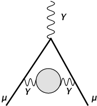
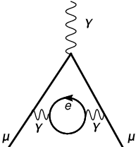
In QED diagrams with internal fermion loops arise starting from two-loop order, where the fermion type of the internal loop can be in general different from the external muon. In the case that the internal fermion loop consists of an electron, logarithmic contributions of the type $\ln(M_{\mu}/M_{e})$ arise, where $M_{\mu}$ is the mass of the muon and $M_{e}$ the mass of the electron. In view of the large mass ratio $M_{\mu}/M_{e}\sim 200$ one expects these logarithms to play a dominant role. These logarithmically enhanced contributions arise on the one hand from the insertion of the electron vacuum polarization (eVP) into the first order muon vertex diagram, shown in Fig. 1(a), but they can on the other hand also appear through light-by-light (LBL) scattering diagrams. Examples for both diagram types are shown in Fig. 2.

At five-loop level all diagrams contributing to $a^{theo}_{\mu}$ can be decomposed into six supersets, which can be further subdivided into 32 gauge invariant subsets[13]. These supersets have been computed numerically in Ref. [4]. For a few subsets also analytical results were obtained in Refs. [14, 15].

In this work we compute analytically the asymptotic limit of the photon propagator with massive electron loops and photon exchanges at four-loop order in two renormalization schemes: the $\overline{\mbox{MS}}$-one and the classical on-shell scheme. The calculation is then employed for the derivation of the $\overline{\mbox{MS}}$–on-shell relation of the fine structure constant $\alpha$ at four-loop order. This relation allows the conversion of observables, conveniently computed in the $\overline{\mbox{MS}}$ scheme, into the on-shell(OS) scheme or vice versa. These conversion relations combined with the recently published QED $\beta$-function in the $\overline{\mbox{MS}}$ scheme at five loops [1] are then used to derive the complete five-loop contribution to the QED $\beta$-function in the OS scheme as well as the momentum-dependent part of the polarization function in both the $\overline{\mbox{MS}}$ and OS scheme at five loops. These new four-loop and five-loop results are subsequently used to determine analytically $a^{\scriptsize asymp}_{\mu}$ at five loops as well as some genuinely six-loop contributions to $a^{\scriptsize asymp}_{\mu}$. This will constitute a new analytical result for several gauge invariant subclasses of the five-loop QED muon anomaly and will serve as a check for some already known numerical results.

The outline of the paper is as follows: in Section 2 we introduce our notations and conventions. In Section 3 we discuss the methods of calculation and present the results for the vacuum polarization function for small and large $Q^{2}$ in $\overline{\mbox{MS}}$ and on-shell scheme. In the next Section we use these results to derive the conversion formulas between the QED charge, renormalized in $\overline{\mbox{MS}}$ and on-shell schemes. In Section 5 the polarization operator at five loops is discussed. In the following Section 6 we derive the complete five-loop contribution to the QED $\beta$-function in the OS scheme as well as the momentum-dependent part of the polarization function in both $\overline{\mbox{MS}}$ and OS schemes at five loops. In Sections 7 and 8 we analytically compute all asymptotic contributions to the muon anomaly at five loops and logarithmically enhanced ones at six loops respectively. Finally in Section 9 we close with a brief summary and our conclusions.

We consider QED with $N$ identical fermions with mass $m$. The $\overline{\mbox{MS}}$ renormalized photon propagator $\overline{D}^{\mu\nu}_{R}$ is related to the photon polarization function $\overline{\Pi}(-q^{2}/\mu^{2},\overline{m}/\mu,\overline{\alpha})$ in the standard way:

$$\overline{D}^{\mu\nu}_{R}(-q^{2},\overline{m},\overline{\alpha},\mu)=\frac{-g_{\mu\nu}}{-q^{2}}\frac{1}{1+\overline{\Pi}(\frac{-q^{2}}{\mu^{2}},\frac{\overline{m}}{\mu},\overline{\alpha})}+q^{\mu}q^{\nu}\ \ \mbox{terms}{},$$

(1)

where $\overline{\alpha}\equiv\alpha^{{\scriptsize\overline{\rm MS}}}(\mu)$, $\overline{m}\equiv\overline{m}^{{\scriptsize\overline{\rm MS}}}(\mu)$ and $\mu$ are the running coupling constant, the fermion mass and normalization scale in $\overline{\mbox{MS}}$ scheme respectively. The symbol $q$ denotes the external Minkowskian momentum of the polarization function. At four-loop order the appearing self-energy diagrams can be classified into four classes: singlet and non-singlet type diagrams, where the non-singlet ones can be again decomposed with respect to the number of inserted closed fermion loops. Some example diagrams are shown in Fig. 3.

As is well-known the $\overline{\mbox{MS}}$ renormalized photon self-energy does not have any power-not suppressed terms of the type $\ln(\overline{m}^{2})$ in the limit of large $Q^{2}\equiv-q^{2}$. They appear only at order $\mathcal{O}(\overline{m}^{4}/Q^{4})$ of the large Q asymptotic expansion (see, e.g. Ref. [16]). This allows to define the asymptotic part of the polarization function $\overline{\Pi}$ in the limit $\overline{m}\to 0$ as follows:

$$\overline{\Pi}^{\mbox{\scriptsize asymp}}\bigg(\frac{-q^{2}}{\mu^{2}},\overline{\alpha}\bigg)\equiv\overline{\Pi}\bigg(\frac{Q^{2}}{\mu^{2}},\frac{\overline{m}}{\mu}=0,\overline{\alpha}\bigg){}.$$

(2)

The running of the coupling constant $\overline{\alpha}(\mu)$ is governed by the corresponding evolution equation of the form:

$$\mu^{2}\frac{d}{d\mu^{2}}\ln\overline{\alpha}=\overline{\beta}(\overline{\alpha}){}.$$

(3)

The evolution equation for the polarization function can be directly obtained from the fundamental concept of the scheme-invariant charge [17, 18], defined through

$${\overline{\alpha}\over 1+\overline{\Pi}(\frac{-q^{2}}{\mu^{2}},\frac{\overline{m}}{\mu},\overline{\alpha})}{}.$$

(4)

For the case of the asymptotic polarization function the evolution equation assumes the following, particularly simple form:

$$\Biggl\{\mu^{2}\frac{\partial}{\partial\mu^{2}}+\overline{\beta}(\overline{\alpha})\,\left(\overline{\alpha}\,\frac{\partial}{\partial\overline{\alpha}}-1\right)\Biggr\}\,(1+\overline{\Pi}^{\mbox{\scriptsize asymp}}(Q^{2}/\mu^{2},\overline{\alpha}))=0{}.$$

(5)

Recently the QED $\beta$-function, as defined in the $\overline{\mbox{MS}}$-scheme, has been evaluated to five-loop order [1]. For convenience of the reader we provide the corresponding result below²² 2 Note, please, that the function $\overline{\beta}(\overline{\alpha})$ is related to $\beta^{QED}(A)$ as given in Eq. (4.7) of [1] as follows: $\overline{\beta}(\overline{\alpha})\equiv\left(\beta^{QED}(A)/A\right)|_{A=\overline{\alpha}/(4\pi)}$. :

			$\displaystyle\overline{\beta}(\overline{\alpha})=\frac{4\,N}{3}\frac{\overline{\alpha}}{4\,\pi}{+}4\,N\left(\frac{\overline{\alpha}}{4\,\pi}\right)^{2}-\left(\frac{\overline{\alpha}}{4\,\pi}\right)^{3}\left[2\,N+\frac{44}{9}\,N^{2}\right]$		(6)
		$\displaystyle{+}$	$\displaystyle\left(\frac{\overline{\alpha}}{4\,\pi}\right)^{4}\left[-46\,N+\frac{760}{27}\,N^{2}-\frac{832}{9}\,\zeta_{3}\,N^{2}-\frac{1232}{243}\,N^{3}\right]$
		$\displaystyle{+}$	$\displaystyle\left(\frac{\overline{\alpha}}{4\,\pi}\right)^{5}\Biggl(\,N\left[\frac{4157}{6}+128\zeta_{3}\right]{+}\,N^{2}\left[-\frac{7462}{9}-992\zeta_{3}+2720\zeta_{5}\right]$
		$\displaystyle{+}$	$\displaystyle\,N^{3}\left[-\frac{21758}{81}+\frac{16000}{27}\zeta_{3}-\frac{416}{3}\zeta_{4}-\frac{1280}{3}\zeta_{5}\right]{+}\,N^{4}\left[\frac{856}{243}+\frac{128}{27}\zeta_{3}\right]\Biggr){}.$

Traditionally in calculations of leptonic($\ell$) anomalies $a_{\ell}$ the classical OS scheme is employed. In this subtraction scheme the QED is parametrized with two variables, namely, the fine structure constant $\alpha\equiv\alpha^{OS}$, equal to the invariant charge (4) at zero momentum transfer, and the pole mass $M$ of the fermion. The corresponding normalization condition for the OS polarization function $\Pi(-q^{2}/M^{2},\alpha)\equiv\Pi^{OS}(-q^{2}/M^{2},\alpha)$ is:

$$\Pi(-q^{2}=0,M,\alpha)\equiv 0{}.$$

(7)

The asymptotic polarization function $\Pi^{asymp}(Q^{2}/M^{2},\alpha)$ is obtained from $\Pi(Q^{2}/M^{2},\alpha)$ by discarding in every order of perturbation theory all power suppressed terms in the limit of $M\to 0$. Finally, according to Ref. [8] one obtains the asymptotic part of the muon anomaly (related to the vacuum polarization diagrams) through the relation:

$$a^{\mbox{\scriptsize asymp}}_{\mu}={\alpha\over\pi}\int_{0}^{1}\!dx\,(1-x)\,\left[d^{\mbox{\scriptsize asymp}}_{R}\left({x^{2}\over 1-x}{M_{\mu}^{2}\over M_{e}^{2}},\alpha\right)-1\right],$$

(8)

where

$$d^{\mbox{\scriptsize asymp}}_{R}(Q^{2}/M^{2},\alpha)={1\over 1+\Pi^{\mbox{\scriptsize asymp}}(Q^{2}/M^{2},\alpha)}.$$

(9)

The asymptotic limit $\overline{m}\to 0$ requires the computation of massless propagators, whereas the limit $q^{2}\to 0$ leads to the evaluation of massive tadpole diagrams. The perturbative expansion of the vacuum polarization function in the fine structure constant in the two cases is conveniently defined by:

$$\overline{\Pi}(Q^{2},\overline{m}^{2}=0,\overline{\alpha})=\sum_{i}\overline{\Pi}^{(i)}(\ell_{\mu Q})\left(\frac{\overline{\alpha}(\mu)}{\pi}\right)^{i}$$

(10)

and

$$\overline{\Pi}(Q^{2}=0,\overline{m}^{2},\overline{\alpha})=\sum_{i}\overline{\Pi}^{(i)}(q=0,\ell_{{\mu}m})\left(\frac{\overline{\alpha}(\mu)}{\pi}\right)^{i}{},$$

(11)

where $\ell_{{\mu}Q}=\ln(\mu^{2}/Q^{2})$ and $\ell_{{\mu}m}=\ln(\mu^{2}/\overline{m}^{2})$. In both cases the computation has been performed with FORM [19, 20, 21] based programs. The four-loop QED diagrams contributing to the electron polarization function have been generated with the program QGRAF[22].

The four-loop massless propagators can be reduced to 28 master integrals. The reduction of four-loop massless propagators has been done by evaluating sufficiently many terms of the $1/D$ expansion [23] of the corresponding coefficient functions [24]. The master integrals are known analytically from [25, 26].

In the low $Q^{2}$ limit all appearing tadpole diagrams have been reduced to master integrals with the help of Laporta’s algorithm [27, 28]. The arising polynomials in the space-time dimension $d=4-2\,\varepsilon$ have been simplified with the program FERMAT [29]. The remaining master integrals are known analytically to sufficient high order in $\varepsilon$ and have been taken from Refs. [30, 31, 32, 33, 34, 35, 36, 37, 38].

For the large $Q^{2}$ limit our result, renormalized completely in the $\overline{\mbox{MS}}$ scheme, reads:

	$\displaystyle\overline{\Pi}^{(1)}(\ell_{\mu Q})$	$\displaystyle=$	$\displaystyle N\left[\frac{5}{9}+\frac{1}{3}\ell_{\mu Q}\right]{},$		(12)
	$\displaystyle\overline{\Pi}^{(2)}(\ell_{\mu Q})$	$\displaystyle=$	$\displaystyle\,N\left[\frac{55}{48}-\zeta_{3}+\frac{1}{4}\ell_{\mu Q}\right]{},$		(13)
	$\displaystyle\overline{\Pi}^{(3)}(\ell_{\mu Q})$	$\displaystyle=$	$\displaystyle N\left[-\frac{143}{288}-\frac{37}{24}\zeta_{3}+\frac{5}{2}\zeta_{5}-\frac{1}{32}\ell_{\mu Q}\right]$		(14)
		$\displaystyle{+}$	$\displaystyle\,N^{2}\left[-\frac{3701}{2592}+\frac{19}{18}\zeta_{3}-\frac{11}{24}\ell_{\mu Q}+\frac{1}{3}\zeta_{3}\ell_{\mu Q}-\frac{1}{24}\ell_{\mu Q}^{2}\right]{},$
	$\displaystyle\overline{\Pi}^{(4)}(\ell_{\mu Q})$	$\displaystyle=$	$\displaystyle\,N\left[-\frac{31}{768}+\frac{13}{32}\zeta_{3}+\frac{245}{32}\zeta_{5}-\frac{35}{4}\,\zeta_{7}-\frac{23}{128}\ell_{\mu Q}\right]$		(15)
		$\displaystyle{+}$	$\displaystyle\,N^{2}\left[-\frac{7505}{41472}+\frac{11}{8640}\,\pi^{4}+\frac{1553}{216}\zeta_{3}-\,\zeta_{3}^{2}-\frac{125}{18}\zeta_{5}-\frac{29}{192}\ell_{\mu Q}\right.$
			$\displaystyle\left.\phantom{+\,N^{2}}+\frac{19}{12}\zeta_{3}\ell_{\mu Q}-\frac{5}{3}\zeta_{5}\ell_{\mu Q}-\frac{1}{48}\ell_{\mu Q}^{2}\right]$
		$\displaystyle{+}$	$\displaystyle\,N^{2}\,{\bf si}\,\left[\frac{431}{432}-\frac{1}{360}\,\pi^{4}-\frac{21}{16}\zeta_{3}-\frac{2}{3}\,\zeta_{3}^{2}+\frac{5}{4}\zeta_{5}+\frac{11}{36}\ell_{\mu Q}-\frac{2}{3}\zeta_{3}\ell_{\mu Q}\right]$
		$\displaystyle{+}$	$\displaystyle\,N^{3}\left[\frac{196513}{93312}-\frac{809}{648}\zeta_{3}-\frac{5}{9}\zeta_{5}+\frac{151}{162}\ell_{\mu Q}-\frac{19}{27}\zeta_{3}\ell_{\mu Q}+\frac{11}{72}\ell_{\mu Q}^{2}\right.$
			$\displaystyle\left.\phantom{+\,N^{3}}-\frac{1}{9}\zeta_{3}\ell_{\mu Q}^{2}+\frac{1}{108}\ell_{\mu Q}^{3}\right]{},$

with $\zeta_{n}$ being the Riemann zeta-function defined by:

$$\zeta_{n}=\sum_{k=1}^{\infty}{1\over k^{n}}$$

(16)

and $\ell_{\mu Q}=\ln(\frac{\mu^{2}}{Q^{2}})$. The symbol ${\bf{si}}$ is here and in the following equal one and serves only as a separator in order to display the singlet contributions, originating from diagrams of the type as shown in Fig. 3(s), separately. As stated above, no logarithms of the type $\ln(\overline{m}^{2})$ appear in this result. However, in the low $Q^{2}=0$ case the renormalized vacuum polarization function does contain logarithms of the type $\ell_{\mu m}=\ln({\mu^{2}\over\overline{m}^{2}})$. In this limit our analytical result, renormalized in the $\overline{\mbox{MS}}$ scheme, reads:

	$\displaystyle\overline{\Pi}^{(1)}(q=0,\ell_{\mu m})$	$\displaystyle=$	$\displaystyle N\left[\frac{1}{3}\,\ell_{\mu m}\,\right]{},$		(17)
	$\displaystyle\overline{\Pi}^{(2)}(q=0,\ell_{\mu m})$	$\displaystyle=$	$\displaystyle N\left[\frac{13}{48}-\frac{1}{4}\,\ell_{\mu m}\,\right]{},$		(18)
	$\displaystyle\overline{\Pi}^{(3)}(q=0,\ell_{\mu m})$	$\displaystyle=$	$\displaystyle N\left[\frac{97}{288}-\frac{95}{192}\zeta_{3}+\frac{9}{32}\,\ell_{\mu m}\,\right]$		(19)
		$\displaystyle{+}$	$\displaystyle\,N^{2}\left[-\frac{103}{1296}+\frac{7}{64}\zeta_{3}-\frac{1}{36}\,\ell_{\mu m}\,+\frac{1}{24}\,\ell_{\mu m}^{2}\right]{},$

	$\displaystyle\overline{\Pi}^{(4)}(q=0,\ell_{\mu m})=$				(20)
			$\displaystyle N\left[-\frac{37441}{34560}+\frac{58001}{129600}\,\pi^{4}-\frac{7549}{320}\zeta_{3}+\frac{3429}{160}\zeta_{5}-\frac{157}{128}\,\ell_{\mu m}\,-\frac{106}{675}\,\pi^{4}\ln\!{(2)}\,\right.$
			$\displaystyle\left.+\frac{1919}{1080}\,\pi^{2}\ln^{\!2}\!{(2)}\,-\frac{32}{135}\,\pi^{2}\ln^{\!3}\!{(2)}\,-\frac{1919}{1080}\ln^{\!4}\!{(2)}\,+\frac{32}{225}\ln^{\!5}\!{(2)}\,-\frac{1919}{45}\,a_{4}-\frac{256}{15}\,a_{5}\right]$
		$\displaystyle{+}$	$\displaystyle\,N^{2}\left[-\frac{2261597}{1036800}+\frac{29737}{129600}\,\pi^{4}-\frac{123149}{10800}\zeta_{3}-\frac{41}{576}\,\ell_{\mu m}\,+\frac{13}{96}\zeta_{3}\,\ell_{\mu m}\,-\frac{1}{8}\,\ell_{\mu m}^{2}\right.$
			$\displaystyle\left.\phantom{+\,N^{2}}+\frac{437}{540}\,\pi^{2}\ln^{\!2}\!{(2)}\,-\frac{437}{540}\ln^{\!4}\!{(2)}\,-\frac{874}{45}\,a_{4}\right]$
		$\displaystyle{+}$	$\displaystyle\,N^{2}\,{\bf si}\,\left[\frac{2411}{5040}+\frac{2189}{17280}\,\pi^{4}-\frac{6779}{1120}\zeta_{3}-\frac{5}{12}\zeta_{5}+\frac{11}{36}\,\ell_{\mu m}\,-\frac{2}{3}\zeta_{3}\,\ell_{\mu m}\,\right.$
			$\displaystyle\left.\phantom{+\,N^{2}\,{\bf si}\,}+\frac{73}{144}\,\pi^{2}\ln^{\!2}\!{(2)}\,-\frac{73}{144}\ln^{\!4}\!{(2)}\,-\frac{73}{6}\,a_{4}\right]$
		$\displaystyle{+}$	$\displaystyle\,N^{3}\left[\frac{610843}{3265920}-\frac{661}{3780}\zeta_{3}+\frac{113}{1296}\,\ell_{\mu m}\,-\frac{7}{96}\zeta_{3}\,\ell_{\mu m}\,+\frac{1}{108}\,\ell_{\mu m}^{2}-\frac{1}{108}\,\ell_{\mu m}^{3}\right]{},$

where the polylogarithm function $\mbox{Li}_{n}(1/2)$ is defined by:

$$a_{n}=\mbox{Li}_{n}(1/2)=\sum_{k=1}^{\infty}{1\over 2^{k}k^{n}}\,.$$

(21)

In the next step we convert the results of Eqs. (12)-(15) from the $\overline{\mbox{MS}}$ into the on-shell scheme in order to obtain the asymptotic limit of the polarization function $\Pi^{\mbox{\scriptsize asymp}}(Q^{2},M^{2},\alpha)$ in OS scheme. The scheme independence of the invariant charge directly leads to the relation:

$$\Pi^{\mbox{\scriptsize asymp}}(Q^{2}/M^{2},\alpha)=\frac{\alpha}{\overline{\alpha}}\Biggl(1+\overline{\Pi}^{\mbox{\scriptsize asymp}}(Q^{2}/\mu^{2},\overline{\alpha})\Biggr)-1{},$$

(22)

where it is understood that the running $\overline{\alpha}$ on the r.h.s. is converted into the on-shell coupling constant $\alpha$. The corresponding conversion relation is given in the next Section 4.

In analogy to Eqs. (10) and (11) the expansion in the on-shell fine structure constant $\alpha$ of $\Pi^{\mbox{\scriptsize asymp}}(Q^{2},M^{2},\alpha)$ is defined by:

$$\Pi^{\mbox{\scriptsize asymp}}(Q^{2}/M^{2},\alpha)=\sum_{i}{\Pi}^{\mbox{\scriptsize asymp},(i)}(\ell_{MQ})\left(\frac{\alpha}{\pi}\right)^{i}{}.$$

(23)

The asymptotic limit of the polarization function in the OS scheme is given by ($\ell_{MQ}=\ln(\frac{M^{2}}{Q^{2}})$):

	$\displaystyle\Pi^{\mbox{\scriptsize asymp},(1)}(\ell_{MQ})$	$\displaystyle=$	$\displaystyle N\left[\frac{5}{9}+\frac{1}{3}\ell_{MQ}\right]{},$		(24)
	$\displaystyle\Pi^{\mbox{\scriptsize asymp},(2)}(\ell_{MQ})$	$\displaystyle=$	$\displaystyle N\left[\frac{5}{24}-\zeta_{3}+\frac{1}{4}\ell_{MQ}\right]{},$		(25)
	$\displaystyle\Pi^{\mbox{\scriptsize asymp},(3)}(\ell_{MQ})$	$\displaystyle=$	$\displaystyle\,N\left[-\frac{121}{192}-\frac{5}{24}\,\pi^{2}-\frac{99}{64}\zeta_{3}+\frac{5}{2}\zeta_{5}-\frac{1}{32}\ell_{MQ}+\frac{1}{3}\,\pi^{2}\ln\!{(2)}\,\right]$		(26)
		$\displaystyle{+}$	$\displaystyle\,N^{2}\left[-\frac{307}{864}-\frac{1}{9}\,\pi^{2}+\frac{545}{576}\zeta_{3}-\frac{11}{24}\ell_{MQ}+\frac{1}{3}\zeta_{3}\ell_{MQ}-\frac{1}{24}\ell_{MQ}^{2}\right]{},$

			$\displaystyle\Pi^{\mbox{\scriptsize asymp},(4)}(\ell_{MQ})=N\left[-\frac{71189}{34560}-\frac{157}{72}\,\pi^{2}-\frac{59801}{129600}\,\pi^{4}+\frac{6559}{320}\zeta_{3}-\frac{1}{24}\,\pi^{2}\zeta_{3}-\frac{1603}{120}\zeta_{5}\right.$		(27)
			$\displaystyle\left.\phantom{+\,N}-\frac{35}{4}\,\zeta_{7}-\frac{23}{128}\ell_{MQ}+\frac{59}{12}\,\pi^{2}\ln\!{(2)}\,+\frac{106}{675}\,\pi^{4}\ln\!{(2)}\,-\frac{1559}{1080}\,\pi^{2}\ln^{\!2}\!{(2)}\,+\frac{32}{135}\,\pi^{2}\ln^{\!3}\!{(2)}\,\right.$
			$\displaystyle\left.\phantom{+\,N}+\frac{1559}{1080}\ln^{\!4}\!{(2)}\,-\frac{32}{225}\ln^{\!5}\!{(2)}\,+\frac{1559}{45}\,a_{4}+\frac{256}{15}\,a_{5}\right]$
		$\displaystyle{+}$	$\displaystyle\,N^{2}\left[\frac{3361}{900}-\frac{179}{324}\,\pi^{2}-\frac{2161}{10800}\,\pi^{4}+\frac{29129}{1800}\zeta_{3}-\,\zeta_{3}^{2}-\frac{125}{18}\zeta_{5}\right.$
			$\displaystyle\left.\phantom{+\,N^{2}}+\frac{1}{12}\ell_{MQ}+\frac{19}{12}\zeta_{3}\ell_{MQ}-\frac{5}{3}\zeta_{5}\ell_{MQ}-\frac{1}{48}\ell_{MQ}^{2}+\frac{16}{27}\,\pi^{2}\ln\!{(2)}\,-\frac{53}{60}\,\pi^{2}\ln^{\!2}\!{(2)}\,\right.$
			$\displaystyle\left.\phantom{+\,N^{2}}+\frac{53}{60}\ln^{\!4}\!{(2)}\,+\frac{106}{5}\,a_{4}\right]$
		$\displaystyle{+}$	$\displaystyle\,N^{2}\,{\bf si}\,\left[\frac{1963}{3780}-\frac{2237}{17280}\,\pi^{4}+\frac{5309}{1120}\zeta_{3}-\frac{2}{3}\,\zeta_{3}^{2}+\frac{5}{3}\zeta_{5}+\frac{11}{36}\ell_{MQ}\right.$
			$\displaystyle\left.\phantom{+\,N^{2}\,{\bf si}\,}-\frac{2}{3}\zeta_{3}\ell_{MQ}-\frac{73}{144}\,\pi^{2}\ln^{\!2}\!{(2)}\,+\frac{73}{144}\ln^{\!4}\!{(2)}\,+\frac{73}{6}\,a_{4}\right]$
		$\displaystyle{+}$	$\displaystyle\,N^{3}\left[\frac{75259}{68040}+\frac{8}{405}\,\pi^{2}-\frac{15109}{22680}\zeta_{3}-\frac{5}{9}\zeta_{5}+\frac{151}{162}\ell_{MQ}-\frac{19}{27}\zeta_{3}\ell_{MQ}\right.$
			$\displaystyle\left.\phantom{+\,N^{3}}+\frac{11}{72}\ell_{MQ}^{2}-\frac{1}{9}\zeta_{3}\ell_{MQ}^{2}+\frac{1}{108}\ell_{MQ}^{3}\right]{}.$

The results displayed in Eqs. (24)-(26) (as well as those in Eqs. (12)-(14), (17)-(19)) are known since long (see, e.g. [9] and references therein). Note that all terms proportional to $\ell_{MQ}$ in Eq. (27) follow in an easy way from renormalization group arguments as explained in [8]. In addition, in the process of constructing $d_{R}^{\mbox{\scriptsize asymp}}$ one should invert the power series for $(1+\Pi^{\mbox{\scriptsize asymp}})$, which also produces childishly-easy-to-compute factorizable fourth order contributions to $d_{R}^{\mbox{\scriptsize asymp}}$ like $\alpha^{4}\,\Pi^{\mbox{\scriptsize asymp},(2)}\,\Pi^{\mbox{\scriptsize asymp},(2)}$ and so on (see e.g. [39] and references therein). However, to include power suppressed terms of order $(M/Q)^{n}$ to $\Pi^{\mathrm{OS}}$ is much less trivial even for the factorizable contributions [40, 41]. In fact, the second work also provides power suppressed contributions to the muon anomaly from factorizable diagrams of type I(a) (see Fig. 4) for the cases when leptons circulated in closed loops could be not just electrons but also muons and tau-leptons in different combinations.

Let us define the conversion factor $C_{\alpha\overline{\alpha}}$, which converts the fine structure constant $\overline{\alpha}$ in $\overline{\mbox{MS}}$ scheme into $\alpha$ in OS scheme: $\alpha=C_{\alpha\overline{\alpha}}\,\overline{\alpha}$. The conversion factor $C_{\alpha\overline{\alpha}}$ has a perturbative expansion in $\overline{\alpha}$ defined by:

$$C_{\alpha\overline{\alpha}}=1+\sum_{i\geq 1}C_{\alpha\overline{\alpha}}^{(i)}\left(\frac{\overline{\alpha}(\mu)}{\pi}\right)^{i}.$$

(28)

The expansion coefficients $C_{\alpha\overline{\alpha}}^{(i)}$ can be obtained by evaluating Eq. (22) at $Q^{2}=0$ and using Eq. (7). On the r.h.s. of this equation we insert the results of Eqs. (11), (17)-(20) and expand in $\overline{\alpha}$ up to four-loop order. In addition, one should use the relation to convert the $\overline{\mbox{MS}}$-mass $\overline{m}(\mu)$ to the on-shell mass $M$, which is known from Refs. [42, 43] to three-loop order. For the case of QED it is given in Appendix A.

The different orders $C_{\alpha\overline{\alpha}}^{(i)}$ read:

	$\displaystyle C_{\alpha\overline{\alpha}}^{(1)}(\ell_{\mu M})=$				(29)
		$\displaystyle{+}$	$\displaystyle\,N\left[-\frac{1}{3}\,\ell_{\mu M}\,\right]{},$

	$\displaystyle C_{\alpha\overline{\alpha}}^{(2)}(\ell_{\mu M})=$				(30)
		$\displaystyle{+}$	$\displaystyle\,N\left[-\frac{15}{16}-\frac{1}{4}\,\ell_{\mu M}\,\right]$
		$\displaystyle{+}$	$\displaystyle\,N^{2}\left[\frac{1}{9}\,\ell_{\mu M}^{2}\right]{},$

	$\displaystyle C_{\alpha\overline{\alpha}}^{(3)}(\ell_{\mu M})=$				(31)
		$\displaystyle{+}$	$\displaystyle\,N\left[-\frac{77}{576}-\frac{5}{24}\,\pi^{2}-\frac{1}{192}\zeta_{3}+\frac{1}{32}\,\ell_{\mu M}\,+\frac{1}{3}\,\pi^{2}\ln\!{(2)}\,\right]$
		$\displaystyle{+}$	$\displaystyle\,N^{2}\left[\frac{695}{648}-\frac{1}{9}\,\pi^{2}-\frac{7}{64}\zeta_{3}+\frac{73}{72}\,\ell_{\mu M}\,+\frac{5}{24}\,\ell_{\mu M}^{2}\right]$
		$\displaystyle{+}$	$\displaystyle\,N^{3}\left[-\frac{1}{27}\,\ell_{\mu M}^{3}\right]{},$

	$\displaystyle C_{\alpha\overline{\alpha}}^{(4)}(\ell_{\mu M})=$				(32)
		$\displaystyle{+}$	$\displaystyle\,N\left[-\frac{34897}{17280}-\frac{157}{72}\,\pi^{2}-\frac{59801}{129600}\,\pi^{4}+\frac{6429}{320}\zeta_{3}-\frac{1}{24}\,\pi^{2}\zeta_{3}-\frac{10087}{480}\zeta_{5}\right.$
			$\displaystyle\left.\phantom{+\,N}+\frac{23}{128}\,\ell_{\mu M}\,+\frac{59}{12}\,\pi^{2}\ln\!{(2)}\,+\frac{106}{675}\,\pi^{4}\ln\!{(2)}\,-\frac{1559}{1080}\,\pi^{2}\ln^{\!2}\!{(2)}\,\right.$
			$\displaystyle\left.\phantom{+\,N}+\frac{32}{135}\,\pi^{2}\ln^{\!3}\!{(2)}\,+\frac{1559}{1080}\ln^{\!4}\!{(2)}\,-\frac{32}{225}\ln^{\!5}\!{(2)}\,+\frac{1559}{45}\,a_{4}+\frac{256}{15}\,a_{5}\right]$
		$\displaystyle{+}$	$\displaystyle\,N^{2}\left[\frac{4768247}{1036800}-\frac{179}{324}\,\pi^{2}-\frac{8699}{43200}\,\pi^{4}+\frac{107249}{10800}\zeta_{3}+\frac{1861}{1728}\,\ell_{\mu M}\,+\frac{5}{18}\,\pi^{2}\,\ell_{\mu M}\,\right.$
			$\displaystyle\left.\phantom{+\,N^{2}}-\frac{43}{144}\zeta_{3}\,\ell_{\mu M}\,+\frac{1}{16}\,\ell_{\mu M}^{2}+\frac{16}{27}\,\pi^{2}\ln\!{(2)}\,-\frac{4}{9}\,\pi^{2}\,\ell_{\mu M}\,\ln\!{(2)}\,-\frac{53}{60}\,\pi^{2}\ln^{\!2}\!{(2)}\,\right.$
			$\displaystyle\left.\phantom{+\,N^{2}}+\frac{53}{60}\ln^{\!4}\!{(2)}\,+\frac{106}{5}\,a_{4}\right]$
		$\displaystyle{+}$	$\displaystyle\,N^{2}\,{\bf si}\,\left[-\frac{2411}{5040}-\frac{2189}{17280}\,\pi^{4}+\frac{6779}{1120}\zeta_{3}+\frac{5}{12}\zeta_{5}-\frac{11}{36}\,\ell_{\mu M}\,+\frac{2}{3}\zeta_{3}\,\ell_{\mu M}\,\right.$
			$\displaystyle\left.\phantom{+\,N^{2}\,{\bf si}\,}-\frac{73}{144}\,\pi^{2}\ln^{\!2}\!{(2)}\,+\frac{73}{144}\ln^{\!4}\!{(2)}\,+\frac{73}{6}\,a_{4}\right]$
		$\displaystyle{+}$	$\displaystyle\,N^{3}\left[-\frac{3265523}{3265920}+\frac{8}{405}\,\pi^{2}+\frac{2201}{3780}\zeta_{3}-\frac{5483}{3888}\,\ell_{\mu M}\,+\frac{4}{27}\,\pi^{2}\,\ell_{\mu M}\,+\frac{7}{48}\zeta_{3}\,\ell_{\mu M}\,\right.$
			$\displaystyle\left.\phantom{+\,N^{3}}-\frac{101}{144}\,\ell_{\mu M}^{2}-\frac{13}{108}\,\ell_{\mu M}^{3}\right]$
		$\displaystyle{+}$	$\displaystyle\,N^{4}\left[\frac{1}{81}\,\ell_{\mu M}^{4}\right]{},$

with $\ell_{{\mu}M}=\ln(\mu^{2}/M^{2})$. On the other hand the inverse conversion factor $C_{\overline{\alpha}{\alpha}}$, which allows a conversion from the $\overline{\mbox{MS}}$ to the on-shell scheme $\overline{\alpha}=C_{\overline{\alpha}{\alpha}}\,\alpha$ is useful as well. In analogy to Eq. (28) the perturbative expansion in $\alpha$ of $C_{\overline{\alpha}{\alpha}}$ is defined as:

$$C_{\overline{\alpha}\alpha}=1+\sum_{i\geq 1}C_{\overline{\alpha}\alpha}^{(i)}\left(\frac{{\alpha}}{\pi}\right)^{i}.$$

(33)

Proceeding like in the previous case and inverting the series obtained with the help of Eq. (22), we find:

	$\displaystyle C_{\overline{\alpha}\alpha}^{(1)}(\ell_{\mu M})=$				(34)
		$\displaystyle{+}$	$\displaystyle\,N\left[\frac{1}{3}\,\ell_{\mu M}\,\right]{},$

	$\displaystyle C_{\overline{\alpha}\alpha}^{(2)}(\ell_{\mu M})=$				(35)
		$\displaystyle{+}$	$\displaystyle\,N\left[\frac{15}{16}+\frac{1}{4}\,\ell_{\mu M}\,\right]$
		$\displaystyle{+}$	$\displaystyle\,N^{2}\left[\frac{1}{9}\,\ell_{\mu M}^{2}\right]{},$

	$\displaystyle C_{\overline{\alpha}\alpha}^{(3)}(\ell_{\mu M})=$				(36)
		$\displaystyle{+}$	$\displaystyle\,N\left[\frac{77}{576}+\frac{5}{24}\,\pi^{2}+\frac{1}{192}\zeta_{3}-\frac{1}{32}\,\ell_{\mu M}\,-\frac{1}{3}\,\pi^{2}\ln\!{(2)}\,\right]$
		$\displaystyle{+}$	$\displaystyle\,N^{2}\left[-\frac{695}{648}+\frac{1}{9}\,\pi^{2}+\frac{7}{64}\zeta_{3}+\frac{79}{144}\,\ell_{\mu M}\,+\frac{5}{24}\,\ell_{\mu M}^{2}\right]$
		$\displaystyle{+}$	$\displaystyle\,N^{3}\left[\frac{1}{27}\,\ell_{\mu M}^{3}\right]{},$

	$\displaystyle C_{\overline{\alpha}\alpha}^{(4)}(\ell_{\mu M})=$				(37)
		$\displaystyle{+}$	$\displaystyle\,N\left[\frac{34897}{17280}+\frac{157}{72}\,\pi^{2}+\frac{59801}{129600}\,\pi^{4}-\frac{6429}{320}\zeta_{3}+\frac{1}{24}\,\pi^{2}\zeta_{3}+\frac{10087}{480}\zeta_{5}\right.$
			$\displaystyle\left.\phantom{+\,N}-\frac{23}{128}\,\ell_{\mu M}\,-\frac{59}{12}\,\pi^{2}\ln\!{(2)}\,-\frac{106}{675}\,\pi^{4}\ln\!{(2)}\,+\frac{1559}{1080}\,\pi^{2}\ln^{\!2}\!{(2)}\,\right.$
			$\displaystyle\left.\phantom{+\,N}-\frac{32}{135}\,\pi^{2}\ln^{\!3}\!{(2)}\,-\frac{1559}{1080}\ln^{\!4}\!{(2)}\,+\frac{32}{225}\ln^{\!5}\!{(2)}\,-\frac{1559}{45}\,a_{4}-\frac{256}{15}\,a_{5}\right]$
		$\displaystyle{+}$	$\displaystyle\,N^{2}\left[-\frac{2034497}{1036800}+\frac{179}{324}\,\pi^{2}+\frac{8699}{43200}\,\pi^{4}-\frac{107249}{10800}\zeta_{3}+\frac{1031}{1728}\,\ell_{\mu M}\,+\frac{5}{36}\,\pi^{2}\,\ell_{\mu M}\,\right.$
			$\displaystyle\left.\phantom{+\,N^{2}}+\frac{89}{288}\zeta_{3}\,\ell_{\mu M}\,+\frac{1}{16}\,\ell_{\mu M}^{2}-\frac{16}{27}\,\pi^{2}\ln\!{(2)}\,-\frac{2}{9}\,\pi^{2}\,\ell_{\mu M}\,\ln\!{(2)}\,+\frac{53}{60}\,\pi^{2}\ln^{\!2}\!{(2)}\,\right.$
			$\displaystyle\left.\phantom{+\,N^{2}}-\frac{53}{60}\ln^{\!4}\!{(2)}\,-\frac{106}{5}\,a_{4}\right]$
		$\displaystyle{+}$	$\displaystyle\,N^{2}\,{\bf si}\,\left[\frac{2411}{5040}+\frac{2189}{17280}\,\pi^{4}-\frac{6779}{1120}\zeta_{3}-\frac{5}{12}\zeta_{5}+\frac{11}{36}\,\ell_{\mu M}\,-\frac{2}{3}\zeta_{3}\,\ell_{\mu M}\,\right.$
			$\displaystyle\left.\phantom{+\,N^{2}\,{\bf si}\,}+\frac{73}{144}\,\pi^{2}\ln^{\!2}\!{(2)}\,-\frac{73}{144}\ln^{\!4}\!{(2)}\,-\frac{73}{6}\,a_{4}\right]$
		$\displaystyle{+}$	$\displaystyle\,N^{3}\left[\frac{3265523}{3265920}-\frac{8}{405}\,\pi^{2}-\frac{2201}{3780}\zeta_{3}-\frac{2857}{3888}\,\ell_{\mu M}\,+\frac{2}{27}\,\pi^{2}\,\ell_{\mu M}\,+\frac{7}{96}\zeta_{3}\,\ell_{\mu M}\,\right.$
			$\displaystyle\left.\phantom{+\,N^{3}}+\frac{17}{72}\,\ell_{\mu M}^{2}+\frac{13}{108}\,\ell_{\mu M}^{3}\right]$
		$\displaystyle{+}$	$\displaystyle\,N^{4}\left[\frac{1}{81}\,\ell_{\mu M}^{4}\right]{}.$

In this section we will use the recent calculation [1] of $\overline{\beta}(\overline{\alpha})$ — the QED $\beta$-function in the $\overline{\mbox{MS}}$ scheme — at five-loop order to find the $Q$-dependent part of the five-loop contribution to the asymptotic polarization function in both $\overline{\mbox{MS}}$ and OS schemes.

References

• [1] P. Baikov, K. Chetyrkin, J. Kühn, and J. Rittinger, Vector Correlator in Massless QCD at Order O⁡(αs4)O(\alpha_{s}^{4}) and the QED beta-function at five loop, JHEP 1207 (2012) 017, [arXiv:1206.1284].
• [2] Muon G-2 Collaboration, G. W. Bennett et al., Final report of the muon E821 anomalous magnetic moment measurement at BNL, Phys. Rev. D73 (2006) 072003, [hep-ex/0602035].
• [3] Particle Data Group Collaboration, K. Nakamura et al., Review of particle physics, J. Phys. G37 (2010) 075021.
• [4] T. Aoyama, M. Hayakawa, T. Kinoshita, and M. Nio, Complete Tenth-Order QED Contribution to the Muon g-2, Phys. Rev. Lett. 109 (2012) 111808, [arXiv:1205.5370].
• [5] K. Melnikov and A. Vainshtein, Theory of the muon anomalous magnetic moment, Springer Tracts Mod. Phys. 216 (2006) 1–178.
• [6] F. Jegerlehner, The Anomalous Magnetic Moment of the Muon, Springer Tracts Mod. Phys. 226 (2008) 1–426.
• [7] F. Jegerlehner and A. Nyffeler, The Muon g-2, Phys. Rept. 477 (2009) 1–110, [arXiv:0902.3360].
• [8] B. Lautrup and E. de Rafael, The anomalous magnetic moment of the muon and short- distance behaviour of quantum electrodynamics, Nucl. Phys. B70 (1974) 317–350.
• [9] D. J. Broadhurst, A. L. Kataev, and O. V. Tarasov, Analytical on-shell QED results: Three loop vacuum polarization, four loop Beta function and the muon anomaly, Phys. Lett. B298 (1993) 445–452, [hep-ph/9210255].
• [10] T. Kinoshita, H. Kawai, and Y. Okamoto, Asymptotic photon propagator in massive QED and the muon anomalous magnetic moment, Phys. Lett. B254 (1991) 235–240.
• [11] P. A. Baikov and D. J. Broadhurst, Three-loop QED vacuum polarization and the four-loop muon anomalous magnetic moment, hep-ph/9504398.
• [12] R. Barbieri and E. Remiddi, Electron and Muon 1/2(g-2) from Vacuum Polarization Insertions, Nucl. Phys. B90 (1975) 233.
• [13] M. Nio, T. Aoyama, M. Hayakawa, and T. Kinoshita, QED contributions to muon g-2: Tenth-order graphs, Nucl. Phys. Proc. Suppl. 169 (2007) 238–243.
• [14] A. L. Kataev, Renormalization group and the five loop QED asymptotic contributions to the muon anomaly, Phys. Lett. B284 (1992) 401–409;
A. L. Kataev, Phys. Lett. B710 (2012) 710 (Erratum).
• [15] S. Laporta, Analytical and numerical contributions of some tenth order graphs containing vacuum polarization insertions to the muon (g-2) in QED, Phys. Lett. B328 (1994) 522–527, [hep-ph/9404204].
• [16] K. G. Chetyrkin, J. H. Kühn, and A. Kwiatkowski, QCD corrections to the e+​e−e^{+}e^{-} cross-section and the ZZ boson decay rate: Concepts and results, Phys. Rept. 277 (1996) 189–281.
• [17] N. N. Bogolyubov and D. V. Shirkov, Charge renormalization group in quantum field theory, Nuovo Cim. 3 (1956) 845–863.
• [18] D. Shirkov, The Bogolyubov renormalization group in theoretical and mathematical physics, hep-th/9903073.
• [19] J. A. M. Vermaseren, New features of FORM, math-ph/0010025.
• [20] J. A. M. Vermaseren, Tuning FORM with large calculations, Nucl. Phys. Proc. Suppl. 116 (2003) 343–347, [hep-ph/0211297].
• [21] M. Tentyukov and J. A. M. Vermaseren, Extension of the functionality of the symbolic program FORM by external software, Comput. Phys. Commun. 176 (2007) 385–405, [cs/0604052].
• [22] P. Nogueira, Automatic Feynman graph generation, J. Comput. Phys. 105 (1993) 279–289.
• [23] P. A. Baikov, A practical criterion of irreducibility of multi-loop Feynman integrals, Phys. Lett. B634 (2006) 325–329, [hep-ph/0507053].
• [24] P. A. Baikov, Explicit solutions of the 3–loop vacuum integral recurrence relations, Phys. Lett. B385 (1996) 404–410, [hep-ph/9603267].
• [25] P. A. Baikov and K. G. Chetyrkin, Four Loop Massless Propagators: an Algebraic Evaluation of All Master Integrals, Nucl. Phys. B837 (2010) 186–220, [arXiv:1004.1153].
• [26] R. N. Lee, A. V. Smirnov, and V. A. Smirnov, Master Integrals for Four-Loop Massless Propagators up to Transcendentality Weight Twelve, Nucl. Phys. B856 (2012) 95–110, [arXiv:1108.0732].
• [27] S. Laporta and E. Remiddi, The analytical value of the electron (g-2) at order α3\alpha^{3} in QED, Phys. Lett. B379 (1996) 283–291, [hep-ph/9602417].
• [28] S. Laporta, High-precision calculation of multi-loop Feynman integrals by difference equations, Int. J. Mod. Phys. A15 (2000) 5087–5159, [hep-ph/0102033].
• [29] R. H. Lewis, Fermat’s user guide, Fermat’s User Guide, http://www.bway.net/˜lewis/.
• [30] S. Laporta, High-precision epsilon expansions of massive four-loop vacuum bubbles, Phys. Lett. B549 (2002) 115–122, [hep-ph/0210336].
• [31] K. Chetyrkin, J. H. Kühn, P. Mastrolia, and C. Sturm, Heavy-quark vacuum polarization: First two moments of the 𝒪⁡(αs3​nf2)\mathcal{O}(\alpha_{s}^{3}n_{f}^{2}) contribution, Eur. Phys. J. C40 (2005) 361–366, [hep-ph/0412055].
• [32] B. A. Kniehl and A. V. Kotikov, Calculating four-loop tadpoles with one non-zero mass, Phys. Lett. B638 (2006) 531–537, [hep-ph/0508238].
• [33] Y. Schröder and A. Vuorinen, High-precision epsilon expansions of single-mass-scale four-loop vacuum bubbles, JHEP 0506 (2005) 051, [hep-ph/0503209].
• [34] Y. Schröder and M. Steinhauser, Four-loop singlet contribution to the rho parameter, Phys. Lett. B622 (2005) 124–130, [hep-ph/0504055].
• [35] K. G. Chetyrkin, M. Faisst, C. Sturm, and M. Tentyukov, ε\varepsilon-finite basis of master integrals for the integration-by-parts method, Nucl. Phys. B742 (2006) 208–229, [hep-ph/0601165].
• [36] E. Bejdakic and Y. Schröder, Hypergeometric representation of a four-loop vacuum bubble, Nucl. Phys. Proc. Suppl. 160 (2006) 155–159, [hep-ph/0607006].
• [37] B. A. Kniehl and A. V. Kotikov, Heavy-quark QCD vacuum polarisation function: Analytical results at four loops, Phys. Lett. B642 (2006) 68–71, [hep-ph/0607201].
• [38] B. A. Kniehl, A. V. Kotikov, A. I. Onishchenko, and O. Veretin, Strong-coupling constant with flavor thresholds at five loops in the MS¯\overline{\mbox{MS}} scheme, Phys. Rev. Lett. 97 (2006) 042001, [hep-ph/0607202].
• [39] A. L. Kataev, The comments on QED contributions to (g-2)(mu), hep-ph/0602098 (2006) [hep-ph/0602098].
• [40] A. Czarnecki and M. Skrzypek, The Muon anomalous magnetic moment in QED: Three-loop electron and tau contributions, Phys. Lett. B449 (1999) 354–360, [hep-ph/9812394].
• [41] J.-P. Aguilar, D. Greynat, and E. de Rafael, Muon Anomaly from Lepton Vacuum Polarization and The Mellin-Barnes Representation, Phys. Rev. D77 (2008) 093010, [arXiv:0802.2618].
• [42] K. Chetyrkin and M. Steinhauser, The relation between the MS¯\overline{\mbox{MS}} and the on-shell quark mass at order αs3\alpha_{s}^{3}, Nucl. Phys. B573 (2000) 617–651, [hep-ph/9911434].
• [43] K. Melnikov and T. v. Ritbergen, The three-loop relation between the MS¯\overline{\mbox{MS}} and the pole quark masses, Phys. Lett. B482 (2000) 99–108, [hep-ph/9912391].
• [44] E. de Rafael and J. Rosner, Short-distance behavior of quantum electrodynamics and the Callan-Symanzik equation for the photon propagator, Annals Phys. 82 (1974) 369–406.
• [45] T. Kinoshita and M. Nio, The tenth-order QED contribution to the lepton g-2: Evaluation of dominant α5\alpha^{5} terms of muon g-2, Phys. Rev. D73 (2006) 053007, [hep-ph/0512330].
• [46] T. Aoyama, M. Hayakawa, T. Kinoshita, and M. Nio, Tenth-Order Lepton Anomalous Magnetic Moment – Second- Order Vertex Containing Two Vacuum Polarization Subdiagrams, One Within the Other, Phys. Rev. D78 (2008) 113006, [arXiv:0810.5208].
• [47] T. Aoyama, M. Hayakawa, T. Kinoshita, and M. Nio, Proper Eighth-Order Vacuum-Polarization Function and its Contribution to the Tenth-Order Lepton g-2, Phys. Rev. D83 (2011) 053003, [arXiv:1012.5569].
• [48] T. Aoyama, M. Hayakawa, T. Kinoshita, M. Nio, and N. Watanabe, Eighth-Order Vacuum-Polarization Function Formed by Two Light-by-Light-Scattering Diagrams and its Contribution to the Tenth-Order Electron g-2, Phys. Rev. D78 (2008) 053005, [arXiv:0806.3390].
• [49] P. J. Mohr, B. N. Taylor, and D. B. Newell, CODATA Recommended Values of the Fundamental Physical Constants: 2010, arXiv:1203.5425.
• [50] P. Baikov, K. Chetyrkin, and C. Sturm, New Results in Four and Five Loop QED calculations, Nucl. Phys. Proc. Suppl. 183 (2008) 8–13, [arXiv:0807.1646].
• [51] J. Vermaseren, Axodraw, Comput. Phys. Commun. 83 (1994) 45–58.
• [52] D. Binosi and L. Theussl, JaxoDraw: A graphical user interface for drawing Feynman diagrams, Comput. Phys. Commun. 161 (2004) 76–86, [hep-ph/0309015].