跳到论文正文
W Papers独立论文阅读器 arXiv:1207.2161 论文正文 计算阅读时间 · 0%
引用这篇论文根据当前论文元数据生成,正式投稿前建议核对。


License: arXiv.org perpetual non-exclusive license
arXiv:1207.2161v2 [hep-th] 11 Oct 2012

Systematics of the cusp anomalous dimension

Preprint:  SI-HEP-2012-12
Johannes M. Henn Affiliation:  Institute for Advanced Study, Princeton, NJ 08540, USA Email: jmhenn@ias.edu    Tobias Huber Affiliation:  Theoretische Physik 1, Naturwissenschaftlich-Technische FakultätUniversität Siegen, Walter-Flex-Strasse 3, D-57068 Siegen, Germany Email: huber@tp1.physik.uni-siegen.de
Abstract: 

We study the velocity-dependent cusp anomalous dimension in supersymmetric Yang-Mills theory. In a paper by Correa, Maldacena, Sever, and one of the present authors, a scaling limit was identified in which the ladder diagrams are dominant and are mapped onto a Schrödinger problem. We show how to solve the latter in perturbation theory and provide an algorithm to compute the solution at any loop order. The answer is written in terms of harmonic polylogarithms. Moreover, we give evidence for two curious properties of the result. Firstly, we observe that the result can be written using a subset of harmonic polylogarithms only, at least up to six loops. Secondly, we show that in a light-like limit, only single zeta values appear in the asymptotic expansion, again up to six loops. We then extend the analysis of the scaling limit to systematically include subleading terms. This leads to a Schrödinger-type equation, but with an inhomogeneous term. We show how its solution can be computed in perturbation theory, in a way similar to the leading order case. Finally, we analyze the strong coupling limit of these subleading contributions and compare them to the string theory answer. We find agreement between the two calculations.

Keywords: 
Supersymmetric gauge theory, NLO Computations

1 Introduction

The cusp anomalous dimension Γcusp​(ϕ)\Gamma_{\rm cusp}(\phi) was originally introduced in [1] as the ultraviolet (UV) divergence of a Wilson loop with a cusp with Euclidean angle ϕ\phi. It describes a wide range of interesting physical situations. It was computed in QCD to the two-loop order in ref. [2] and rederived and simplified in ref. [3].

In supersymmetric Yang-Mills theories such as 𝒩=4{\cal N}=4 super Yang-Mills, one can define a Wilson loop operator that couples to scalars in addition to the gauge field [4, 5]. It is natural to consider a loop where the coupling to the scalars is different on the two segments of the cusp (but constant along each segment). The jump in the internal coupling to the scalars is characterized by an angle θ\theta. The perturbative calculation of this supersymmetric cusp anomalous dimension Γcusp​(ϕ,θ)\Gamma_{\rm cusp}(\phi,\theta) is similar to the QCD case. It has been performed to two loops in refs. [6, 7]. At strong coupling, it is known to second order in the strong coupling expansion [7].

Recently, there has been a lot of progress in understanding Γcusp​(ϕ,θ)\Gamma_{\rm cusp}(\phi,\theta), in various domains.

In a small angle limit, an exact result was found in [8], based on localization techniques. The exact formula is in perfect agreement with perturbative results and the result at strong coupling. The same exact formula has also been obtained in [9].

In ref. [10], a relation of the cusp anomalous dimension to the Regge limit of massive scattering amplitudes was exploited to compute its three-loop value. The relation to scattering amplitudes [11], which is valid in the planar limit, implies in particular that the integrand needed to compute the cusp anomalous dimension can be deduced from the (in principle known) integrand for planar four-particle scattering amplitudes [12, 13, 14], when appropriately extended to the massive case [15, 11].

Very recently, Thermodynamic Bethe Ansatz (TBA) equations have been derived for the cusp anomalous dimensions [16, 17], and passed highly non-trivial consistency checks at the three-loop level [16].

In [10] a new scaling limit involving the complexified angle θ\theta was introduced,

iθ≫1,λ≪1,withλ^=λei​θ/4finite.\displaystyle i\theta\gg 1,\qquad\lambda\ll 1\,,\qquad{\rm with}\qquad\hat{\lambda}=\lambda e^{i\theta}/4\quad{\rm finite}\,. (1)

Here λ=g2​N\lambda=g^{2}N is the ‘t Hooft coupling. In this limit, the coupling of the loop to the scalars becomes dominant, and the leading order (LO) contribution is given by simple ladder diagrams, where the rungs of the ladder are scalar exchanges. It is important to realize that this is a gauge-invariant statement. The ladder diagrams can be described conveniently using Bethe-Salpeter equations. The latter are very convenient, since they provide a simple description. They can be solved exactly in the small angle limit, and it is easy to extract their strong coupling behaviour, finding agreement with the corresponding string theory calculation.

In this paper, we continue the analysis of the scaling limit of [10] and initiate a systematic study of the subleading contributions. A first question that one faces when computing Γcusp​(ϕ,θ)\Gamma_{\rm cusp}(\phi,\theta) in perturbation theory is what functions the result can be expressed in. It is easy to see that the θ\theta dependence is very simple, and to describe the ϕ\phi dependence the variable x=ei​ϕx=e^{i\phi} is useful. Experience shows that in that variable one obtains certain polylogarithms, multiplied by rational prefactors. In general, it is not known what class of polylogarithms, or more generally what class of iterated integrals, is sufficient to describe a given problem.

Similar questions are of great current interest in the understanding of the structure of scattering amplitudes, a problem that is closely related. To phrase the question in that language, given a loop integral depending on nn space-time points, what is the set of functions describing it? On the one hand, one could argue that with increasing loop order, integrals with some number of external points “know about” lower-loop integrals with more external points that they contain as subdiagrams (which may e.g. contain elliptic integrals), making them very complicated, and perhaps requiring a larger functional basis at higher loops. On the other hand, one might argue that the set of functions should ultimately be determined by the external kinematics of the problem. An argument in favour of this point of view is that integrals are determined to a great part by their singularities, and the location of the latter is intimately tied to the external data. These questions are also of enormous practical importance, as they sometimes allow to make an ansatz for a given problem within a restricted class of functions, see [18, 19, 20] for recent examples.

In the present case of a single scale problem, it was observed in [10] that all functions occurring to the three-loop order could be expressed in terms of harmonic polylogarithms, i.e. in terms of iterated integrals with integration kernels 1/x,1/(1+x),1/(1−x)1/x,1/(1+x),1/(1-x). The fact that this was possible not only for the final answer, but also for individual loop integrals, and in fact also for all integrals of this type found in the literature, seems to suggest that this is a more general feature. Can this be proven rigorously? In this paper, we make a first step into this direction. We show that this property holds for the LO term of Γcusp\Gamma_{\rm cusp} in the scaling limit (1), and for one of the two contributions at NLO, at any loop order.

We also present an algorithm that determines Γcusp\Gamma_{\rm cusp} at LO in the scaling limit at any loop order in terms of harmonic polylogarithms. As an application, we verified the result of [10] at three loops, and evaluated the four-, five-, and six-loop results, which are new.

These results suggest two further properties. First, we find that at least up to six loops, one can express the result in terms of harmonic polylogarithms (HPLs) [21] of argument x2x^{2} and indices 0,10,1 only. Second, in the x→0x\to 0 limit we find that, again up to six loops, single zeta values and products thereof are sufficient to describe the coefficients of the asymptotic expansion.

We then discuss NLO terms in the scaling limit. We show that there are two classes of diagrams that satisfy a slightly modified Bethe-Salpeter equation. For one of the two classes of integrals, we show how to construct the solution in terms of HPLs at any loop order. For the second class of integrals, we compute the non-trivial integration kernel, which allows to express the result in terms of iterated integrals having the correct degree. We leave the question of whether the latter can be expressed in terms of HPLs to future work.

We also discuss the strong coupling limit of the Bethe-Salpeter equations, and compute the scaling limit of the corresponding string theory result. Under certain assumptions, we find perfect agreement between the two calculations.

This paper is organized as follows. We begin by reviewing the definition of the cusp anomalous dimension and the scaling limit in section 2. Then, in section 3, we present the perturbative solution at leading order in the scaling limit to any loop order. We prove that the result can be written in terms of HPLs, and make further observations about their structure. In section 4, we discuss the NLO Bethe-Salpeter equations. In section 5, we take the strong coupling limit of the equations, and compare them to the corresponding string theory calculation. There are several appendices containing technical details.

2 General structure of the Bethe-Salpeter equations at LO and NLO

Here we discuss the general structure of the Bethe-Salpeter equations at leading order (LO) and next-to-leading order (NLO) in the scaling limit. The LO equations were already discussed in [10]. They are a natural generalization of the equations for the quark-antiquark potential [22]. Here we briefly review the main points.

We recall the definition of the locally supersymmetric Wilson loop operator in 𝒩=4{\cal N}=4 super Yang-Mills,

W∼Tr⁡[P​ei​∮A⋅𝑑x+∮|𝑑x|​n→⋅Φ→],\displaystyle W\sim{\rm Tr}[Pe^{i\oint A\cdot dx+\oint|dx|\vec{n}\cdot\vec{\Phi}}]\,, (2)

where n→\vec{n} is a point on S5S^{5}. The contour we consider consists of two (infinite) segments forming a cusp of Euclidean angle ϕ\phi. We take the coupling to the scalars to be constant along each segment, but with a jump of angle θ\theta at the cusp, i.e. cos⁡θ=n→⋅n→′\cos\theta=\vec{n}\cdot\vec{n}^{\prime}, where n→\vec{n} and n→′\vec{n}^{\prime} are the directions of the two segments. Such a cusped Wilson loop in general has a logarithmic divergence that takes the form

⟨W⟩∼e−Γcusp​(ϕ,θ)​log⁡ΛUVΛIR,\displaystyle\langle W\rangle\sim e^{-\Gamma_{\rm cusp}(\phi,\theta)\log\frac{\Lambda_{\rm UV}}{\Lambda_{\rm IR}}}\,, (3)

where ΛIR/UV\Lambda_{\rm IR/UV} are infrared and ultraviolet cutoffs, respectively. This defines the cusp anomalous dimension Γcusp​(ϕ,θ)\Gamma_{\rm cusp}(\phi,\theta).11 1 Of course, Γcusp\Gamma_{\rm cusp} is also a function of the ’t Hooft coupling g2​Ng^{2}N, and the number of colours NN.

In the scaling limit (1), the scalar coupling of the loop becomes dominant. At leading order (LO) in the limit, the segments of the Wilson loop couple to conjugate scalars, and we need to consider scalar exchange diagrams only. At next-to-leading order (NLO), we have mostly scalar exchanges, plus one-loop interaction diagrams.

Refer to caption
Figure 1: Classes of loop integrals contribution to LO (diagram (a)) and NLO (diagram (b) and (c)) in the scaling limit (1). Each class can have an arbitrary number of rungs. The arrows in (c) denote a numerator factor (p+q)2(p+q)^{2}, where pμp^{\mu} and qμq^{\mu} are the momenta along the arrows.

An analysis of the integrals contributing to the cusp anomalous dimension allows one to see that the effective diagrams shown in Fig. 1 are needed at LO and NLO in the scaling limit. Since only one-loop internal graphs are allowed at NLO order, one can deduce the all-loop structure of these corrections already from the known three-loop expression. The fact that one has effective diagrams that arise after cancellations between various gauge-dependent Feynman diagrams22 2 In ref. [23], this one-loop calculation was explicitly performed (for the quark-antiquark potential, corresponding to ϕ→π\phi\to\pi), in agreement with the result here. Integral class (b) discussed here follows from a boundary term at the cusp that is absent for the quark-antiquark potential. is intimately related to the similar diagrams appearing in scattering amplitudes. We illustrate this relation at the level of the loop integrals/integrands in Appendix C.

Refer to caption
Figure 2: Bethe-Salpeter equation at LO and NLO. The arrows denote a numerator factor (p+q)2(p+q)^{2}, with pμ,qμp^{\mu},q^{\mu} being the momenta flowing along the arrows (in momentum space).

It is easy to see that the integrals of Fig. 1 are described by a Bethe-Salpeter equation. The latter is shown (schematically) in Fig. 2. This equation sums the diagrams to all orders in the coupling. At LO in the scaling limit, only the first line contributes, as the second lines gives contributions of order α=λ/λ^\alpha=\lambda/\hat{\lambda} and higher. At NLO, we keep the terms in the second line and compute the answer linear in α\alpha. Note that there are also higher-order terms in α\alpha contained in this equation that will only become relevant once we include all NNLO and higher terms.

We can see that there are two new features w.r.t. LO. First, the first term of the second line of Fig. 2 is the starting point for the new infinite class of diagrams shown in Fig. 1(b). These terms are absent in the quark-antiquark potential [23]. Second, there is a new interaction term that is a higher-loop generalization of the simple scalar exchange at LO.

Let us illustrate the usefulness of the Bethe-Salpether equation by reviewing the LO case. We denote the sum of the ladder diagrams by F⁡(s,t)F(s,t), where −s​pμ-sp^{\mu} and t​qμtq^{\mu} are positions on the cusp formed by the momenta pμp^{\mu} and qμq^{\mu}. Let us normalize p2=q2=1p^{2}=q^{2}=1 for convenience. Note that FF also depends on the angle ϕ\phi defined by cos⁡ϕ=p⋅q\cos\phi=p\cdot q. Then FF satisfies the Bethe-Salpeter equation

F⁡(S,T)=1+∫0Sd​s​∫0Td​t​F​(s,t)​P​(s,t),\displaystyle F(S,T)=1+\int_{0}^{S}\,ds\,\int_{0}^{T}\,dt\,F(s,t)\,P(s,t)\,, (4)

where

P⁡(s,t)=λ^4​π2​1s2+t2+2​s​t​cos⁡ϕ\displaystyle P(s,t)=\frac{\hat{\lambda}}{4\pi^{2}}\,\frac{1}{s^{2}+t^{2}+2st\cos\phi} (5)

is the propagator corresponding to a scalar exchange. Changing variables according to s=eσ,t=eτs=e^{\sigma},t=e^{\tau}, this becomes

F⁡(σ,τ)=1+∫−∞σd​σ1​∫−∞τd​τ1​F​(σ1,τ1)​P​(σ1,τ1),\displaystyle F(\sigma,\tau)=1+\int_{-\infty}^{\sigma}\,d\sigma_{1}\int_{-\infty}^{\tau}\,d\tau_{1}\,F(\sigma_{1},\tau_{1})\,P(\sigma_{1},\tau_{1})\,, (6)

where

P⁡(τ,σ)=λ^8​π2​1cosh⁡(τ−σ)+cos⁡ϕ.\displaystyle P(\tau,\sigma)=\frac{\hat{\lambda}}{8\pi^{2}}\frac{1}{\cosh(\tau-\sigma)+\cos\phi}\,. (7)

Differentiating eq. (6), we obtain,

∂τ∂σF⁡(σ,τ)=F⁡(σ,τ)​P​(σ,τ).\displaystyle\partial_{\tau}\partial_{\sigma}F(\sigma,\tau)=F(\sigma,\tau)P(\sigma,\tau)\,. (8)

Let us change variables y1=τ−σy_{1}=\tau-\sigma and y2=(τ+σ)/2y_{2}=(\tau+\sigma)/2. We can extract Γcusp\Gamma_{\rm cusp} from the large y2y_{2} behaviour of FF, due to the equivalence of IR and UV divergences, see eq. (3).

For large y2y_{2}, we can make an ansatz

F=∑ne−Ωn​y2​Ψn​(y1).\displaystyle F=\sum_{n}e^{-\Omega_{n}y_{2}}\Psi_{n}(y_{1})\,. (9)

We are interested in the leading term, corresponding to the lowest eigen-energy Ω0\Omega_{0}. Using the ansatz (9), one finds [10]

[−∂y12−λ^8​π21(cosh⁡y1+cos⁡ϕ)+Ω2​(ϕ)4]Ψ(y1,ϕ)=0.\displaystyle\left[-\partial_{y_{1}}^{2}-\frac{\hat{\lambda}}{8\pi^{2}}\frac{1}{(\cosh y_{1}+\cos\phi)}+\frac{\Omega^{2}(\phi)}{4}\right]\Psi(y_{1},\phi)=0\,. (10)

This is a one-dimensional Schrödinger problem. The ground state energy Ω0\Omega_{0} is related to the cusp anomalous dimension in the scaling limit through Γcusp=−Ω0\Gamma_{\rm cusp}=-\Omega_{0}.

In summary, the Bethe-Salpeter equation has allowed us to conveniently sum an infinite class of diagrams. As a result, extracting the remaining overall logarithmic divergence could be done in a simple way, and the remaining calculation does not require any regulator. Moreover, the structure of the equation allowed us to rewrite the problem in terms of a linear differential equation.

We will now solve this equation in perturbation theory. In section 4, we will discuss the effects of the two new features that appear at NLO.

3 Solution to the scaling limit at leading order

3.1 Setup

To obtain the perturbative solution of (10), we follow [10] and perform the change of variables

Ψ(y1)=η(y1)e−Ω0y1/2\displaystyle\Psi(y_{1})=\eta(y_{1})e^{-\Omega_{0}y_{1}/2} (11)

The exponential factor gives the correct solution as y1→∞y_{1}\to\infty, and we can normalize η⁡(y1=∞)=1\eta(y_{1}=\infty)=1. We can determine Ω0\Omega_{0} from η\eta thanks to the boundary condition

∂y1Ψ⁡(y1)|y1=0=0,\displaystyle\partial_{y_{1}}\Psi(y_{1})|_{y_{1}=0}=0\,, (12)

which follows from the y1→−y1y_{1}\to-y_{1} symmetry of the problem. Defining a new variable w=e−y1w=e^{-y_{1}}, and x=ei​ϕx=e^{i\phi}, the boundary condition (12) becomes

Ω0(x)=−2w∂wlogη(w,x)|w=1,\displaystyle\Omega_{0}(x)=-2w\partial_{w}\log\eta(w,x){|}_{w=1}\,, (13)

and the Schrödinger equation (10) reads

∂ww∂wη=−Ω0(x)∂wη+κ^[1w+x−1−1w+x]η,κ^=λ^​x4​π2​(1−x2)\displaystyle\partial_{w}w\partial_{w}\eta=-\Omega_{0}(x)\partial_{w}\eta+\hat{\kappa}\left[\frac{1}{w+x^{-1}}-\frac{1}{w+x}\right]\eta\,,\qquad\hat{\kappa}=\frac{\hat{\lambda}\,x}{4\pi^{2}(1-x^{2})} (14)

The wavefunction η\eta can be obtained by integrating the Schrödinger equation iteratively in the coupling, Ω0=κ^​Ω0(1)+κ^2​Ω0(2)+…\Omega_{0}=\hat{\kappa}\Omega_{0}^{(1)}+\hat{\kappa}^{2}\Omega_{0}^{(2)}+\ldots, and η=1+κ^​η(1)+…\eta=1+\hat{\kappa}\eta^{(1)}+\ldots. Let us now analyze in detail the perturbative solution for η\eta and Ω\Omega.

3.2 Iterative solution

It is convenient to introduce an abbreviation for the nested integrals that one encounters in this problem. In analogy to two-dimensional harmonic polylogarithms (2dHPLs), we are going to use the self-explanatory notation

HV​(w,x)=\displaystyle H_{V}(w,x)= ∫01d​w′​[1w′+1/(w​x)−1w′+x/w],\displaystyle\int_{0}^{1}dw^{\prime}\left[\frac{1}{w^{\prime}+1/(wx)}-\frac{1}{w^{\prime}+x/w}\right]\,, (15)

and

HV,b→​(w,x)=\displaystyle H_{V,\vec{b}}(w,x)= ∫01d​w′​[1w′+1/(w​x)−1w′+x/w]​Hb→​(w′​w,x),\displaystyle\int_{0}^{1}dw^{\prime}\left[\frac{1}{w^{\prime}+1/(wx)}-\frac{1}{w^{\prime}+x/w}\right]H_{\vec{b}}(w^{\prime}w,x)\,, (16)
H0,b→​(w,x)=\displaystyle H_{0,\vec{b}}(w,x)= ∫01d​w′w′​Hb→​(w′​w,x).\displaystyle\int_{0}^{1}\frac{dw^{\prime}}{w^{\prime}}\,H_{\vec{b}}(w^{\prime}w,x)\,. (17)

In the following we will sometimes drop the arguments (w,x)(w,x) for brevity. So in general we will have Hb→H_{\vec{b}}, where the weight vector b→\vec{b} has entries VV and 00, with 00 not appearing in the last entry.

It is straightforward to write the perturbative answer for η\eta in terms of these integrals. We find

η(1)=\displaystyle\eta^{(1)}= H0,V\displaystyle H_{0,V} (18)
η(2)=\displaystyle\eta^{(2)}= H0,V,0,V−H0,0,V​Ω0(1),\displaystyle H_{0,V,0,V}-H_{0,0,V}\Omega_{0}^{(1)}\,, (19)

and so on. Using eq. (13) we find

Ω0(1)=\displaystyle\Omega^{(1)}_{0}= −2​HV,\displaystyle-2H_{V}\,, (20)
Ω0(2)=\displaystyle\Omega^{(2)}_{0}= −2​HV​H0,V−2​HV,0,V,\displaystyle-2H_{V}H_{0,V}-2H_{V,0,V}\,, (21)
Ω0(3)=\displaystyle\Omega^{(3)}_{0}= −2​HV​H0,V2−4​HV2​H0,0,V−2​H0,V​HV,0,V\displaystyle-2H_{V}H_{0,V}^{2}-4H_{V}^{2}H_{0,0,V}-2H_{0,V}H_{V,0,V}
−2​HV​H0,V,0,V−4​HV​HV,0,0,V−2​HV,0,V,0,V,\displaystyle-2H_{V}H_{0,V,0,V}-4H_{V}H_{V,0,0,V}-2H_{V,0,V,0,V}\,, (22)

etc. These last relations are understood at w=1w=1.

In principle, eqs. (20), (21), (22), and their higher-order analogues, together with Γ=−Ω0\Gamma=-\Omega_{0}, provide formulas for Γ\Gamma. However, this representation is clearly not an optimal one. In the following, we will simplify it by converting it to a more appropriate and simpler class of iterated integrals. This will also allow us to make further observations regarding the structure of the result.

3.3 Structure of the perturbative result

Here, we first show certain properties of η\eta and Ω0\Omega_{0}, and then outline an algorithm for expressing Ω0\Omega_{0} in terms of harmonic polylogarithms.

As we show presently, the total differential of η\eta at any loop order is of the form

d​η(L)=\displaystyle d\eta^{(L)}= f1​d​log⁡x+f2​d​log⁡(1+x)+f3​d​log⁡(1−x)\displaystyle f_{1}\,d\log x+f_{2}\,d\log(1+x)+f_{3}\,d\log(1-x)
+f4​d​log⁡(w+x)+f5​d​log⁡(w+1/x),\displaystyle+f_{4}\,d\log(w+x)+f_{5}\,d\log(w+1/x)\,, (23)

with the fif_{i} being functions of the same type as η(L)\eta^{(L)}, but of degree (i.e. number of iterated integrals) lowered by one. From equations (23) and (13) it immediately follows that

d​Ω(L)=g1​d​log⁡x+g2​d​log⁡(1+x)+g3​d​log⁡(1−x),\displaystyle d\Omega^{(L)}=g_{1}\,d\log x+g_{2}\,d\log(1+x)+g_{3}\,d\log(1-x)\,, (24)

with gig_{i} being functions of degree lowered by one, and satisfying the same property. This, implies that at any loop order LL, Ω(L)\Omega^{(L)} can be expressed in terms of harmonic polylogarithms (HPLs) of degree (2​L−1)(2L-1).

The latter are defined iteratively by

Ha1,a2,…,an​(x)=∫0xfa1​(t)​Ha2,…,an​(t)​𝑑t,\displaystyle H_{a_{1},a_{2},\ldots,a_{n}}(x)=\int_{0}^{x}f_{a_{1}}(t)H_{a_{2},\ldots,a_{n}}(t)\,dt\,, (25)

where the integration kernels are

f1​(x)=11−x,f0​(x)=1x,f−1​(x)=11+x.\displaystyle f_{1}(x)=\frac{1}{1-x}\,,\qquad f_{0}(x)=\frac{1}{x}\,,\qquad f_{-1}(x)=\frac{1}{1+x}\,. (26)

The degree-one functions needed to start the recursion are defined as

H1​(x)=−log⁡(1−x),H0​(x)=log⁡(x),H−1​(x)=log⁡(1+x).\displaystyle H_{1}(x)=-\log(1-x)\,,\qquad H_{0}(x)=\log(x)\,,\qquad H_{-1}(x)=\log(1+x)\,. (27)

The subscript of HH is called the weight vector. A common abbreviation is to replace occurrences of mm zeros to the left of ±1\pm 1 by ±(m+1)\pm(m+1). For example, H0,0,1,0,−1​(x)=H3,−2​(x)H_{0,0,1,0,-1}(x)=H_{3,-2}(x).

Note that a corollary of equations (23) and (24) is that the symbol [24, 25] of η\eta is constructed from a five-letter alphabet consisting of x,1±x,w+x,w+1/xx,1\pm x,w+x,w+1/x. Similarly, the symbol of Ω0\Omega_{0} is constructed from the three-letter alphabet x,1±xx,1\pm x. Of course, knowing the full differential provides us with much more information than just the symbol.

In order to prove the above statements, let us point out a relation of the Hb→​(w,x)H_{\vec{b}}(w,x) to a known, albeit more general class of functions, the Goncharov polylogarithms [26],

G⁡(a1,…​an,z)=∫0zd​tt−a1​G​(a2,…,an,t),\displaystyle G(a_{1},\ldots a_{n};z)=\int_{0}^{z}\frac{dt}{t-a_{1}}G(a_{2},\ldots,a_{n};t)\,, (28)

with

G⁡(a1,z)=∫0zd​tt−a1.\displaystyle G(a_{1};z)=\int_{0}^{z}\frac{dt}{t-a_{1}}\,. (29)

In our case, the aia_{i} are taken from {0,−x,−1/x}\{0,-x,-1/x\} and z=wz=w. For example, we have

HV​(w,x)=\displaystyle H_{V}(w,x)= G(−1/x;w)−G(−x;w),\displaystyle G(-1/x;w)-G(-x;w)\,, (30)
H0,V​(w,x)=\displaystyle H_{0,V}(w,x)= G(0,−1/x;w)−G(0,−x;w),\displaystyle G(0,-1/x;w)-G(0,-x;w)\,, (31)
HV,0,V​(w,x)=\displaystyle H_{V,0,V}(w,x)= G(−1/x,0,−1/x;w)−G(−1/x,0,−x;w)\displaystyle G(-1/x,0,-1/x;w)-G(-1/x,0,-x;w)
+G(−x,0,−x;w)−G(−x,0,−1/x;w),\displaystyle+G(-x,0,-x;w)-G(-x,0,-1/x;w)\,, (32)

and so on. The total differential of a general Goncharov polylogarithm is

d​G​(a1,…​an,z)=\displaystyle dG(a_{1},\ldots a_{n};z)= G⁡(a^1,a2,…​an,z)​d​log⁡z−a1a1−a2\displaystyle\;G(\hat{a}_{1},a_{2},\ldots a_{n};z)\,d\log\frac{z-a_{1}}{a_{1}-a_{2}}
+G⁡(a1,a^2,a3,…,an,z)​d​log⁡a1−a2a2−a3+…+\displaystyle+G(a_{1},\hat{a}_{2},a_{3},\ldots,a_{n};z)\,d\log\frac{a_{1}-a_{2}}{a_{2}-a_{3}}+\ldots+
+G⁡(a1,…,an−1,a^n,z)​d​log⁡an−1−anan,\displaystyle+G(a_{1},\ldots,a_{n-1},\hat{a}_{n};z)\,d\log\frac{a_{n-1}-a_{n}}{a_{n}}\,, (33)

where a^\hat{a} means that this element is omitted.

Given the possible values of the aia_{i} in our case, it is straightforward to verify eq. (23).

3.4 Rewriting the expressions for Ω0\Omega_{0} in terms of HPLs

We have proven that Ω0\Omega_{0} can be written in terms of HPLs. Let us now explain how to find explicit results in terms of HPLs. We will begin by a simple example, and then outline an algorithm for doing so in general.

We observed that eq. (33), when applied to any function Hb→​(w=1,x)H_{\vec{b}}(w=1,x) gives a result of the form (24). Iterating this procedure for the lower degree functions gig_{i} in that equation, together with the fact that at any order we have a boundary condition at w=1w=1, gives us the complete information for that function, in a form that makes contact with the definition of HPLs, see eq. (25).

As an example, let us write H0,V​(1,x)H_{0,V}(1,x) in terms of HPLs. According to eq. (31), we need to rewrite G⁡(0,−x,1)G(0,-x;1) and G(0,−1/x;1)G(0,-1/x;1) in terms of HPLs. Specializing (33) to the present case we have

d​G​(0,−x,1)=\displaystyle d\,G(0,-x;1)= −G⁡(−x,1)​d​log⁡x\displaystyle\,-G(-x;1)\,d\log x
=\displaystyle= −log⁡((1+x)/x)​d​log⁡x\displaystyle\,-\log((1+x)/x)\,d\log x
=\displaystyle= −[H−1​(x)−H0​(x)]​d​log⁡x.\displaystyle\,-\left[H_{-1}(x)-H_{0}(x)\right]\,d\log x\,. (34)

The integration can be done using the definition (25),

G⁡(0,−x,1)=\displaystyle G(0,-x;1)= −H0,−1​(x)+H0,0​(x)+C.\displaystyle-H_{0,-1}(x)+H_{0,0}(x)+C\,. (35)

It is convenient to relate CC to the value at x=1x=1,

G⁡(0,−x,1)=\displaystyle G(0,-x;1)= −H0,−1​(x)+H0,0​(x)+12​ζ2+G⁡(0,−1,1),\displaystyle-H_{0,-1}(x)+H_{0,0}(x)+\frac{1}{2}\zeta_{2}+G(0,-1;1)\,, (36)

where we used that H0,−1​(1)=1/2​ζ2H_{0,-1}(1)=1/2\zeta_{2}.

Similarly, we find

G(0,−1/x;1)=\displaystyle G(0,-1/x;1)= H0,−1​(x)−12​ζ2+G⁡(0,−1,1).\displaystyle H_{0,-1}(x)-\frac{1}{2}\zeta_{2}+G(0,-1;1)\,. (37)

Combining eqs. (36) and (37) we find

H0,V​(1,x)=2​H0,−1​(x)−H0,0​(x)−ζ2.\displaystyle H_{0,V}(1,x)=2H_{0,-1}(x)-H_{0,0}(x)-\zeta_{2}\,. (38)

By construction, H0,V​(1,1)=0H_{0,V}(1,1)=0.

In summary, from this example it becomes clear how to rewrite any of the functions occurring in our problem in terms of HPLs, using the following steps:

  1. 1.

    Express the functions in terms of Goncharov polylogarithms

  2. 2.

    Use eq. (33) in order to compute their (total) differential; since all other variables are constants, this gives the derivative in xx.

  3. 3.

    By iteration, that differential is of the form (24), with the gig_{i} appearing there being HPLs. It can therefore be integrated in terms of HPLs, using (25).

  4. 4.

    Integrate the equation with the boundary term at x=1x=1.

  5. 5.

    Add up all terms; the boundary Goncharov polylogarithms at x=1x=1 do not necessarily drop out, but they are simple since they correspond to harmonic polylogarithms evaluated at x=1x=1.

Using this algorithm, we find e.g. the following expressions that are required to the three-loop order,

HV​(1,x)=\displaystyle H_{V}(1,x)= H0​(x),\displaystyle H_{0}(x)\,, (39)
HV,0,V​(1,x)=\displaystyle H_{V,0,V}(1,x)= −4​H−3​(x)−ζ2​H0​(x)+2​H−2,0​(x)−4​H2,0​(x)−H0,0,0​(x)−2​ζ3,\displaystyle-4H_{-3}(x)-\zeta_{2}H_{0}(x)+2H_{-2,0}(x)-4H_{2,0}(x)-H_{0,0,0}(x)-2\zeta_{3}\,, (40)
H0,0,0,V​(1,x)=\displaystyle H_{0,0,0,V}(1,x)= −7​π4360+2​H−4​(x)−ζ2​H0,0​(x)−H0,0,0,0​(x),\displaystyle-\frac{7\pi^{4}}{360}+2H_{-4}(x)-\zeta_{2}H_{0,0}(x)-H_{0,0,0,0}(x)\,, (41)
H0,V,0,V​(1,x)=\displaystyle H_{0,V,0,V}(1,x)= 19​π4360−14​H−4​(x)−π2​H−2​(x)+23​π2​H2​(x)+8​H−3,−1​(x)−4​H−3,0​(x)\displaystyle\frac{19\pi^{4}}{360}-14H_{-4}(x)-\pi^{2}H_{-2}(x)+\frac{2}{3}\pi^{2}H_{2}(x)+8H_{-3,-1}(x)-4H_{-3,0}(x)
+12​H−2,−2​(x)+16​π2​H0,0​(x)−8​H2,−2​(x)−6​H−2,0,0​(x)\displaystyle+12H_{-2,-2}(x)+\frac{1}{6}\pi^{2}H_{0,0}(x)-8H_{2,-2}(x)-6H_{-2,0,0}(x)
+4​H2,0,0​(x)+H0,0,0,0​(x)+2​H0​(x)​ζ3,\displaystyle+4H_{2,0,0}(x)+H_{0,0,0,0}(x)+2H_{0}(x)\zeta_{3}\,, (42)
HV,0,V,0,V​(1,x)=\displaystyle H_{V,0,V,0,V}(1,x)= 40​H−5​(x)−2​π23​H−3​(x)+19​π4360​H0​(x)+4​π23​H3​(x)+24​H−4,−1​(x)\displaystyle 40H_{-5}(x)-\frac{2\pi^{2}}{3}H_{-3}(x)+\frac{19\pi^{4}}{360}H_{0}(x)+\frac{4\pi^{2}}{3}H_{3}(x)+24H_{-4,-1}(x)
−38​H−4,0​(x)−16​H−3,−2​(x)−24​H−2,−3​(x)−π2​H−2,0​(x)+32​H2,−3​(x)\displaystyle-38H_{-4,0}(x)-16H_{-3,-2}(x)-24H_{-2,-3}(x)-\pi^{2}H_{-2,0}(x)+32H_{2,-3}(x)
+4​π23​H2,0​(x)+32​H3,−2​(x)+52​H4,0​(x)+8​H−3,−1,0​(x)−4​H−3,0,0​(x)\displaystyle+\frac{4\pi^{2}}{3}H_{2,0}(x)+32H_{3,-2}(x)+52H_{4,0}(x)+8H_{-3,-1,0}(x)-4H_{-3,0,0}(x)
−16​H−3,1,0​(x)+12​H−2,−2,0​(x)−24​H−2,2,0​(x)+π26​H0,0,0​(x)\displaystyle-16H_{-3,1,0}(x)+12H_{-2,-2,0}(x)-24H_{-2,2,0}(x)+\frac{\pi^{2}}{6}H_{0,0,0}(x)
−16​H2,−2,0​(x)+32​H2,2,0​(x)−16​H3,−1,0​(x)+8​H3,0,0​(x)+32​H3,1,0​(x)\displaystyle-16H_{2,-2,0}(x)+32H_{2,2,0}(x)-16H_{3,-1,0}(x)+8H_{3,0,0}(x)+32H_{3,1,0}(x)
−6​H−2,0,0,0​(x)+8​H2,0,0,0​(x)+H0,0,0,0,0​(x)+π2​ζ33−12​ζ3​H−2​(x)\displaystyle-6H_{-2,0,0,0}(x)+8H_{2,0,0,0}(x)+H_{0,0,0,0,0}(x)+\frac{\pi^{2}\zeta_{3}}{3}-12\zeta_{3}H_{-2}(x)
+16​ζ3​H2​(x)+2​ζ3​H0,0​(x)+6​ζ5.\displaystyle+16\zeta_{3}H_{2}(x)+2\zeta_{3}H_{0,0}(x)+6\zeta_{5}\,. (43)

Plugging these formulas into eq. (22), we find perfect agreement with the three-loop result of ref. [10].

In the next section, we show explicit new results that we obtained using this algorithm.

3.5 Explicit new results, and further surprises

Using the method described in the previous section, we explicitly determined Ω0(1)​(x)\Omega_{0}^{(1)}(x) – Ω0(6)​(x)\Omega_{0}^{(6)}(x) in terms of HPLs. We will show these formulas below.

When analyzing the resulting formulas, in fact we found a further simplification, that was already noticed in [10] up to the three-loop level. Although results for individual integrals contain in general HPLs with all possible indices 0,±10,\pm 1, we observe that, at least up to six loops, it is possible to write the final result in terms of HPLs having indices 0,10,1 only, provided that we use x2x^{2} as argument instead of xx. That property is manifest in the following formulas. Up to three loops, one finds

Ω0(1)​(x)=\displaystyle\Omega_{0}^{(1)}(x)= −H0,\displaystyle\;-H_{0}\;, (44)
Ω0(2)​(x)=\displaystyle\Omega_{0}^{(2)}(x)=  4​ζ3+2​ζ2​H0+2​H2,0+H0,0,0,\displaystyle\;4\,\zeta_{3}+2\,\zeta_{2}\,H_{0}+2\,H_{2,0}+H_{0,0,0}\;, (45)
Ω0(3)​(x)=\displaystyle\Omega_{0}^{(3)}(x)= −8​ζ2​ζ3−12​ζ5−12​ζ4​H0−16​ζ3​H2−8​ζ2​H3−4​ζ3​H0,0−8​ζ2​H2,0\displaystyle\;-8\,\zeta_{2}\,\zeta_{3}-12\,\zeta_{5}-12\,\zeta_{4}\,H_{0}-16\,\zeta_{3}\,H_{2}-8\,\zeta_{2}\,H_{3}-4\,\zeta_{3}\,H_{0,0}-8\,\zeta_{2}\,H_{2,0}
−8​H4,0−8​ζ2​H0,0,0−8​H2,2,0−4​H3,0,0−8​H3,1,0−4​H2,0,0,0−6​H0,0,0,0,0.\displaystyle-8\,H_{4,0}-8\,\zeta_{2}\,H_{0,0,0}-8\,H_{2,2,0}-4\,H_{3,0,0}-8\,H_{3,1,0}-4\,H_{2,0,0,0}-6\,H_{0,0,0,0,0}\;. (46)

Our result at four loops reads

Ω0(4)​(x)=\displaystyle\Omega_{0}^{(4)}(x)=  48​ζ3​ζ4+24​ζ2​ζ5+36​ζ7+8​ζ32​H0+51​ζ6​H0+48​ζ2​ζ3​H2+72​ζ5​H2\displaystyle\;48\,\zeta_{3}\,\zeta_{4}+24\,\zeta_{2}\,\zeta_{5}+36\,\zeta_{7}+8\,\zeta_{3}^{2}\,H_{0}+51\,\zeta_{6}\,H_{0}+48\,\zeta_{2}\,\zeta_{3}\,H_{2}+72\,\zeta_{5}\,H_{2}
+96​ζ4​H3+88​ζ3​H4+80​ζ2​H5+32​ζ2​ζ3​H0,0+20​ζ5​H0,0+72​ζ4​H2,0\displaystyle+96\,\zeta_{4}\,H_{3}+88\,\zeta_{3}\,H_{4}+80\,\zeta_{2}\,H_{5}+32\,\zeta_{2}\,\zeta_{3}\,H_{0,0}+20\,\zeta_{5}\,H_{0,0}+72\,\zeta_{4}\,H_{2,0}
+96​ζ3​H2,2+48​ζ2​H2,3+32​ζ3​H3,0+128​ζ3​H3,1+64​ζ2​H3,2+80​ζ2​H4,0\displaystyle+96\,\zeta_{3}\,H_{2,2}+48\,\zeta_{2}\,H_{2,3}+32\,\zeta_{3}\,H_{3,0}+128\,\zeta_{3}\,H_{3,1}+64\,\zeta_{2}\,H_{3,2}+80\,\zeta_{2}\,H_{4,0}
+48​ζ2​H4,1+92​H6,0+114​ζ4​H0,0,0+24​ζ3​H2,0,0+48​ζ2​H2,2,0+48​H2,4,0\displaystyle+48\,\zeta_{2}\,H_{4,1}+92\,H_{6,0}+114\,\zeta_{4}\,H_{0,0,0}+24\,\zeta_{3}\,H_{2,0,0}+48\,\zeta_{2}\,H_{2,2,0}+48\,H_{2,4,0}
+64​ζ2​H3,0,0+64​ζ2​H3,1,0+64​H3,3,0+80​H4,2,0+80​H5,0,0+80​H5,1,0\displaystyle+64\,\zeta_{2}\,H_{3,0,0}+64\,\zeta_{2}\,H_{3,1,0}+64\,H_{3,3,0}+80\,H_{4,2,0}+80\,H_{5,0,0}+80\,H_{5,1,0}
+24​ζ3​H0,0,0,0+48​ζ2​H2,0,0,0+48​H2,2,2,0+24​H2,3,0,0+48​H2,3,1,0+64​H3,1,2,0\displaystyle+24\,\zeta_{3}\,H_{0,0,0,0}+48\,\zeta_{2}\,H_{2,0,0,0}+48\,H_{2,2,2,0}+24\,H_{2,3,0,0}+48\,H_{2,3,1,0}+64\,H_{3,1,2,0}
+32​H3,2,0,0+64​H3,2,1,0+64​H4,0,0,0+24​H4,1,0,0+48​H4,1,1,0+92​ζ2​H0,0,0,0,0\displaystyle+32\,H_{3,2,0,0}+64\,H_{3,2,1,0}+64\,H_{4,0,0,0}+24\,H_{4,1,0,0}+48\,H_{4,1,1,0}+92\,\zeta_{2}\,H_{0,0,0,0,0}
+24​H2,2,0,0,0+48​H3,0,0,0,0+32​H3,1,0,0,0+36​H2,0,0,0,0,0+92​H0,0,0,0,0,0,0.\displaystyle+24\,H_{2,2,0,0,0}+48\,H_{3,0,0,0,0}+32\,H_{3,1,0,0,0}+36\,H_{2,0,0,0,0,0}+92\,H_{0,0,0,0,0,0,0}\;. (47)

At five loops we obtain

Ω0(5)​(x)=\displaystyle\Omega_{0}^{(5)}(x)= −323​ζ33−144​ζ4​ζ5−204​ζ3​ζ6−72​ζ2​ζ7−3403​ζ9−64​ζ2​ζ32​H0−80​ζ3​ζ5​H0\displaystyle\;-\frac{32}{3}\,\zeta_{3}^{3}-144\,\zeta_{4}\,\zeta_{5}-204\,\zeta_{3}\,\zeta_{6}-72\,\zeta_{2}\,\zeta_{7}-\frac{340}{3}\,\zeta_{9}-64\,\zeta_{2}\,\zeta_{3}^{2}\,H_{0}-80\,\zeta_{3}\,\zeta_{5}\,H_{0}
−6203​ζ8​H0−384​ζ3​ζ4​H2−192​ζ2​ζ5​H2−288​ζ7​H2−96​ζ32​H3−612​ζ6​H3\displaystyle-\frac{620}{3}\,\zeta_{8}\,H_{0}-384\,\zeta_{3}\,\zeta_{4}\,H_{2}-192\,\zeta_{2}\,\zeta_{5}\,H_{2}-288\,\zeta_{7}\,H_{2}-96\,\zeta_{3}^{2}\,H_{3}-612\,\zeta_{6}\,H_{3}
−576​ζ2​ζ3​H4−528​ζ5​H4−1776​ζ4​H5−1216​ζ3​H6−1568​ζ2​H7−456​ζ3​ζ4​H0,0\displaystyle-576\,\zeta_{2}\,\zeta_{3}\,H_{4}-528\,\zeta_{5}\,H_{4}-1776\,\zeta_{4}\,H_{5}-1216\,\zeta_{3}\,H_{6}-1568\,\zeta_{2}\,H_{7}-456\,\zeta_{3}\,\zeta_{4}\,H_{0,0}
−144​ζ2​ζ5​H0,0−84​ζ7​H0,0−64​ζ32​H2,0−408​ζ6​H2,0−384​ζ2​ζ3​H2,2−576​ζ5​H2,2\displaystyle-144\,\zeta_{2}\,\zeta_{5}\,H_{0,0}-84\,\zeta_{7}\,H_{0,0}-64\,\zeta_{3}^{2}\,H_{2,0}-408\,\zeta_{6}\,H_{2,0}-384\,\zeta_{2}\,\zeta_{3}\,H_{2,2}-576\,\zeta_{5}\,H_{2,2}
−768​ζ4​H2,3−704​ζ3​H2,4−640​ζ2​H2,5−384​ζ2​ζ3​H3,0−240​ζ5​H3,0−576​ζ2​ζ3​H3,1\displaystyle-768\,\zeta_{4}\,H_{2,3}-704\,\zeta_{3}\,H_{2,4}-640\,\zeta_{2}\,H_{2,5}-384\,\zeta_{2}\,\zeta_{3}\,H_{3,0}-240\,\zeta_{5}\,H_{3,0}-576\,\zeta_{2}\,\zeta_{3}\,H_{3,1}
−864​ζ5​H3,1−1152​ζ4​H3,2−1056​ζ3​H3,3−960​ζ2​H3,4−1656​ζ4​H4,0−1152​ζ4​H4,1\displaystyle-864\,\zeta_{5}\,H_{3,1}-1152\,\zeta_{4}\,H_{3,2}-1056\,\zeta_{3}\,H_{3,3}-960\,\zeta_{2}\,H_{3,4}-1656\,\zeta_{4}\,H_{4,0}-1152\,\zeta_{4}\,H_{4,1}
−1440​ζ3​H4,2−1152​ζ2​H4,3−704​ζ3​H5,0−1856​ζ3​H5,1−1216​ζ2​H5,2−1808​ζ2​H6,0\displaystyle-1440\,\zeta_{3}\,H_{4,2}-1152\,\zeta_{2}\,H_{4,3}-704\,\zeta_{3}\,H_{5,0}-1856\,\zeta_{3}\,H_{5,1}-1216\,\zeta_{2}\,H_{5,2}-1808\,\zeta_{2}\,H_{6,0}
−960​ζ2​H6,1−2144​H8,0−48​ζ32​H0,0,0−948​ζ6​H0,0,0−256​ζ2​ζ3​H2,0,0−160​ζ5​H2,0,0\displaystyle-960\,\zeta_{2}\,H_{6,1}-2144\,H_{8,0}-48\,\zeta_{3}^{2}\,H_{0,0,0}-948\,\zeta_{6}\,H_{0,0,0}-256\,\zeta_{2}\,\zeta_{3}\,H_{2,0,0}-160\,\zeta_{5}\,H_{2,0,0}
−576​ζ4​H2,2,0−768​ζ3​H2,2,2−384​ζ2​H2,2,3−256​ζ3​H2,3,0−1024​ζ3​H2,3,1\displaystyle-576\,\zeta_{4}\,H_{2,2,0}-768\,\zeta_{3}\,H_{2,2,2}-384\,\zeta_{2}\,H_{2,2,3}-256\,\zeta_{3}\,H_{2,3,0}-1024\,\zeta_{3}\,H_{2,3,1}
−512​ζ2​H2,3,2−640​ζ2​H2,4,0−384​ζ2​H2,4,1−736​H2,6,0−1368​ζ4​H3,0,0\displaystyle-512\,\zeta_{2}\,H_{2,3,2}-640\,\zeta_{2}\,H_{2,4,0}-384\,\zeta_{2}\,H_{2,4,1}-736\,H_{2,6,0}-1368\,\zeta_{4}\,H_{3,0,0}
−864​ζ4​H3,1,0−1152​ζ3​H3,1,2−576​ζ2​H3,1,3−384​ζ3​H3,2,0−1536​ζ3​H3,2,1\displaystyle-864\,\zeta_{4}\,H_{3,1,0}-1152\,\zeta_{3}\,H_{3,1,2}-576\,\zeta_{2}\,H_{3,1,3}-384\,\zeta_{3}\,H_{3,2,0}-1536\,\zeta_{3}\,H_{3,2,1}
−768​ζ2​H3,2,2−960​ζ2​H3,3,0−576​ζ2​H3,3,1−1104​H3,5,0−448​ζ3​H4,0,0\displaystyle-768\,\zeta_{2}\,H_{3,2,2}-960\,\zeta_{2}\,H_{3,3,0}-576\,\zeta_{2}\,H_{3,3,1}-1104\,H_{3,5,0}-448\,\zeta_{3}\,H_{4,0,0}
−384​ζ3​H4,1,0−1536​ζ3​H4,1,1−768​ζ2​H4,1,2−1152​ζ2​H4,2,0−576​ζ2​H4,2,1\displaystyle-384\,\zeta_{3}\,H_{4,1,0}-1536\,\zeta_{3}\,H_{4,1,1}-768\,\zeta_{2}\,H_{4,1,2}-1152\,\zeta_{2}\,H_{4,2,0}-576\,\zeta_{2}\,H_{4,2,1}
−1392​H4,4,0−1648​ζ2​H5,0,0−1216​ζ2​H5,1,0−384​ζ2​H5,1,1−1648​H5,3,0\displaystyle-1392\,H_{4,4,0}-1648\,\zeta_{2}\,H_{5,0,0}-1216\,\zeta_{2}\,H_{5,1,0}-384\,\zeta_{2}\,H_{5,1,1}-1648\,H_{5,3,0}
−1808​H6,2,0−2352​H7,0,0−1568​H7,1,0−368​ζ2​ζ3​H0,0,0,0−152​ζ5​H0,0,0,0\displaystyle-1808\,H_{6,2,0}-2352\,H_{7,0,0}-1568\,H_{7,1,0}-368\,\zeta_{2}\,\zeta_{3}\,H_{0,0,0,0}-152\,\zeta_{5}\,H_{0,0,0,0}
−912​ζ4​H2,0,0,0−192​ζ3​H2,2,0,0−384​ζ2​H2,2,2,0−384​H2,2,4,0−512​ζ2​H2,3,0,0\displaystyle-912\,\zeta_{4}\,H_{2,0,0,0}-192\,\zeta_{3}\,H_{2,2,0,0}-384\,\zeta_{2}\,H_{2,2,2,0}-384\,H_{2,2,4,0}-512\,\zeta_{2}\,H_{2,3,0,0}
−512​ζ2​H2,3,1,0−512​H2,3,3,0−640​H2,4,2,0−640​H2,5,0,0−640​H2,5,1,0\displaystyle-512\,\zeta_{2}\,H_{2,3,1,0}-512\,H_{2,3,3,0}-640\,H_{2,4,2,0}-640\,H_{2,5,0,0}-640\,H_{2,5,1,0}
−288​ζ3​H3,0,0,0−288​ζ3​H3,1,0,0−576​ζ2​H3,1,2,0−576​H3,1,4,0−768​ζ2​H3,2,0,0\displaystyle-288\,\zeta_{3}\,H_{3,0,0,0}-288\,\zeta_{3}\,H_{3,1,0,0}-576\,\zeta_{2}\,H_{3,1,2,0}-576\,H_{3,1,4,0}-768\,\zeta_{2}\,H_{3,2,0,0}
−768​ζ2​H3,2,1,0−768​H3,2,3,0−960​H3,3,2,0−960​H3,4,0,0−960​H3,4,1,0\displaystyle-768\,\zeta_{2}\,H_{3,2,1,0}-768\,H_{3,2,3,0}-960\,H_{3,3,2,0}-960\,H_{3,4,0,0}-960\,H_{3,4,1,0}
−1392​ζ2​H4,0,0,0−768​ζ2​H4,1,0,0−768​ζ2​H4,1,1,0−768​H4,1,3,0−1152​H4,2,2,0\displaystyle-1392\,\zeta_{2}\,H_{4,0,0,0}-768\,\zeta_{2}\,H_{4,1,0,0}-768\,\zeta_{2}\,H_{4,1,1,0}-768\,H_{4,1,3,0}-1152\,H_{4,2,2,0}
−1184​H4,3,0,0−1152​H4,3,1,0−1216​H5,1,2,0−1376​H5,2,0,0−1216​H5,2,1,0\displaystyle-1184\,H_{4,3,0,0}-1152\,H_{4,3,1,0}-1216\,H_{5,1,2,0}-1376\,H_{5,2,0,0}-1216\,H_{5,2,1,0}
−2080​H6,0,0,0−1440​H6,1,0,0−960​H6,1,1,0−2172​ζ4​H0,0,0,0,0−192​ζ3​H2,0,0,0,0\displaystyle-2080\,H_{6,0,0,0}-1440\,H_{6,1,0,0}-960\,H_{6,1,1,0}-2172\,\zeta_{4}\,H_{0,0,0,0,0}-192\,\zeta_{3}\,H_{2,0,0,0,0}
−384​ζ2​H2,2,0,0,0−384​H2,2,2,2,0−192​H2,2,3,0,0−384​H2,2,3,1,0−512​H2,3,1,2,0\displaystyle-384\,\zeta_{2}\,H_{2,2,0,0,0}-384\,H_{2,2,2,2,0}-192\,H_{2,2,3,0,0}-384\,H_{2,2,3,1,0}-512\,H_{2,3,1,2,0}
−256​H2,3,2,0,0−512​H2,3,2,1,0−512​H2,4,0,0,0−192​H2,4,1,0,0−384​H2,4,1,1,0\displaystyle-256\,H_{2,3,2,0,0}-512\,H_{2,3,2,1,0}-512\,H_{2,4,0,0,0}-192\,H_{2,4,1,0,0}-384\,H_{2,4,1,1,0}
−1104​ζ2​H3,0,0,0,0−576​ζ2​H3,1,0,0,0−576​H3,1,2,2,0−288​H3,1,3,0,0−576​H3,1,3,1,0\displaystyle-1104\,\zeta_{2}\,H_{3,0,0,0,0}-576\,\zeta_{2}\,H_{3,1,0,0,0}-576\,H_{3,1,2,2,0}-288\,H_{3,1,3,0,0}-576\,H_{3,1,3,1,0}
−768​H3,2,1,2,0−384​H3,2,2,0,0−768​H3,2,2,1,0−768​H3,3,0,0,0−288​H3,3,1,0,0\displaystyle-768\,H_{3,2,1,2,0}-384\,H_{3,2,2,0,0}-768\,H_{3,2,2,1,0}-768\,H_{3,3,0,0,0}-288\,H_{3,3,1,0,0}
−576​H3,3,1,1,0−768​H4,1,1,2,0−384​H4,1,2,0,0−768​H4,1,2,1,0−960​H4,2,0,0,0\displaystyle-576\,H_{3,3,1,1,0}-768\,H_{4,1,1,2,0}-384\,H_{4,1,2,0,0}-768\,H_{4,1,2,1,0}-960\,H_{4,2,0,0,0}
−288​H4,2,1,0,0−576​H4,2,1,1,0−1728​H5,0,0,0,0−1136​H5,1,0,0,0−192​H5,1,1,0,0\displaystyle-288\,H_{4,2,1,0,0}-576\,H_{4,2,1,1,0}-1728\,H_{5,0,0,0,0}-1136\,H_{5,1,0,0,0}-192\,H_{5,1,1,0,0}
−384​H5,1,1,1,0−368​ζ3​H0,0,0,0,0,0−736​ζ2​H2,0,0,0,0,0−192​H2,2,2,0,0,0−384​H2,3,0,0,0,0\displaystyle-384\,H_{5,1,1,1,0}-368\,\zeta_{3}\,H_{0,0,0,0,0,0}-736\,\zeta_{2}\,H_{2,0,0,0,0,0}-192\,H_{2,2,2,0,0,0}-384\,H_{2,3,0,0,0,0}
−256​H2,3,1,0,0,0−288​H3,1,2,0,0,0−576​H3,2,0,0,0,0−384​H3,2,1,0,0,0−1408​H4,0,0,0,0,0\displaystyle-256\,H_{2,3,1,0,0,0}-288\,H_{3,1,2,0,0,0}-576\,H_{3,2,0,0,0,0}-384\,H_{3,2,1,0,0,0}-1408\,H_{4,0,0,0,0,0}
−576​H4,1,0,0,0,0−384​H4,1,1,0,0,0−2144​ζ2​H0,0,0,0,0,0,0−288​H2,2,0,0,0,0,0\displaystyle-576\,H_{4,1,0,0,0,0}-384\,H_{4,1,1,0,0,0}-2144\,\zeta_{2}\,H_{0,0,0,0,0,0,0}-288\,H_{2,2,0,0,0,0,0}
−1104​H3,0,0,0,0,0,0−432​H3,1,0,0,0,0,0−736​H2,0,0,0,0,0,0,0−2680​H0,0,0,0,0,0,0,0,0.\displaystyle-1104\,H_{3,0,0,0,0,0,0}-432\,H_{3,1,0,0,0,0,0}-736\,H_{2,0,0,0,0,0,0,0}-2680\,H_{0,0,0,0,0,0,0,0,0}\;. (48)

The six-loop result fills several pages and is therefore relegated to Appendix D. All HPLs are understood to have argument x2x^{2}. Note that all indices are positive, in other words only the basic indices 00 and 11 appear. This is remarkable, and such a rewriting is in general not possible for individual terms contributing to (44) – (48) and (106).

It is very remarkable that within each of the equations (44) – (48) and (106) all terms have the same sign, and the common sign is alternating as the loop order increases. In fact, there is a sign constraint from the fact that the loop integrals leading to Ω0\Omega_{0} should be positive, at least in the Euclidean region 0<x<10<x<1. Noting that the ladder diagrams appear with a factor of (−1)L(-1)^{L} per loop order, this implies that (−1)L​Ω0(L)(-1)^{L}\Omega_{0}^{(L)} is positive for any 0<x<10<x<1. However, the fact that all signs within each of the above expressions are identical seems to be a less trivial statement.

One more check that can be performed on the Ω0(i)\Omega_{0}^{(i)} is the limit ϕ→0\phi\to 0, corresponding to x→1x\to 1. In this limit the contribution of the ladders to the cusp anomalous dimension was derived to all loop orders and to second order in ϕ\phi in [10] and reads

Γl​a​d\displaystyle\Gamma^{lad} =1−κ+12−ϕ216​κ​(1+κ+11+κ+2​κ+1)+𝒪⁡(ϕ4)\displaystyle=\frac{1-\sqrt{\kappa+1}}{2}-\frac{\phi^{2}}{16}\,\kappa\left(\frac{1+\sqrt{\kappa+1}}{1+\kappa+2\sqrt{\kappa+1}}\right)+{\cal O}(\phi^{4})
=κ⁡[−14−ϕ224]+κ2​[116+5​ϕ2288]+κ3​[−132−43​ϕ23456]+κ4​[5256+211​ϕ220736]\displaystyle=\kappa\,\left[-\frac{1}{4}-\frac{\phi^{2}}{24}\right]+\kappa^{2}\,\left[\frac{1}{16}+\frac{5\phi^{2}}{288}\right]+\kappa^{3}\,\left[-\frac{1}{32}-\frac{43\phi^{2}}{3456}\right]+\kappa^{4}\,\left[\frac{5}{256}+\frac{211\phi^{2}}{20736}\right]
+κ5​[−7512−4387​ϕ2497664]+κ6​[212048+23545​ϕ22985984]+𝒪⁡(κ7,ϕ4),\displaystyle\hskip 10.0pt+\kappa^{5}\,\left[-\frac{7}{512}-\frac{4387\phi^{2}}{497664}\right]+\kappa^{6}\,\left[\frac{21}{2048}+\frac{23545\phi^{2}}{2985984}\right]+{\cal O}(\kappa^{7},\phi^{4})\;, (49)

with κ=λ^/π2\kappa=\hat{\lambda}/\pi^{2}. In order to verify this expansion we note that the ladder contribution to the cusp anomalous dimension is given by

Γl​a​d\displaystyle\Gamma^{lad} =−∑L≥1(λ8​π2)L(−ξ2)LΩ0(L),\displaystyle=-\sum\limits_{L\geq 1}\left(\frac{\lambda}{8\pi^{2}}\right)^{L}\,\left(-\frac{\xi}{2}\right)^{L}\,\Omega_{0}^{(L)}\;, (50)

and that in the limit we are interested in

λ8​π2​ξ\displaystyle\frac{\lambda}{8\pi^{2}}\,\xi →x2​(x2−1)​κ.\displaystyle\rightarrow\frac{x}{2\left(x^{2}-1\right)}\,\kappa\;. (51)

Taking into account that x=ei​ϕx=e^{i\phi} we expand (50) to second order in ϕ\phi and find perfect agreement with (49) through to six loops. In the next section, we will discuss the limit x→0x\to 0.

3.6 Simplifications in the x→0x\to 0 limit

The limit x→0x\to 0 is interesting because it connects the velocity-dependent cusp anomalous dimension discussed here with the light-like cusp anomalous dimension.33 3 Since we have taken the scaling limit we only have a subset of the usual diagrams. However, it is still interesting to discuss their behaviour.

At four loops, taking the x→0x\to 0 limit of eq. (47) leads to

Ω0(4)​(x)=x→0\displaystyle\Omega_{0}^{(4)}(x)\,\stackrel{{\scriptstyle x\to 0}}{{=}}\, 736315​log7​x+184​π245​log5​x+16​ζ3​log4​x+76​π445​log3​x+(323​π2​ζ3+40​ζ5)​log2​x\displaystyle\frac{736}{315}\,\log^{7}x+\frac{184\pi^{2}}{45}\,\log^{5}x+16\zeta_{3}\,\log^{4}x+\frac{76\pi^{4}}{45}\log^{3}x+\left(\frac{32}{3}\pi^{2}\zeta_{3}+40\zeta_{5}\right)\log^{2}x
+(34​π6315+16​ζ32)​log⁡x+(815​π4​ζ3+4​π2​ζ5+36​ζ7)+𝒪⁡(x).\displaystyle+\left(\frac{34\pi^{6}}{315}+16\zeta_{3}^{2}\right)\,\log x+\left(\frac{8}{15}\pi^{4}\zeta_{3}+4\pi^{2}\zeta_{5}+36\zeta_{7}\right)+{\cal O}(x)\,. (52)

At five loops, we find

Ω0(5)​(x)=x→0\displaystyle\Omega_{0}^{(5)}(x)\,\stackrel{{\scriptstyle x\to 0}}{{=}}\, −2144567​log9​x−17152315​ζ2​log7​x−147245​ζ3​log6​x−28965​ζ4​log5​x\displaystyle\;-\frac{2144}{567}\,\log^{9}x-\frac{17152}{315}\,\zeta_{2}\,\log^{7}x-\frac{1472}{45}\,\zeta_{3}\,\log^{6}x-\frac{2896}{5}\,\zeta_{4}\,\log^{5}x
−(7363​ζ2​ζ3+3043​ζ5)​log4​x−(64​ζ32+1264​ζ6)​log3​x\displaystyle-\left(\frac{736}{3}\,\zeta_{2}\,\zeta_{3}+\frac{304}{3}\,\zeta_{5}\right)\,\log^{4}x-(64\,\zeta_{3}^{2}+1264\,\zeta_{6})\,\log^{3}x
−(912​ζ3​ζ4+288​ζ2​ζ5+168​ζ7)​log2​x\displaystyle-(912\,\zeta_{3}\,\zeta_{4}+288\,\zeta_{2}\,\zeta_{5}+168\,\zeta_{7})\,\log^{2}x
−(128​ζ2​ζ32+160​ζ3​ζ5+12403​ζ8)​log⁡x\displaystyle-\left(128\,\zeta_{2}\,\zeta_{3}^{2}+160\,\zeta_{3}\,\zeta_{5}+\frac{1240}{3}\,\zeta_{8}\right)\,\log x
−323​ζ33−144​ζ4​ζ5−204​ζ3​ζ6−72​ζ2​ζ7−3403​ζ9+𝒪⁡(x).\displaystyle-\frac{32}{3}\,\zeta_{3}^{3}-144\,\zeta_{4}\,\zeta_{5}-204\,\zeta_{3}\,\zeta_{6}-72\,\zeta_{2}\,\zeta_{7}-\frac{340}{3}\,\zeta_{9}+{\cal O}(x)\,. (53)

Finally, at six loops, one obtains

Ω0(6)​(x)=x→0\displaystyle\Omega_{0}^{(6)}(x)\,\stackrel{{\scriptstyle x\to 0}}{{=}}\, 33900851975​log11​x+3390082835​ζ2​log9​x+428863​ζ3​log8​x\displaystyle\;\frac{339008}{51975}\,\log^{11}x+\frac{339008}{2835}\,\zeta_{2}\,\log^{9}x+\frac{4288}{63}\,\zeta_{3}\,\log^{8}x
+128007​ζ4​log7​x+(3430445​ζ2​ζ3+1068845​ζ5)​log6​x\displaystyle+\frac{12800}{7}\,\zeta_{4}\,\log^{7}x+\left(\frac{34304}{45}\,\zeta_{2}\,\zeta_{3}+\frac{10688}{45}\,\zeta_{5}\right)\,\log^{6}x
+(294415​ζ32+11094415​ζ6)​log5​x+(5792​ζ3​ζ4+1376​ζ2​ζ5+528​ζ7)​log4​x\displaystyle+\left(\frac{2944}{15}\,\zeta_{3}^{2}+\frac{110944}{15}\,\zeta_{6}\right)\,\log^{5}x+(5792\,\zeta_{3}\,\zeta_{4}+1376\,\zeta_{2}\,\zeta_{5}+528\,\zeta_{7})\,\log^{4}x
+(29443​ζ2​ζ32+24323​ζ3​ζ5+800489​ζ8)​log3​x\displaystyle+\left(\frac{2944}{3}\,\zeta_{2}\,\zeta_{3}^{2}+\frac{2432}{3}\,\zeta_{3}\,\zeta_{5}+\frac{80048}{9}\,\zeta_{8}\right)\,\log^{3}x
+(128​ζ33+3792​ζ4​ζ5+7584​ζ3​ζ6+1152​ζ2​ζ7+664​ζ9)​log2​x\displaystyle+(128\,\zeta_{3}^{3}+3792\,\zeta_{4}\,\zeta_{5}+7584\,\zeta_{3}\,\zeta_{6}+1152\,\zeta_{2}\,\zeta_{7}+664\,\zeta_{9})\,\log^{2}x
+(1824​ζ32​ζ4+1152​ζ2​ζ3​ζ5+336​ζ52+672​ζ3​ζ7+82925​ζ10)​log⁡x\displaystyle+(1824\,\zeta_{3}^{2}\,\zeta_{4}+1152\,\zeta_{2}\,\zeta_{3}\,\zeta_{5}+336\,\zeta_{5}^{2}+672\,\zeta_{3}\,\zeta_{7}+\frac{8292}{5}\,\zeta_{10})\,\log x
+2563​ζ2​ζ33+160​ζ32​ζ5+612​ζ5​ζ6+432​ζ4​ζ7+24803​ζ3​ζ8\displaystyle+\frac{256}{3}\,\zeta_{2}\,\zeta_{3}^{3}+160\,\zeta_{3}^{2}\,\zeta_{5}+612\,\zeta_{5}\,\zeta_{6}+432\,\zeta_{4}\,\zeta_{7}+\frac{2480}{3}\,\zeta_{3}\,\zeta_{8}
+6803​ζ2​ζ9+372​ζ11+𝒪⁡(x).\displaystyle+\frac{680}{3}\,\zeta_{2}\,\zeta_{9}+372\,\zeta_{11}+{\cal O}(x)\,. (54)

It is worth noting that in (52) – (54) certain transcendental constants which correspond to Multiple Zeta Values [27] having negative indices – such as log⁡(2)\log(2) or Li4​(12){\rm Li}_{4}(\frac{1}{2}) – do not appear. This becomes obvious from eqs. (47), (48), and (106) at four, five, and six loops, respectively. Moreover, eqs. (52) – (54) contain only single zeta values and products thereof. No Multiple Zeta Values of depth 2 or higher appear up to six loops, although constants like ζ5,3\zeta_{5,3} would be allowed in principle.

We would like to mention that there is a shortcut for obtaining the asymptotic limit, without having to use the algorithm presented above. It suffices to notice that to logarithmic accuracy as x→0x\to 0, we can make the following replacement of the integration kernel appearing e.g. in eq. (16),

1w′+1/x−1w′+x⟶−1w′+x.\displaystyle\frac{1}{w^{\prime}+1/x}-\frac{1}{w^{\prime}+x}\longrightarrow-\frac{1}{w^{\prime}+x}\;. (55)

Next, rescaling all integration variables by xx, we see that one can write the result in the small xx limit at any loop order in terms of HPLs with indices 0,−10,-1, and argument 1/x1/x. The latter can be rewritten in terms of HPLs of argument xx, and their small xx asymptotic behaviour can be made manifest using algorithms implemented in [28].

4 NLO terms in large ξ\xi limit

4.1 Triangle-ladder diagrams (b)

We now wish to study the sum of the triangle-ladder diagrams shown in Fig. 1(b) in a similar way to LO. Let FF now denote the sum of the diagrams of Figs. 1(a,b), starting with 11 (as at LO). Then FF satisfies the Bethe-Salpeter equation of Fig. 2, with the last term omitted. (The last term will be discussed in the following section.)

Proceeding as at LO, we obtain the differential equation

∂σ∂τF⁡(σ,τ)=Q⁡(σ,τ)+F⁡(σ,τ)​P​(σ,τ).\displaystyle\partial_{\sigma}\partial_{\tau}F(\sigma,\tau)=Q(\sigma,\tau)+F(\sigma,\tau)P(\sigma,\tau)\,. (56)

Here the essential new feature is the appearance of Q⁡(σ,τ)Q(\sigma,\tau). It arises from the first term in the second line of the r.h.s. of the equation shown in Fig. 2. It is given by the one-loop integral

Q⁡(σ,τ)=\displaystyle Q(\sigma,\tau)= c​λ​λ^​e(σ+τ)​∫d4​x1i​π2​1x12​(x1−z1)2​(x1−z2)2=c​λ​λ^​e(σ+τ)z122​Φ(1)​(z12z122,z22z122),\displaystyle c\,\lambda\hat{\lambda}\,e^{(\sigma+\tau)}\,\int\frac{d^{4}x_{1}}{i\pi^{2}}\frac{1}{x_{1}^{2}(x_{1}-z_{1})^{2}(x_{1}-z_{2})^{2}}=c\,\lambda\hat{\lambda}\,\frac{e^{(\sigma+\tau)}}{z_{12}^{2}}\Phi^{(1)}\left(\frac{z_{1}^{2}}{z_{12}^{2}},\frac{z_{2}^{2}}{z_{12}^{2}}\right)\,, (57)

where z1μ=eσ​pμz_{1}^{\mu}=e^{\sigma}p^{\mu} and z2μ=−eτ​qμz_{2}^{\mu}=-e^{\tau}q^{\mu} are points along the Wilson line, and c=2/(8​π2)2c=2/(8\pi^{2})^{2}. The function Φ(1)\Phi^{(1)} is known analytically, and we will give a useful form for it later in this section. Plugging in the expressions for z1μ,z2μz^{\mu}_{1},z^{\mu}_{2}, we have

Q⁡(τ,σ)=\displaystyle Q(\tau,\sigma)= c​λ​λ^​1cosh⁡(τ−σ)+cos⁡ϕ​Φ(1)​(eτ−σ/2cosh⁡(τ−σ)+cos⁡ϕ,eσ−τ/2cosh⁡(τ−σ)+cos⁡ϕ).\displaystyle c\,\lambda\hat{\lambda}\,\frac{1}{\cosh(\tau-\sigma)+\cos\phi}\;\Phi^{(1)}\left(\frac{e^{\tau-\sigma}/2}{\cosh(\tau-\sigma)+\cos\phi},\frac{e^{\sigma-\tau}/2}{\cosh(\tau-\sigma)+\cos\phi}\right)\,. (58)

Making the same ansatz as at LO, F=∑ne−Ωn​(ϕ)​y2​Ψn​(y1,ϕ)F=\sum_{n}e^{-\Omega_{n}(\phi)y_{2}}\Psi_{n}(y_{1},\phi), we obtain

[−∂y12−λ^8​π21(cosh⁡y1+cos⁡ϕ)+Ω2​(ϕ)4]Ψ(y1,ϕ)=\displaystyle\left[-\partial_{y_{1}}^{2}-\frac{\hat{\lambda}}{8\pi^{2}}\frac{1}{(\cosh y_{1}+\cos\phi)}+\frac{\Omega^{2}(\phi)}{4}\right]\Psi(y_{1},\phi)=
=c​λ​λ^(cosh⁡y1+cos⁡ϕ)​Φ(1)​(ey1/2cosh⁡y1+cos⁡ϕ,e−y1/2cosh⁡y1+cos⁡ϕ).\displaystyle\qquad\qquad=\,c\,\frac{\lambda\,\hat{\lambda}}{(\cosh y_{1}+\cos\phi)}\;\Phi^{(1)}\left(\frac{e^{y_{1}}/2}{\cosh y_{1}+\cos\phi},\frac{e^{-y_{1}}/2}{\cosh y_{1}+\cos\phi}\right)\,. (59)

We see that the essential new feature w.r.t. the LO case is the appearance of an inhomogeneous term. It is important to realize that we would like to solve this equation to all orders in λ^\hat{\lambda}, but only to linear order in α=λ/λ^\alpha=\lambda/\hat{\lambda}, corresponding to the NLO case.

For simplicity of notation, let us abbreviate the potential by −λ^​V-\hat{\lambda}V and the inhomogeneous term by α​λ^2​Q~\alpha\hat{\lambda}^{2}\tilde{Q}. Then we have

[−∂y12−λ^V(y1,ϕ)+Ω2​(ϕ)4]Ψ(y1,ϕ)=αλ^2Q~.\displaystyle\left[-\partial_{y_{1}}^{2}-\hat{\lambda}V(y_{1},\phi)+\frac{\Omega^{2}(\phi)}{4}\right]\Psi(y_{1},\phi)=\alpha\,\hat{\lambda}^{2}\tilde{Q}\,. (60)

Proceeding as in the homogeneous case and setting Ψ=e−Ω/2y1η\Psi=e^{-\Omega/2y_{1}}\eta we have

−∂2y1η+Ω∂y1η−λ^Vη=αe+Ω/2y1λ^2Q~.\displaystyle-\partial^{2}_{y_{1}}\eta+\Omega\partial_{y_{1}}\eta-\hat{\lambda}V\eta=\alpha\,e^{+\Omega/2\,y_{1}}\,\hat{\lambda}^{2}\,\tilde{Q}\,. (61)

Recall that at α=0\alpha=0, this is just the equation for the ladder diagrams, which we already solved. We need the solution to order α\alpha. We can expand

η=ηladders+α​ηα,Ω=Ωladders+α​Ωα,\displaystyle\eta=\eta_{\rm ladders}+\alpha\,\eta_{\alpha}\,,\quad\Omega=\Omega_{\rm ladders}+\alpha\,\Omega_{\alpha}\,, (62)

to obtain, at order α\alpha,

−∂y12ηα+Ωladders∂y1ηα−λ^Vηα=ey1​Ωladders/2λ^2Q~−Ωαηladders′.\displaystyle-\partial_{y_{1}}^{2}\eta_{\alpha}+\Omega_{\rm ladders}\partial_{y_{1}}\eta_{\alpha}-\hat{\lambda}V\eta_{\alpha}=e^{y_{1}\Omega_{\rm ladders}/2}\hat{\lambda}^{2}\tilde{Q}-\Omega_{\alpha}\eta_{\rm ladders}^{\prime}\,. (63)

As before, Ω\Omega is obtained by requiring that Ψ′​(y1)\Psi^{\prime}(y_{1}) vanishes at y1=0y_{1}=0. Therefore we have

Ω=2​∂y1log⁡η|y1=0.\displaystyle\Omega=2\partial_{y_{1}}\log\eta{|}_{y_{1}=0}\,. (64)

At order α\alpha, this gives

Ωα=\displaystyle\Omega_{\rm\alpha}=  2​∂y1(ηαηladders)|y1=0.\displaystyle\,2\partial_{y_{1}}\left(\frac{\eta_{\alpha}}{\eta_{\rm ladders}}\right){|}_{y_{1}=0}\,. (65)

In summary, we have arrived at a differential equation, eq. (63), together with (65), for the contribution of the triangle-ladder diagrams shown in Fig. 1(b).

We will now explain how to solve these equations to any order in λ^\hat{\lambda}. First of all, it is clear that we can integrate order by oder in λ^\hat{\lambda} just as we did at LO. The main question is whether we can express the resulting wavefunction at each order in terms of the same set of iterated integrals as in the previous section. We will now show that this is indeed the case, and in fact is true also for a more general class of diagrams.

The new feature of eq. (63) is the appearance of Q~\tilde{Q}, so we need to analyze whether integrals over Q~\tilde{Q} will be of the same form as at LO. An example will suffice to see that this is indeed the case. Consider expanding to order λ^2\hat{\lambda}^{2}. Then η(1)′(w,x)\eta^{(1)\,\prime}(w,x) is given by an integral of the form

∫−log⁡w∞d​y1(cosh⁡y1+cos⁡ϕ)​Φ(1)​(ey1/2cosh⁡y1+cos⁡ϕ,e−y1/2cosh⁡y1+cos⁡ϕ).\displaystyle\int_{-\log w}^{\infty}\,\frac{dy_{1}}{(\cosh y_{1}+\cos\phi)}\;\Phi^{(1)}\left(\frac{e^{y_{1}}/2}{\cosh y_{1}+\cos\phi},\frac{e^{-y_{1}}/2}{\cosh y_{1}+\cos\phi}\right)\;. (66)

We will now make use of the fact that Φ(1)\Phi^{(1)} is a function with very special properties. In fact, this allows us to immediately make a generalization where Φ(1)\Phi^{(1)} is replaced by Φ(n)\Phi^{(n)}. This function is given by a beautiful formula [29],

Φ(n)​(x,y)=1(1−x−y)2−4​x​y​Φ~(n)​(x,y),\displaystyle\Phi^{(n)}(x,y)=\frac{1}{\sqrt{(1-x-y)^{2}-4xy}}\,\tilde{\Phi}^{(n)}(x,y)\,, (67)

where

Φ~(L)​(x,y)=∑f=0L(−1)f​(2​L−f)!L!​f!​(L−f)!​logf⁡(z1​z2)​[Li2​L−f​(z1)−Li2​L−f​(z2)],\displaystyle\tilde{\Phi}^{(L)}(x,y)=\sum_{f=0}^{L}\frac{(-1)^{f}(2L-f)!}{L!f!(L-f)!}\log^{f}(z_{1}z_{2})\left[{\rm Li}_{2L-f}(z_{1})-{\rm Li}_{2L-f}(z_{2})\right]\,, (68)

and

x=z1​z2,y=(1−z1)​(1−z2).\displaystyle x=z_{1}z_{2}\,,\qquad y=(1-z_{1})(1-z_{2})\,. (69)

Changing variables to w′=e−y1w^{\prime}=e^{-y_{1}} and x=ei​ϕx=e^{i\phi}, eq. (66) becomes, up to a trivial normalization factor,

∫0wd​w′w′​Φ~(1)​(1w′2+2​w′​cos⁡ϕ+1,w′2w′2+2​w′​cos⁡ϕ+1).\displaystyle\int_{0}^{w}\,\frac{dw^{\prime}}{w^{\prime}}\,\tilde{\Phi}^{(1)}\left(\frac{1}{w^{\prime 2}+2w^{\prime}\cos\phi+1},\frac{w^{\prime 2}}{w^{\prime 2}+2w^{\prime}\cos\phi+1}\right)\,. (70)

Inspection shows that the variables defined in (69) are given by

z1=xx+w′,z2=11+x​w′.\displaystyle z_{1}=\frac{x}{x+w^{\prime}}\,,\qquad z_{2}=\frac{1}{1+xw^{\prime}}\,. (71)

Furthermore, the functions above can be defined using only iterative integrals corresponding to symbols z1,z2,1−z1,1−z2z_{1},z_{2},1-z_{1},1-z_{2}. It is easy to verify that the latter factorize over x,w,w+x,1+w​xx,w,w+x,1+wx, and hence are contained in the function class discussed in the previous section. This implies that we can again perform all iterated integrals within the set of polylogarithms defined by the same integration kernels/symbols as in the homogeneous case, and therefore allowing for an algorithmic solution of this problem.

We note that there is an obvious generalization to a class of diagrams where Φ(1)\Phi^{(1)} is replaced by Φ(n)\Phi^{(n)}, see Appendix A of ref. [10]. The perturbative solution for that class of diagrams can be done in the same way as explained above.

4.2 H-exchange diagrams (c)

The diagrams with H-exchange of Fig. 1(c) were analyzed in ref. [23] for the quark-antiquark potential. It was found that the Bethe-Salpeter equation in that case contains a new term of the form

∫0∞d​u​∫0∞d​v​e−Ω02​(u+v)​f​(u,v,y1)​Ψ​(y1−u+v),\displaystyle\int_{0}^{\infty}du\int_{0}^{\infty}dv\,e^{-\frac{\Omega_{0}}{2}(u+v)}\,f(u,v;y_{1})\Psi(y_{1}-u+v)\,, (72)

so that one has a linear integro-differential equation for Ψ\Psi. Their analysis can be adapted to the present case of general ϕ\phi, with ff now depending on ϕ\phi.

Although such an equation may seem complicated, it simplifies considerably when solving it in the small α=λ/λ^\alpha=\lambda/\hat{\lambda} limit. The reason is that the kernel, the HH-exchange diagram is already of order α\alpha, so that we only need the wavefunction at order α0\alpha^{0}. In other words, the problem reduces to a differential equation for the wavefunction at order α\alpha, with an inhomogeneous term. This is exactly the case we studied in the previous section.

Having said this, the main difficulty lies in the computation of the H insertion, and in integrating it when iteratively solving for the wavefunction. From the discussion above it is clear that we need to understand how to carry out the H-shaped and similar integrals. Let us therefore start with the basic three-loop integral, which has one H-exchange, and no additional rungs. It is given by

∫0∞d​s2​∫0s2d​s1​∫0∞d​t2​∫0t2d​t1​f​(−s1​pμ,−s2​pμ,t1​qμ,t2​qμ).\displaystyle\int_{0}^{\infty}ds_{2}\int_{0}^{s_{2}}ds_{1}\int_{0}^{\infty}dt_{2}\int_{0}^{t_{2}}dt_{1}\,f(-s_{1}p^{\mu},-s_{2}p^{\mu};t_{1}q^{\mu},t_{2}q^{\mu})\,. (73)

Note that strictly speaking we should introduce IR and UV regulators for this integral, but since we are only interested in extracting the overall divergence, the details of the cutoffs are not very important. For the same reason, the H-shaped subintegral can be defined in exactly four dimensions,

f⁡(x1,x2,x3,x4)=\displaystyle f(x_{1},x_{2},x_{3},x_{4})= (∂1+∂4)2h(x1,x2;x3,x4),\displaystyle(\partial_{1}+\partial_{4})^{2}\,h(x_{1},x_{2};x_{3},x_{4})\,, (74)
h⁡(x1,x2,x3,x4)=\displaystyle h(x_{1},x_{2};x_{3},x_{4})= ∫d4​x5​d4​x6(i​π2)2​1x152​x252​x362​x462​x562.\displaystyle\int\frac{d^{4}x_{5}d^{4}x_{6}}{(i\pi^{2})^{2}}\,\frac{1}{x_{15}^{2}x_{25}^{2}x_{36}^{2}x_{46}^{2}x_{56}^{2}}\,. (75)

Eq. (74) defines the function ff. Although this is a two-loop integral, ff reduces to one-loop integrals thanks to differential equations it satisfies. We review these differential equations in Appendix A. Remarkably, they allow us to express ff in terms of the one-loop function Φ(1)\Phi^{(1)}, the same function that appeared already in integral class (b). Explicitly, we have

f~=\displaystyle\tilde{f}\;= x242​(x122+x232−x312)​Φ(1)​(x122x132,x232x132)+x132​(x122+x142−x242)​Φ(1)​(x122x242,x142x242)\displaystyle\;x^{2}_{24}(x^{2}_{12}+x^{2}_{23}-x^{2}_{31})\,\Phi^{(1)}\left(\frac{x^{2}_{12}}{x^{2}_{13}},\frac{x^{2}_{23}}{x^{2}_{13}}\right)+x^{2}_{13}(x^{2}_{12}+x^{2}_{14}-x^{2}_{24})\,\Phi^{(1)}\left(\frac{x^{2}_{12}}{x^{2}_{24}},\frac{x^{2}_{14}}{x^{2}_{24}}\right)
+x242​(x142+x342−x132)​Φ(1)​(x342x132,x142x132)+x132​(x232+x342−x242)​Φ(1)​(x342x242,x232x242)\displaystyle+x^{2}_{24}(x^{2}_{14}+x^{2}_{34}-x^{2}_{13})\,\Phi^{(1)}\left(\frac{x^{2}_{34}}{x^{2}_{13}},\frac{x^{2}_{14}}{x^{2}_{13}}\right)+x_{13}^{2}(x^{2}_{23}+x^{2}_{34}-x^{2}_{24})\,\Phi^{(1)}\left(\frac{x^{2}_{34}}{x^{2}_{24}},\frac{x^{2}_{23}}{x^{2}_{24}}\right)
+(x132​x242−x142​x232−x122​x342)​Φ(1)​(x122​x342x132​x242,x142​x232x132​x242),\displaystyle+(x^{2}_{13}x^{2}_{24}-x^{2}_{14}x^{2}_{23}-x^{2}_{12}x^{2}_{34})\,\Phi^{(1)}\left(\frac{x^{2}_{12}x^{2}_{34}}{x^{2}_{13}x^{2}_{24}},\frac{x^{2}_{14}x^{2}_{23}}{x^{2}_{13}x^{2}_{24}}\right)\,, (76)

where f~=(x122​x132​x242​x342)​f\tilde{f}=(x^{2}_{12}x^{2}_{13}x^{2}_{24}x^{2}_{34})f. This formula will be very convenient when discussing the strong coupling limit.

After this digression on hh, we can proceed to extract the overall divergence and compute the H-exchange integral. Changing variables according to s1=x1​s2,t1=x2​t2s_{1}=x_{1}s_{2},t_{1}=x_{2}t_{2}, and s2=z​ρ,t2=ρ​z¯s_{2}=z\rho,t_{2}=\rho\bar{z}, where z¯=1−z\bar{z}=1-z, and using that hh scales as 1/x41/x^{4}, we find

∫0∞d​ρρ​H(3),\displaystyle\int_{0}^{\infty}\frac{d\rho}{\rho}\,H^{(3)}\,, (77)

where

H(3)=∫01d​z​d​x1​d​x2​f​(−x1​z​pμ,−z​pμ,x2​z¯​qμ,z¯​qμ).\displaystyle H^{(3)}=\int_{0}^{1}\,dz\,dx_{1}\,dx_{2}\,f(-x_{1}zp^{\mu},-zp^{\mu};x_{2}\bar{z}q^{\mu},\bar{z}q^{\mu})\,. (78)

Note that by assumption H(3)H^{(3)} is finite (i.e. the original integral only had an overall UV divergence). However, when carrying out the integration in (78), care is required, because the finiteness is not necessarily true for individual terms appearing in (76). This small problem can be avoided by introducing an auxiliary regulator. With the above parametrization, we have

x1μ=−x1​z​pμ,x2μ=−z​pμ,x3μ=x2​z¯​qμ,x4μ=z¯​qμ,\displaystyle x_{1}^{\mu}=-x_{1}zp^{\mu}\,,\quad x_{2}^{\mu}=-zp^{\mu}\,,\quad x_{3}^{\mu}=x_{2}\bar{z}q^{\mu}\,,\quad x_{4}^{\mu}=\bar{z}q^{\mu}\,, (79)

and using p2=q2=1,p⋅q=cos⁡ϕp^{2}=q^{2}=1\,,p\cdot q=\cos\phi, we have

x122=\displaystyle x_{12}^{2}= x¯12​z2,x232=z2+x22​z¯2+x2​z​z¯​2​cos⁡ϕ,\displaystyle\bar{x}_{1}^{2}z^{2}\,,\quad x_{23}^{2}=z^{2}+x_{2}^{2}\bar{z}^{2}+x_{2}z\bar{z}2\cos\phi\,, (80)

and so on.

In summary, we found a finite parameter integral, where the number of integrations equals the expected degree of the function. Just as for integral class (b), higher orders can be obtained by iteration. However, it is not yet clear that the same class of functions will be sufficient to evaluate these integrals. Explicit results at three loops motivate that it might be. We leave this question for future work, and close this section by remarking that formula (68) will certainly be very useful when trying to evaluate this integral and similar integrals appearing in the iterative solution.

5 Strong coupling limit at LO and NLO

Here we discuss the strong coupling limit of the Bether-Salpeter equations. In this limit, the calculation of the ground state energy becomes almost trivial. It is straightforward to extend the analysis of ref. [23], which was done in the anti-parallel lines limit ϕ→π\phi\to\pi, to any angle.

5.1 Strong coupling limit of Bethe-Salpeter equation

Let us start by discussing diagrams of type (c). First of all, we notice that as in [23], the Bethe-Salpeter equation for this class of diagrams simplifies dramatically in the strong coupling limit. The reason is that for Ω0∼λ≫1\Omega_{0}\sim\sqrt{\lambda}\gg 1, the region of small u,vu,v will give the dominant contribution to the integral in eq. (72). This implies that the wavefunction Ψ⁡(y1)\Psi(y_{1}) can be pulled out of the integral, with the coefficient being an effective potential. This argument also works for the angle-dependent cusp Wilson loop.

We therefore need to compute the effective potential for general angles. Although the function hh is not known analytically, its derivative ff is known, as we saw in the previous section.

We need the function f⁡(x1,x2,x3,x4)f(x_{1},x_{2};x_{3},x_{4}) in the limit where x1→x4x_{1}\rightarrow x_{4} and x2→x3x_{2}\rightarrow x_{3}. Let us parametrize this limit by x142=u2,x232=v2,x122=x242=x132=x342=2coshy1+2cosϕx_{14}^{2}=u^{2},x_{23}^{2}=v^{2},x_{12}^{2}=x_{24}^{2}=x_{13}^{2}=x_{34}^{2}=2\cosh y_{1}+2\cos\phi, with u,vu,v small. Plugging these values into eq. (76), it turns out we only need the following limit of Φ(1)\Phi^{(1)},

Φ(1)​(1,ϵ)=−log⁡ϵ+2+𝒪⁡(ϵ).\displaystyle\Phi^{(1)}(1,\epsilon)=-\log\epsilon+2+{\cal O}(\epsilon)\;. (81)

Using this limit, we obtain

f⟶−4​u2​log⁡u+v2​log⁡v(2coshy1+2cosϕ)3+𝒪⁡(u2,v2).\displaystyle f\longrightarrow-4\frac{u^{2}\log{u}+v^{2}\log{v}}{(2\cosh y_{1}+2\cos\phi)^{3}}+{\cal O}(u^{2},v^{2})\,. (82)

We see that this is a generalization of eq. (5.2) of [23] to general angles. One could also use eq. (76) to compute higher order terms in the expansion.

This means that the correct effective potential for the general angle case is obtained by replacing each (x2+1)(x^{2}+1) terms in (5.3) of [23] by (2coshy1+2cosϕ)(2\cosh y_{1}+2\cos\phi) for the cusped Wilson loop. Then we have a Schrödinger equation

[−∂y12+Veff(y1)+Ω24]Ψ(y1)=0\displaystyle\left[-\partial_{y_{1}}^{2}+V_{\rm eff}(y_{1})+\frac{\Omega^{2}}{4}\right]\Psi(y_{1})=0 (83)

where the correction to the effective potential comes from the integral

Veff|λ​λ^2∼∫0∞∫0∞d​u​𝑑v​e−Ω2​(u+v)​f​(u,v).\displaystyle V_{\rm eff}|_{\lambda\hat{\lambda}^{2}}\sim\int_{0}^{\infty}\int_{0}^{\infty}du\,dv\,e^{-\frac{\Omega}{2}(u+v)}\,f(u,v)\,. (84)

Explicitly, we have

Veff=−λ^4π2(2coshy1+2cosϕ)+λ​λ^2​log⁡Ω2π6Ω4(2coshy1+2cosϕ)3.\displaystyle V_{\rm eff}=-\frac{\hat{\lambda}}{4\pi^{2}(2\cosh y_{1}+2\cos\phi)}+\frac{\lambda\hat{\lambda}^{2}\log\Omega}{2\pi^{6}\Omega^{4}(2\cosh y_{1}+2\cos\phi)^{3}}\,. (85)

At strong coupling, we can focus on λ^≫1,y1≪1\hat{\lambda}\gg 1,y_{1}\ll 1, with λ^​(y1)1/4\hat{\lambda}(y_{1})^{1/4} fixed. In that regime the leading term of the Schrödinger equation is

Veff​(y1=0)+Ω024=0.\displaystyle V_{\rm eff}(y_{1}=0)+\frac{\Omega_{0}^{2}}{4}=0\,. (86)

From this we obtain for the ground state energy,

Γ(a)+(c)=−Ω0=−λ^2​π​cos⁡ϕ2​[1−12​λλ^​log⁡λ^λ+𝒪⁡(λλ^)]\displaystyle\Gamma^{(a)+(c)}=-\Omega_{0}=-\frac{\sqrt{\hat{\lambda}}}{2\pi\cos\frac{\phi}{2}}\left[1-\frac{1}{2}\frac{\lambda}{\hat{\lambda}}\log\frac{\hat{\lambda}}{\lambda}+{\cal O}\left(\frac{\lambda}{\hat{\lambda}}\right)\right] (87)

Here the superscript indicates that this is the contribution from the integrals shown in Figs. 1(a),(c).

Let us now discuss the integrals of Fig. 1(b). Here we obtained a Schrödinger equation with an inhomogeneous term (note that there α=λ/λ^\alpha={\lambda/\hat{\lambda}}) that is not multiplied by the wave function. The latter fact suggests to us that the contribution of this class of diagrams at strong coupling will not be given by an exponential factor of the type seen for integral classes (a) and (c). If one assumes the absence of contributions of integral class (b) at strong coupling, as we will do in the following, then (87) is the full answer at LO and NLO in the scaling limit.

Let us now compare this against the corresponding quantity computed in string theory.

5.2 Scaling limit of the string theory result

The leading term (and first subleading term as well) in the 1/λ1/\sqrt{\lambda} expansion at strong coupling has been computed using string theory in ref. [7]. It is straightforward to expand their result in the large λ^\hat{\lambda} limit that we are interested in. For the LO, this was already done in ref. [10].

It is easy to take the scaling limit of the formula for Γ\Gamma given in ref. [7]. The details of this calculation are presented in Appendix B. We find

Γ=−λ^2​π​cos⁡ϕ2​[1−12​λλ^​log⁡λ^λ+𝒪⁡(λλ^)].\displaystyle\Gamma=-\frac{\sqrt{\hat{\lambda}}}{2\pi\cos\frac{\phi}{2}}\left[1-\frac{1}{2}\frac{\lambda}{\hat{\lambda}}\log\frac{\hat{\lambda}}{\lambda}+{\cal O}\left(\frac{\lambda}{\hat{\lambda}}\right)\right]\,. (88)

As a consistency check, we can take the limit ϕ=π−δ\phi=\pi-\delta, δ→0\delta\to 0, where we expect to find the quark-antiquark potential VV. More precisely, Γ∼−1/δV\Gamma\sim-1/\delta\,V, and indeed we find agreement with eq. (5.4) of [23].

Let us compare eq. (88) to the diagram calculation performed in the previous subsection. Comparing to eq. (87), we find perfect agreement. Recall that in principle there could also be a contribution from integrals of type (b) not accounted for in eq. (87), but we argued that this is not the case based on the structure of the Bethe-Salpeter equation for these integrals. Under this assumption, we see that there is a perfect match between the field theory calculation in the scaling limit, and the string theory calculation. As pointed out in [10], this agreement was not guaranteed due to potential order of limits issues.

6 Discussion and conclusion

In this paper we further studied the scaling limit of the cusp anomalous dimension introduced in [10], in several ways.

In the first part of the paper, working at LO we showed that the perturbative solution at weak coupling can be expressed at any loop order in terms of harmonic polylogarithms, and outlined a corresponding algorithm. As illustration, we reproduced the three-loop result of [10] and computed the four-, five-, and six-loop results, which are new. We also provide a shortcut for obtaining the x→0x\to 0 asymptotics, which corresponds to the light-like limit of the edges of the Wilson loop.

We observed interesting features of these results. We find that, at least up to six loops, they can be written in terms of a reduced class of harmonic polylogarithms, with indices 00 and 11 only, when choosing x2x^{2} as argument (this feature was already noted in [10] up to three loops.). Moreover, in the x→0x\to 0 limit, again up to six loops, we find that the resulting asymptotic expansion can be expressed in terms of linear combinations of products of single zeta values only. Other constants such as log⁡(2)\log(2), or multiple zeta values of higher depth were not needed. This is especially interesting in the context of the BES equation for the closely related light-like cusp anomalous dimension, which has the same property [30].

It would be very interesting if one could prove these properties. Such a proof would likely shed more light on the structure of the cusp anomalous dimension.

In the second part of the paper, we extended the analysis of [10] to NLO order. The new feature of the equations is the appearance of an inhomogeneous term. (A similar analysis was recently done for the quark-antiquark potential [23]). This term does not alter the perturbative solution, however, and we were able to apply the same strategy as at LO. We showed how to compute these contributions systematically in perturbation theory. For one class of integrals, we provided an algorithmic solution at any loop order in terms of harmonic polylogarithms. For the second class of integrals, we showed how to obtain the solution in terms of iterated integrals of simple functions. We left the question of whether the latter can be expressed in terms of HPLs for future work.

Finally, we discussed the strong coupling limit of the equations. We computed the logarithmically enhanced terms at NLO, and found agreement between the field theory and the string theory calculation. This generalizes the calculation of [23] to any angle. Using our formulas, it should be possible to compute the non-logarithmic terms at NLO as well. We leave this for future work as well.

In ref. [10] the zero angle case was studied, where the Schrödinger potential becomes the exactly solvable Pöschl-Teller potential. It would be interesting to extend this analysis to NLO, where the equation is modified by an inhomogeneous term, as discussed in the present paper.

Our approach also suggests a general strategy for the computation of the cusp anomalous dimension, or related quantities. At a given loop order, there are two sets of contributions. First, there are a number of integrals that have an overall UV divergence. These diagrams are the “seed” of the Bethe-Salpeter equations and have to be computed. They correspond to the most complicated part of the calculation. However, the fact that they have no subdivergences allows one to extract the overall divergence easily, so that one is left with the calculation of a finite quantity. The latter is sometimes related to four-dimensional integrals. This observation allowed for example for the computation of an infinite class of integrals contributing to the cusp anomalous dimension in ref. [10]. Second, there are diagrams that do have subdivergences. For these contributions, the resummation technique via the Bethe-Salpeter equation is very useful, as it automatically takes into account the non-Abelian exponentiation. Although these contributions typically give the most complicated contributions as far as the functions involved are concerned [10], the latter have their origin in simple iterations of diagrams of the first type.

Although our analysis did not rely on the planar limit, non-planar contributions to Γcusp\Gamma_{\rm cusp} appear only at four loops, or at higher subleading terms in the scaling limit. It would be very interesting to compute the first non-planar corrections. We expect that many observations about the calculation of loop integrals, especially the comments for extracting overall divergences and using four-dimensional integrals, will be useful in related problems as well, e.g. as the non-planar integrals discussed in ref. [31].

Our approach can also be extended beyond the NLO. We remark that this does not require any Feynman graph calculations, as the integrand for the planar Wilson loop can be obtained from a soft limit of the integrand of a four-particle scattering amplitude [11, 10]. The latter can be obtained through on-shell recursion relations in principle to any loop order. We give examples of this procedure in Appendix C. We hope that this all-loop knowledge of the Wilson loop integrand gives a good starting point for analyzing further the properties that we have observed in this paper.

Finally, the scaling limit discussed here might be useful for simplifying the TBA equations of refs. [16, 17]. It would also be interesting if those equation could shed light on some of the observations about the perturbative properties of Γcusp\Gamma_{\rm cusp} that we have made here.

Acknowledgments

It is a pleasure to thank N. Arkani-Hamed, F. Brown, S. Caron-Huot, A. Sever, and A. Zhiboedov for helpful conversations. JMH was supported in part by the Department of Energy grant DE-FG02-90ER40542. TH is supported by the Helmholtz Alliance “Physics at the Terascale”.

Appendix A Differential equations for two-loop integral hh

Here we give the differential equations for the two-loop integral hh of eq. (75).

The non-trivial differential equation has been written down in ref. [32] and in eq. (A.7) of ref. [33]. The differential operator we have can be related to the one of eq. (A.7) of [33] by using translational invariance (∑i=14∂i=0\sum_{i=1}^{4}\partial_{i}=0), up to trivial pieces proportional to □i\square_{i}, where we can use the Laplace equation. Note that all occurring terms can be written in terms of Φ(1)\Phi^{(1)}, thanks to eq. (A.5) below.

More explicitly, we have

−2(∂1+∂4)2=−(∂1−∂2)⋅(∂2−∂3)−(∂1+∂2)2+□1+□2+□3+□4.\displaystyle-2(\partial_{1}+\partial_{4})^{2}=-(\partial_{1}-\partial_{2})\cdot(\partial_{2}-\partial_{3})-(\partial_{1}+\partial_{2})^{2}+\square_{1}+\square_{2}+\square_{3}+\square_{4}\,. (89)

We have, using eq. (A.7) of ref. [33], up to overall factors,

(∂1−∂2)⋅(∂2−∂3)h=\displaystyle(\partial_{1}-\partial_{2})\cdot(\partial_{2}-\partial_{3})h= 1x122​x342[(x132x242−x142x232)X1234+(x142−x132)X134\displaystyle\frac{1}{x_{12}^{2}x_{34}^{2}}\Big[(x_{13}^{2}x_{24}^{2}-x_{14}^{2}x_{23}^{2})X_{1234}+(x_{14}^{2}-x_{13}^{2})X_{134}
−(x242−x232)X234+(x322−x312)X312−(x422−x412)X412].\displaystyle-(x_{24}^{2}-x_{23}^{2})X_{234}+(x_{32}^{2}-x_{31}^{2})X_{312}-(x_{42}^{2}-x_{41}^{2})X_{412}\Big]\,. (90)

and, from the Laplace equation,

[−(∂1+∂2)2+□1+□2+□3+□4]h=\displaystyle\left[-(\partial_{1}+\partial_{2})^{2}+\square_{1}+\square_{2}+\square_{3}+\square_{4}\right]h= −X1234+1x122​(X134+X234)+1x342​(X123+X124),\displaystyle-X_{1234}+\frac{1}{x_{12}^{2}}(X_{134}+X_{234})+\frac{1}{x_{34}^{2}}(X_{123}+X_{124})\,, (91)

where

X1234=\displaystyle X_{1234}= ∫d4​xii​π2​1x1​i2​x2​i2​x3​i2​x4​i2=1x132​x242​Φ(1)​(x122​x342x132​x242,x142​x232x132​x242),\displaystyle\int\frac{d^{4}x_{i}}{i\pi^{2}}\frac{1}{x_{1i}^{2}x_{2i}^{2}x_{3i}^{2}x_{4i}^{2}}=\frac{1}{x_{13}^{2}x_{24}^{2}}\Phi^{(1)}\left(\frac{x_{12}^{2}x_{34}^{2}}{x_{13}^{2}x_{24}^{2}},\frac{x_{14}^{2}x_{23}^{2}}{x_{13}^{2}x_{24}^{2}}\right)\,, (92)
X123=\displaystyle X_{123}= ∫d4​xii​π2​1x1​i2​x2​i2​x3​i2=1x132​Φ(1)​(x122x132,x232x132).\displaystyle\int\frac{d^{4}x_{i}}{i\pi^{2}}\frac{1}{x_{1i}^{2}x_{2i}^{2}x_{3i}^{2}}=\frac{1}{x_{13}^{2}}\Phi^{(1)}\left(\frac{x_{12}^{2}}{x_{13}^{2}},\frac{x_{23}^{2}}{x_{13}^{2}}\right)\,. (93)

Combining differential equations (90) and (91), and plugging in (92) and (93), we find eq. (76) given in the main text.

Appendix B Details of the strong coupling calculation

Here we show the details of the expansion of the string theory answer for Γ\Gamma in the scaling limit. The result of [7] for Γ\Gamma is parametrized by two parameters pp and q=−i​r,r>0q=-ir\,,r>0, which are implicitly defined through the angles ϕ\phi and θ\theta, in the following way

θ=\displaystyle\theta= 2​b​qb4+p2​K​(k2),\displaystyle\frac{2bq}{\sqrt{b^{4}+p^{2}}}K(k^{2})\,, (94)
ϕ=\displaystyle\phi= π−2​p2b​b4+p2​[Π⁡(b4b4+p2,k2)−K⁡(k2)],\displaystyle\pi-2\frac{p^{2}}{b\sqrt{b^{4}+p^{2}}}\left[\Pi\left(\frac{b^{4}}{b^{4}+p^{2}},k^{2}\right)-K(k^{2})\right]\,, (95)

where

b2=\displaystyle b^{2}= 12​(p2−q2+(p2−q2)2+4​p2),\displaystyle\frac{1}{2}\left(p^{2}-q^{2}+\sqrt{(p^{2}-q^{2})^{2}+4p^{2}}\right)\,, (96)
k2=\displaystyle k^{2}= b2​(b2−p2)b4+p2.\displaystyle\frac{b^{2}(b^{2}-p^{2})}{b^{4}+p^{2}}\,. (97)

In terms of these variables, we have

Γ=\displaystyle\Gamma= λ2​π​2​b4+p2b​p​[(b2+1)​p2b4+p2​K​(k2)−E⁡(k2)],\displaystyle\frac{\sqrt{\lambda}}{2\pi}\frac{2\sqrt{b^{4}+p^{2}}}{bp}\left[\frac{(b^{2}+1)p^{2}}{b^{4}+p^{2}}K(k^{2})-E(k^{2})\right]\,, (98)

where E,KE,K and Π\Pi are complete elliptic integrals,

E⁡(k2)=\displaystyle E(k^{2})= ∫0π2d​t​11−k2​sin2⁡t,\displaystyle\int_{0}^{\frac{\pi}{2}}dt\frac{1}{\sqrt{1-k^{2}\sin^{2}t}}\,, (99)
K⁡(k2)=\displaystyle K(k^{2})= ∫0π2d​t​1−k2​sin2⁡t,\displaystyle\int_{0}^{\frac{\pi}{2}}dt\sqrt{1-k^{2}\sin^{2}t}\,, (100)
Π⁡(a2,b2)=\displaystyle\Pi(a^{2},b^{2})= ∫0π2d​t​1(1−a2​sin2⁡t)​1−b2​sin2⁡t.\displaystyle\int_{0}^{\frac{\pi}{2}}dt\frac{1}{(1-a^{2}\sin^{2}t)\sqrt{1-b^{2}\sin^{2}t}}\,. (101)

The scaling limit i​θ≫1i\theta\gg 1 is reached by letting p→0p\to 0. We see that we require the leading and subleading divergences of Π\Pi in the limit where

limϵ→0Π⁡(1−a​ϵ,1−ϵ​b)\displaystyle\lim_{\epsilon\rightarrow 0}\Pi(1-a\epsilon,1-\epsilon b) =1ϵ​π−2​arcsin⁡ab2​a​b−a−14​log⁡(ϵ)\displaystyle=\frac{1}{\epsilon}\,\frac{\pi-2\arcsin\frac{\sqrt{a}}{\sqrt{b}}}{2\sqrt{a}\sqrt{b-a}}-\frac{1}{4}\log(\epsilon)
−a​(π−2​arcsin⁡ab)4​b−a−14​log⁡(b)+14+log⁡(2)+𝒪⁡(ϵ).\displaystyle-\frac{\sqrt{a}\left(\pi-2\arcsin\frac{\sqrt{a}}{\sqrt{b}}\right)}{4\sqrt{b-a}}-\frac{1}{4}\log(b)+\frac{1}{4}+\log(2)+{\cal O}(\epsilon)\,. (102)

In this way, we obtain, at leading order in λ≫1\sqrt{\lambda}\gg 1,

Γ=−r​λπ​p​[1+p2​log⁡p​(1+r2)2​r4]+𝒪⁡(p)\displaystyle\Gamma=-\frac{r\sqrt{\lambda}}{\pi p}\left[1+p^{2}\log p\frac{(1+r^{2})}{2r^{4}}\right]+{\cal O}(p) (103)

We now convert rr and pp to their expressions in terms of θ\theta and ϕ\phi. So we need the expansions of the latter to the necessary order in pp. We find

ei​θ/2=\displaystyle e^{i\theta/2}= 1p​ 4​r21+r2+p​log⁡p​3+r2r2​1+r2+𝒪⁡(p),\displaystyle\frac{1}{p}\,4\frac{r^{2}}{\sqrt{1+r^{2}}}+p\log p\,\frac{3+r^{2}}{r^{2}\sqrt{1+r^{2}}}+{\cal O}(p)\,, (104)
ϕ=\displaystyle\phi= 2​arcsin⁡11+r2−1r3​p2​log⁡p+𝒪⁡(p2),\displaystyle 2\arcsin\frac{1}{\sqrt{1+r^{2}}}-\frac{1}{r^{3}}p^{2}\log p+{\cal O}(p^{2})\,, (105)

We can see that this is in agreement with equation (88) quoted in the main text.

Appendix C Relation between integrals for four-particle scattering amplitude and cusp anomalous dimension
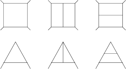
Refer to caption
Figure 3: Relation between integrals of the four-point amplitude (first line) and Wilson line integrals (second line) at one and two loops.
Refer to caption
Refer to caption
Figure 4: Relation between integrals of the four-point amplitude (first and third line) and Wilson line integrals (second and fourth line) at three loops. Arrows denote internal numerator factors (pμ+qμ)2(p^{\mu}+q^{\mu})^{2}, where pμp^{\mu} and qμq^{\mu} are the momenta flowing along the lines with arrows.

In Figs. 3 and 4 we illustrate the relation between the integrals contributing to the four-particle scattering amplitude (odd lines) and the integrals contributing to the cusp anomalous dimension (even lines) to three loops. The integrals occurring at one and two loops are shown in Fig. 3. The three-loop integrals are shown in Fig. 4. The reason for this relation [11, 10] is essentially exact dual conformal symmetry [15], together with the fact that massive scattering amplitudes in soft limits are related to Wilson loops [34].

Appendix D The six-loop function Ω0(6)\Omega_{0}^{(6)}

Here we present the six-loop result Ω0(6)\Omega_{0}^{(6)} which we relegated from the main text to this Appendix. Again, all HPLs are understood to have argument x2x^{2}.

Ω0(6)​(x)=\displaystyle\Omega_{0}^{(6)}(x)= 2563​ζ2​ζ33+160​ζ32​ζ5+612​ζ5​ζ6+432​ζ4​ζ7+24803​ζ3​ζ8+6803​ζ2​ζ9+372​ζ11\displaystyle\;\frac{256}{3}\,\zeta_{2}\,\zeta_{3}^{3}+160\,\zeta_{3}^{2}\,\zeta_{5}+612\,\zeta_{5}\,\zeta_{6}+432\,\zeta_{4}\,\zeta_{7}+\frac{2480}{3}\,\zeta_{3}\,\zeta_{8}+\frac{680}{3}\,\zeta_{2}\,\zeta_{9}+372\,\zeta_{11}
+912​ζ32​ζ4​H0+576​ζ2​ζ3​ζ5​H0+168​ζ52​H0+336​ζ3​ζ7​H0+41465​ζ10​H0\displaystyle+912\,\zeta_{3}^{2}\,\zeta_{4}\,H_{0}+576\,\zeta_{2}\,\zeta_{3}\,\zeta_{5}\,H_{0}+168\,\zeta_{5}^{2}\,H_{0}+336\,\zeta_{3}\,\zeta_{7}\,H_{0}+\frac{4146}{5}\,\zeta_{10}\,H_{0}
+3203​ζ33​H2+1440​ζ4​ζ5​H2+2040​ζ3​ζ6​H2+720​ζ2​ζ7​H2+34003​ζ9​H2\displaystyle+\frac{320}{3}\,\zeta_{3}^{3}\,H_{2}+1440\,\zeta_{4}\,\zeta_{5}\,H_{2}+2040\,\zeta_{3}\,\zeta_{6}\,H_{2}+720\,\zeta_{2}\,\zeta_{7}\,H_{2}+\frac{3400}{3}\,\zeta_{9}\,H_{2}
+1024​ζ2​ζ32​H3+1280​ζ3​ζ5​H3+99203​ζ8​H3+9744​ζ3​ζ4​H4+3360​ζ2​ζ5​H4\displaystyle+1024\,\zeta_{2}\,\zeta_{3}^{2}\,H_{3}+1280\,\zeta_{3}\,\zeta_{5}\,H_{3}+\frac{9920}{3}\,\zeta_{8}\,H_{3}+9744\,\zeta_{3}\,\zeta_{4}\,H_{4}+3360\,\zeta_{2}\,\zeta_{5}\,H_{4}
+2664​ζ7​H4+2176​ζ32​H5+20472​ζ6​H5+14688​ζ2​ζ3​H6+8592​ζ5​H6\displaystyle+2664\,\zeta_{7}\,H_{4}+2176\,\zeta_{3}^{2}\,H_{5}+20472\,\zeta_{6}\,H_{5}+14688\,\zeta_{2}\,\zeta_{3}\,H_{6}+8592\,\zeta_{5}\,H_{6}
+55776​ζ4​H7+31936​ζ3​H8+52928​ζ2​H9+64​ζ33​H0,0+1896​ζ4​ζ5​H0,0\displaystyle+55776\,\zeta_{4}\,H_{7}+31936\,\zeta_{3}\,H_{8}+52928\,\zeta_{2}\,H_{9}+64\,\zeta_{3}^{3}\,H_{0,0}+1896\,\zeta_{4}\,\zeta_{5}\,H_{0,0}
+3792​ζ3​ζ6​H0,0+576​ζ2​ζ7​H0,0+332​ζ9​H0,0+640​ζ2​ζ32​H2,0+800​ζ3​ζ5​H2,0\displaystyle+3792\,\zeta_{3}\,\zeta_{6}\,H_{0,0}+576\,\zeta_{2}\,\zeta_{7}\,H_{0,0}+332\,\zeta_{9}\,H_{0,0}+640\,\zeta_{2}\,\zeta_{3}^{2}\,H_{2,0}+800\,\zeta_{3}\,\zeta_{5}\,H_{2,0}
+62003​ζ8​H2,0+3840​ζ3​ζ4​H2,2+1920​ζ2​ζ5​H2,2+2880​ζ7​H2,2+960​ζ32​H2,3\displaystyle+\frac{6200}{3}\,\zeta_{8}\,H_{2,0}+3840\,\zeta_{3}\,\zeta_{4}\,H_{2,2}+1920\,\zeta_{2}\,\zeta_{5}\,H_{2,2}+2880\,\zeta_{7}\,H_{2,2}+960\,\zeta_{3}^{2}\,H_{2,3}
+6120​ζ6​H2,3+5760​ζ2​ζ3​H2,4+5280​ζ5​H2,4+17760​ζ4​H2,5+12160​ζ3​H2,6\displaystyle+6120\,\zeta_{6}\,H_{2,3}+5760\,\zeta_{2}\,\zeta_{3}\,H_{2,4}+5280\,\zeta_{5}\,H_{2,4}+17760\,\zeta_{4}\,H_{2,5}+12160\,\zeta_{3}\,H_{2,6}
+15680​ζ2​H2,7+7296​ζ3​ζ4​H3,0+2304​ζ2​ζ5​H3,0+1344​ζ7​H3,0+6144​ζ3​ζ4​H3,1\displaystyle+15680\,\zeta_{2}\,H_{2,7}+7296\,\zeta_{3}\,\zeta_{4}\,H_{3,0}+2304\,\zeta_{2}\,\zeta_{5}\,H_{3,0}+1344\,\zeta_{7}\,H_{3,0}+6144\,\zeta_{3}\,\zeta_{4}\,H_{3,1}
+3072​ζ2​ζ5​H3,1+4608​ζ7​H3,1+1536​ζ32​H3,2+9792​ζ6​H3,2+9216​ζ2​ζ3​H3,3\displaystyle+3072\,\zeta_{2}\,\zeta_{5}\,H_{3,1}+4608\,\zeta_{7}\,H_{3,1}+1536\,\zeta_{3}^{2}\,H_{3,2}+9792\,\zeta_{6}\,H_{3,2}+9216\,\zeta_{2}\,\zeta_{3}\,H_{3,3}
+8448​ζ5​H3,3+28416​ζ4​H3,4+19456​ζ3​H3,5+25088​ζ2​H3,6+1280​ζ32​H4,0\displaystyle+8448\,\zeta_{5}\,H_{3,3}+28416\,\zeta_{4}\,H_{3,4}+19456\,\zeta_{3}\,H_{3,5}+25088\,\zeta_{2}\,H_{3,6}+1280\,\zeta_{3}^{2}\,H_{4,0}
+18696​ζ6​H4,0+1728​ζ32​H4,1+11016​ζ6​H4,1+11904​ζ2​ζ3​H4,2+11808​ζ5​H4,2\displaystyle+18696\,\zeta_{6}\,H_{4,0}+1728\,\zeta_{3}^{2}\,H_{4,1}+11016\,\zeta_{6}\,H_{4,1}+11904\,\zeta_{2}\,\zeta_{3}\,H_{4,2}+11808\,\zeta_{5}\,H_{4,2}
+35040​ζ4​H4,3+25664​ζ3​H4,4+31744​ζ2​H4,5+10944​ζ2​ζ3​H5,0+5376​ζ5​H5,0\displaystyle+35040\,\zeta_{4}\,H_{4,3}+25664\,\zeta_{3}\,H_{4,4}+31744\,\zeta_{2}\,H_{4,5}+10944\,\zeta_{2}\,\zeta_{3}\,H_{5,0}+5376\,\zeta_{5}\,H_{5,0}
+14208​ζ2​ζ3​H5,1+15936​ζ5​H5,1+38400​ζ4​H5,2+32064​ζ3​H5,3+36864​ζ2​H5,4\displaystyle+14208\,\zeta_{2}\,\zeta_{3}\,H_{5,1}+15936\,\zeta_{5}\,H_{5,1}+38400\,\zeta_{4}\,H_{5,2}+32064\,\zeta_{3}\,H_{5,3}+36864\,\zeta_{2}\,H_{5,4}
+56232​ζ4​H6,0+36960​ζ4​H6,1+38976​ζ3​H6,2+40128​ζ2​H6,3+22400​ζ3​H7,0\displaystyle+56232\,\zeta_{4}\,H_{6,0}+36960\,\zeta_{4}\,H_{6,1}+38976\,\zeta_{3}\,H_{6,2}+40128\,\zeta_{2}\,H_{6,3}+22400\,\zeta_{3}\,H_{7,0}
+45248​ζ3​H7,1+39424​ζ2​H7,2+67712​ζ2​H8,0+29568​ζ2​H8,1+84752​H10,0\displaystyle+45248\,\zeta_{3}\,H_{7,1}+39424\,\zeta_{2}\,H_{7,2}+67712\,\zeta_{2}\,H_{8,0}+29568\,\zeta_{2}\,H_{8,1}+84752\,H_{10,0}
+736​ζ2​ζ32​H0,0,0+608​ζ3​ζ5​H0,0,0+200123​ζ8​H0,0,0+4560​ζ3​ζ4​H2,0,0\displaystyle+736\,\zeta_{2}\,\zeta_{3}^{2}\,H_{0,0,0}+608\,\zeta_{3}\,\zeta_{5}\,H_{0,0,0}+\frac{20012}{3}\,\zeta_{8}\,H_{0,0,0}+4560\,\zeta_{3}\,\zeta_{4}\,H_{2,0,0}
+1440​ζ2​ζ5​H2,0,0+840​ζ7​H2,0,0+640​ζ32​H2,2,0+4080​ζ6​H2,2,0+3840​ζ2​ζ3​H2,2,2\displaystyle+1440\,\zeta_{2}\,\zeta_{5}\,H_{2,0,0}+840\,\zeta_{7}\,H_{2,0,0}+640\,\zeta_{3}^{2}\,H_{2,2,0}+4080\,\zeta_{6}\,H_{2,2,0}+3840\,\zeta_{2}\,\zeta_{3}\,H_{2,2,2}
+5760​ζ5​H2,2,2+7680​ζ4​H2,2,3+7040​ζ3​H2,2,4+6400​ζ2​H2,2,5+3840​ζ2​ζ3​H2,3,0\displaystyle+5760\,\zeta_{5}\,H_{2,2,2}+7680\,\zeta_{4}\,H_{2,2,3}+7040\,\zeta_{3}\,H_{2,2,4}+6400\,\zeta_{2}\,H_{2,2,5}+3840\,\zeta_{2}\,\zeta_{3}\,H_{2,3,0}
+2400​ζ5​H2,3,0+5760​ζ2​ζ3​H2,3,1+8640​ζ5​H2,3,1+11520​ζ4​H2,3,2\displaystyle+2400\,\zeta_{5}\,H_{2,3,0}+5760\,\zeta_{2}\,\zeta_{3}\,H_{2,3,1}+8640\,\zeta_{5}\,H_{2,3,1}+11520\,\zeta_{4}\,H_{2,3,2}
+10560​ζ3​H2,3,3+9600​ζ2​H2,3,4+16560​ζ4​H2,4,0+11520​ζ4​H2,4,1\displaystyle+10560\,\zeta_{3}\,H_{2,3,3}+9600\,\zeta_{2}\,H_{2,3,4}+16560\,\zeta_{4}\,H_{2,4,0}+11520\,\zeta_{4}\,H_{2,4,1}
+14400​ζ3​H2,4,2+11520​ζ2​H2,4,3+7040​ζ3​H2,5,0+18560​ζ3​H2,5,1\displaystyle+14400\,\zeta_{3}\,H_{2,4,2}+11520\,\zeta_{2}\,H_{2,4,3}+7040\,\zeta_{3}\,H_{2,5,0}+18560\,\zeta_{3}\,H_{2,5,1}
+12160​ζ2​H2,5,2+18080​ζ2​H2,6,0+9600​ζ2​H2,6,1+21440​H2,8,0\displaystyle+12160\,\zeta_{2}\,H_{2,5,2}+18080\,\zeta_{2}\,H_{2,6,0}+9600\,\zeta_{2}\,H_{2,6,1}+21440\,H_{2,8,0}
+768​ζ32​H3,0,0+15168​ζ6​H3,0,0+1024​ζ32​H3,1,0+6528​ζ6​H3,1,0\displaystyle+768\,\zeta_{3}^{2}\,H_{3,0,0}+15168\,\zeta_{6}\,H_{3,0,0}+1024\,\zeta_{3}^{2}\,H_{3,1,0}+6528\,\zeta_{6}\,H_{3,1,0}
+6144​ζ2​ζ3​H3,1,2+9216​ζ5​H3,1,2+12288​ζ4​H3,1,3+11264​ζ3​H3,1,4\displaystyle+6144\,\zeta_{2}\,\zeta_{3}\,H_{3,1,2}+9216\,\zeta_{5}\,H_{3,1,2}+12288\,\zeta_{4}\,H_{3,1,3}+11264\,\zeta_{3}\,H_{3,1,4}
+10240​ζ2​H3,1,5+6144​ζ2​ζ3​H3,2,0+3840​ζ5​H3,2,0+9216​ζ2​ζ3​H3,2,1\displaystyle+10240\,\zeta_{2}\,H_{3,1,5}+6144\,\zeta_{2}\,\zeta_{3}\,H_{3,2,0}+3840\,\zeta_{5}\,H_{3,2,0}+9216\,\zeta_{2}\,\zeta_{3}\,H_{3,2,1}
+13824​ζ5​H3,2,1+18432​ζ4​H3,2,2+16896​ζ3​H3,2,3+15360​ζ2​H3,2,4\displaystyle+13824\,\zeta_{5}\,H_{3,2,1}+18432\,\zeta_{4}\,H_{3,2,2}+16896\,\zeta_{3}\,H_{3,2,3}+15360\,\zeta_{2}\,H_{3,2,4}
+26496​ζ4​H3,3,0+18432​ζ4​H3,3,1+23040​ζ3​H3,3,2+18432​ζ2​H3,3,3\displaystyle+26496\,\zeta_{4}\,H_{3,3,0}+18432\,\zeta_{4}\,H_{3,3,1}+23040\,\zeta_{3}\,H_{3,3,2}+18432\,\zeta_{2}\,H_{3,3,3}
+11264​ζ3​H3,4,0+29696​ζ3​H3,4,1+19456​ζ2​H3,4,2+28928​ζ2​H3,5,0\displaystyle+11264\,\zeta_{3}\,H_{3,4,0}+29696\,\zeta_{3}\,H_{3,4,1}+19456\,\zeta_{2}\,H_{3,4,2}+28928\,\zeta_{2}\,H_{3,5,0}
+15360​ζ2​H3,5,1+34304​H3,7,0+8128​ζ2​ζ3​H4,0,0+3616​ζ5​H4,0,0\displaystyle+15360\,\zeta_{2}\,H_{3,5,1}+34304\,H_{3,7,0}+8128\,\zeta_{2}\,\zeta_{3}\,H_{4,0,0}+3616\,\zeta_{5}\,H_{4,0,0}
+6912​ζ2​ζ3​H4,1,0+4320​ζ5​H4,1,0+10368​ζ2​ζ3​H4,1,1+15552​ζ5​H4,1,1\displaystyle+6912\,\zeta_{2}\,\zeta_{3}\,H_{4,1,0}+4320\,\zeta_{5}\,H_{4,1,0}+10368\,\zeta_{2}\,\zeta_{3}\,H_{4,1,1}+15552\,\zeta_{5}\,H_{4,1,1}
+20736​ζ4​H4,1,2+19008​ζ3​H4,1,3+17280​ζ2​H4,1,4+32112​ζ4​H4,2,0\displaystyle+20736\,\zeta_{4}\,H_{4,1,2}+19008\,\zeta_{3}\,H_{4,1,3}+17280\,\zeta_{2}\,H_{4,1,4}+32112\,\zeta_{4}\,H_{4,2,0}
+20736​ζ4​H4,2,1+28992​ζ3​H4,2,2+22272​ζ2​H4,2,3+14656​ζ3​H4,3,0\displaystyle+20736\,\zeta_{4}\,H_{4,2,1}+28992\,\zeta_{3}\,H_{4,2,2}+22272\,\zeta_{2}\,H_{4,2,3}+14656\,\zeta_{3}\,H_{4,3,0}
+37504​ζ3​H4,3,1+23936​ζ2​H4,3,2+36544​ζ2​H4,4,0+18816​ζ2​H4,4,1\displaystyle+37504\,\zeta_{3}\,H_{4,3,1}+23936\,\zeta_{2}\,H_{4,3,2}+36544\,\zeta_{2}\,H_{4,4,0}+18816\,\zeta_{2}\,H_{4,4,1}
+43936​H4,6,0+51360​ζ4​H5,0,0+33984​ζ4​H5,1,0+18432​ζ4​H5,1,1\displaystyle+43936\,H_{4,6,0}+51360\,\zeta_{4}\,H_{5,0,0}+33984\,\zeta_{4}\,H_{5,1,0}+18432\,\zeta_{4}\,H_{5,1,1}
+33024​ζ3​H5,1,2+23424​ζ2​H5,1,3+18048​ζ3​H5,2,0+43008​ζ3​H5,2,1\displaystyle+33024\,\zeta_{3}\,H_{5,1,2}+23424\,\zeta_{2}\,H_{5,1,3}+18048\,\zeta_{3}\,H_{5,2,0}+43008\,\zeta_{3}\,H_{5,2,1}
+26112​ζ2​H5,2,2+42432​ζ2​H5,3,0+20352​ζ2​H5,3,1+52512​H5,5,0\displaystyle+26112\,\zeta_{2}\,H_{5,2,2}+42432\,\zeta_{2}\,H_{5,3,0}+20352\,\zeta_{2}\,H_{5,3,1}+52512\,H_{5,5,0}
+15776​ζ3​H6,0,0+21120​ζ3​H6,1,0+44160​ζ3​H6,1,1+24960​ζ2​H6,1,2\displaystyle+15776\,\zeta_{3}\,H_{6,0,0}+21120\,\zeta_{3}\,H_{6,1,0}+44160\,\zeta_{3}\,H_{6,1,1}+24960\,\zeta_{2}\,H_{6,1,2}
+46368​ζ2​H6,2,0+19200​ζ2​H6,2,1+60576​H6,4,0+66976​ζ2​H7,0,0\displaystyle+46368\,\zeta_{2}\,H_{6,2,0}+19200\,\zeta_{2}\,H_{6,2,1}+60576\,H_{6,4,0}+66976\,\zeta_{2}\,H_{7,0,0}
+46144​ζ2​H7,1,0+13440​ζ2​H7,1,1+66976​H7,3,0+67712​H8,2,0\displaystyle+46144\,\zeta_{2}\,H_{7,1,0}+13440\,\zeta_{2}\,H_{7,1,1}+66976\,H_{7,3,0}+67712\,H_{8,2,0}
+105856​H9,0,0+52928​H9,1,0+8688​ζ3​ζ4​H0,0,0,0+2064​ζ2​ζ5​H0,0,0,0\displaystyle+105856\,H_{9,0,0}+52928\,H_{9,1,0}+8688\,\zeta_{3}\,\zeta_{4}\,H_{0,0,0,0}+2064\,\zeta_{2}\,\zeta_{5}\,H_{0,0,0,0}
+792​ζ7​H0,0,0,0+480​ζ32​H2,0,0,0+9480​ζ6​H2,0,0,0+2560​ζ2​ζ3​H2,2,0,0\displaystyle+792\,\zeta_{7}\,H_{0,0,0,0}+480\,\zeta_{3}^{2}\,H_{2,0,0,0}+9480\,\zeta_{6}\,H_{2,0,0,0}+2560\,\zeta_{2}\,\zeta_{3}\,H_{2,2,0,0}
+1600​ζ5​H2,2,0,0+5760​ζ4​H2,2,2,0+7680​ζ3​H2,2,2,2+3840​ζ2​H2,2,2,3\displaystyle+1600\,\zeta_{5}\,H_{2,2,0,0}+5760\,\zeta_{4}\,H_{2,2,2,0}+7680\,\zeta_{3}\,H_{2,2,2,2}+3840\,\zeta_{2}\,H_{2,2,2,3}
+2560​ζ3​H2,2,3,0+10240​ζ3​H2,2,3,1+5120​ζ2​H2,2,3,2+6400​ζ2​H2,2,4,0\displaystyle+2560\,\zeta_{3}\,H_{2,2,3,0}+10240\,\zeta_{3}\,H_{2,2,3,1}+5120\,\zeta_{2}\,H_{2,2,3,2}+6400\,\zeta_{2}\,H_{2,2,4,0}
+3840​ζ2​H2,2,4,1+7360​H2,2,6,0+13680​ζ4​H2,3,0,0+8640​ζ4​H2,3,1,0\displaystyle+3840\,\zeta_{2}\,H_{2,2,4,1}+7360\,H_{2,2,6,0}+13680\,\zeta_{4}\,H_{2,3,0,0}+8640\,\zeta_{4}\,H_{2,3,1,0}
+11520​ζ3​H2,3,1,2+5760​ζ2​H2,3,1,3+3840​ζ3​H2,3,2,0+15360​ζ3​H2,3,2,1\displaystyle+11520\,\zeta_{3}\,H_{2,3,1,2}+5760\,\zeta_{2}\,H_{2,3,1,3}+3840\,\zeta_{3}\,H_{2,3,2,0}+15360\,\zeta_{3}\,H_{2,3,2,1}
+7680​ζ2​H2,3,2,2+9600​ζ2​H2,3,3,0+5760​ζ2​H2,3,3,1+11040​H2,3,5,0\displaystyle+7680\,\zeta_{2}\,H_{2,3,2,2}+9600\,\zeta_{2}\,H_{2,3,3,0}+5760\,\zeta_{2}\,H_{2,3,3,1}+11040\,H_{2,3,5,0}
+4480​ζ3​H2,4,0,0+3840​ζ3​H2,4,1,0+15360​ζ3​H2,4,1,1+7680​ζ2​H2,4,1,2\displaystyle+4480\,\zeta_{3}\,H_{2,4,0,0}+3840\,\zeta_{3}\,H_{2,4,1,0}+15360\,\zeta_{3}\,H_{2,4,1,1}+7680\,\zeta_{2}\,H_{2,4,1,2}
+11520​ζ2​H2,4,2,0+5760​ζ2​H2,4,2,1+13920​H2,4,4,0+16480​ζ2​H2,5,0,0\displaystyle+11520\,\zeta_{2}\,H_{2,4,2,0}+5760\,\zeta_{2}\,H_{2,4,2,1}+13920\,H_{2,4,4,0}+16480\,\zeta_{2}\,H_{2,5,0,0}
+12160​ζ2​H2,5,1,0+3840​ζ2​H2,5,1,1+16480​H2,5,3,0+18080​H2,6,2,0\displaystyle+12160\,\zeta_{2}\,H_{2,5,1,0}+3840\,\zeta_{2}\,H_{2,5,1,1}+16480\,H_{2,5,3,0}+18080\,H_{2,6,2,0}
+23520​H2,7,0,0+15680​H2,7,1,0+5888​ζ2​ζ3​H3,0,0,0+2432​ζ5​H3,0,0,0\displaystyle+23520\,H_{2,7,0,0}+15680\,H_{2,7,1,0}+5888\,\zeta_{2}\,\zeta_{3}\,H_{3,0,0,0}+2432\,\zeta_{5}\,H_{3,0,0,0}
+4096​ζ2​ζ3​H3,1,0,0+2560​ζ5​H3,1,0,0+9216​ζ4​H3,1,2,0+12288​ζ3​H3,1,2,2\displaystyle+4096\,\zeta_{2}\,\zeta_{3}\,H_{3,1,0,0}+2560\,\zeta_{5}\,H_{3,1,0,0}+9216\,\zeta_{4}\,H_{3,1,2,0}+12288\,\zeta_{3}\,H_{3,1,2,2}
+6144​ζ2​H3,1,2,3+4096​ζ3​H3,1,3,0+16384​ζ3​H3,1,3,1+8192​ζ2​H3,1,3,2\displaystyle+6144\,\zeta_{2}\,H_{3,1,2,3}+4096\,\zeta_{3}\,H_{3,1,3,0}+16384\,\zeta_{3}\,H_{3,1,3,1}+8192\,\zeta_{2}\,H_{3,1,3,2}
+10240​ζ2​H3,1,4,0+6144​ζ2​H3,1,4,1+11776​H3,1,6,0+21888​ζ4​H3,2,0,0\displaystyle+10240\,\zeta_{2}\,H_{3,1,4,0}+6144\,\zeta_{2}\,H_{3,1,4,1}+11776\,H_{3,1,6,0}+21888\,\zeta_{4}\,H_{3,2,0,0}
+13824​ζ4​H3,2,1,0+18432​ζ3​H3,2,1,2+9216​ζ2​H3,2,1,3+6144​ζ3​H3,2,2,0\displaystyle+13824\,\zeta_{4}\,H_{3,2,1,0}+18432\,\zeta_{3}\,H_{3,2,1,2}+9216\,\zeta_{2}\,H_{3,2,1,3}+6144\,\zeta_{3}\,H_{3,2,2,0}
+24576​ζ3​H3,2,2,1+12288​ζ2​H3,2,2,2+15360​ζ2​H3,2,3,0+9216​ζ2​H3,2,3,1\displaystyle+24576\,\zeta_{3}\,H_{3,2,2,1}+12288\,\zeta_{2}\,H_{3,2,2,2}+15360\,\zeta_{2}\,H_{3,2,3,0}+9216\,\zeta_{2}\,H_{3,2,3,1}
+17664​H3,2,5,0+7168​ζ3​H3,3,0,0+6144​ζ3​H3,3,1,0+24576​ζ3​H3,3,1,1\displaystyle+17664\,H_{3,2,5,0}+7168\,\zeta_{3}\,H_{3,3,0,0}+6144\,\zeta_{3}\,H_{3,3,1,0}+24576\,\zeta_{3}\,H_{3,3,1,1}
+12288​ζ2​H3,3,1,2+18432​ζ2​H3,3,2,0+9216​ζ2​H3,3,2,1+22272​H3,3,4,0\displaystyle+12288\,\zeta_{2}\,H_{3,3,1,2}+18432\,\zeta_{2}\,H_{3,3,2,0}+9216\,\zeta_{2}\,H_{3,3,2,1}+22272\,H_{3,3,4,0}
+26368​ζ2​H3,4,0,0+19456​ζ2​H3,4,1,0+6144​ζ2​H3,4,1,1+26368​H3,4,3,0\displaystyle+26368\,\zeta_{2}\,H_{3,4,0,0}+19456\,\zeta_{2}\,H_{3,4,1,0}+6144\,\zeta_{2}\,H_{3,4,1,1}+26368\,H_{3,4,3,0}
+28928​H3,5,2,0+37632​H3,6,0,0+25088​H3,6,1,0+44064​ζ4​H4,0,0,0\displaystyle+28928\,H_{3,5,2,0}+37632\,H_{3,6,0,0}+25088\,H_{3,6,1,0}+44064\,\zeta_{4}\,H_{4,0,0,0}
+24624​ζ4​H4,1,0,0+15552​ζ4​H4,1,1,0+20736​ζ3​H4,1,1,2+10368​ζ2​H4,1,1,3\displaystyle+24624\,\zeta_{4}\,H_{4,1,0,0}+15552\,\zeta_{4}\,H_{4,1,1,0}+20736\,\zeta_{3}\,H_{4,1,1,2}+10368\,\zeta_{2}\,H_{4,1,1,3}
+6912​ζ3​H4,1,2,0+27648​ζ3​H4,1,2,1+13824​ζ2​H4,1,2,2+17280​ζ2​H4,1,3,0\displaystyle+6912\,\zeta_{3}\,H_{4,1,2,0}+27648\,\zeta_{3}\,H_{4,1,2,1}+13824\,\zeta_{2}\,H_{4,1,2,2}+17280\,\zeta_{2}\,H_{4,1,3,0}
+10368​ζ2​H4,1,3,1+19872​H4,1,5,0+9472​ζ3​H4,2,0,0+6912​ζ3​H4,2,1,0\displaystyle+10368\,\zeta_{2}\,H_{4,1,3,1}+19872\,H_{4,1,5,0}+9472\,\zeta_{3}\,H_{4,2,0,0}+6912\,\zeta_{3}\,H_{4,2,1,0}
+27648​ζ3​H4,2,1,1+13824​ζ2​H4,2,1,2+22272​ζ2​H4,2,2,0+10368​ζ2​H4,2,2,1\displaystyle+27648\,\zeta_{3}\,H_{4,2,1,1}+13824\,\zeta_{2}\,H_{4,2,1,2}+22272\,\zeta_{2}\,H_{4,2,2,0}+10368\,\zeta_{2}\,H_{4,2,2,1}
+27552​H4,2,4,0+33152​ζ2​H4,3,0,0+23936​ζ2​H4,3,1,0+6912​ζ2​H4,3,1,1\displaystyle+27552\,H_{4,2,4,0}+33152\,\zeta_{2}\,H_{4,3,0,0}+23936\,\zeta_{2}\,H_{4,3,1,0}+6912\,\zeta_{2}\,H_{4,3,1,1}
+33152​H4,3,3,0+36544​H4,4,2,0+47936​H4,5,0,0+31744​H4,5,1,0\displaystyle+33152\,H_{4,3,3,0}+36544\,H_{4,4,2,0}+47936\,H_{4,5,0,0}+31744\,H_{4,5,1,0}
+11264​ζ3​H5,0,0,0+11968​ζ3​H5,1,0,0+6144​ζ3​H5,1,1,0+24576​ζ3​H5,1,1,1\displaystyle+11264\,\zeta_{3}\,H_{5,0,0,0}+11968\,\zeta_{3}\,H_{5,1,0,0}+6144\,\zeta_{3}\,H_{5,1,1,0}+24576\,\zeta_{3}\,H_{5,1,1,1}
+12288​ζ2​H5,1,1,2+23424​ζ2​H5,1,2,0+9216​ζ2​H5,1,2,1+30720​H5,1,4,0\displaystyle+12288\,\zeta_{2}\,H_{5,1,1,2}+23424\,\zeta_{2}\,H_{5,1,2,0}+9216\,\zeta_{2}\,H_{5,1,2,1}+30720\,H_{5,1,4,0}
+38208​ζ2​H5,2,0,0+26112​ζ2​H5,2,1,0+6144​ζ2​H5,2,1,1+38208​H5,2,3,0\displaystyle+38208\,\zeta_{2}\,H_{5,2,0,0}+26112\,\zeta_{2}\,H_{5,2,1,0}+6144\,\zeta_{2}\,H_{5,2,1,1}+38208\,H_{5,2,3,0}
+42432​H5,3,2,0+56896​H5,4,0,0+36864​H5,4,1,0+60576​ζ2​H6,0,0,0\displaystyle+42432\,H_{5,3,2,0}+56896\,H_{5,4,0,0}+36864\,H_{5,4,1,0}+60576\,\zeta_{2}\,H_{6,0,0,0}
+40800​ζ2​H6,1,0,0+24960​ζ2​H6,1,1,0+3840​ζ2​H6,1,1,1+40800​H6,1,3,0\displaystyle+40800\,\zeta_{2}\,H_{6,1,0,0}+24960\,\zeta_{2}\,H_{6,1,1,0}+3840\,\zeta_{2}\,H_{6,1,1,1}+40800\,H_{6,1,3,0}
+46368​H6,2,2,0+65248​H6,3,0,0+40128​H6,3,1,0+46144​H7,1,2,0\displaystyle+46368\,H_{6,2,2,0}+65248\,H_{6,3,0,0}+40128\,H_{6,3,1,0}+46144\,H_{7,1,2,0}
+72128​H7,2,0,0+39424​H7,2,1,0+102640​H8,0,0,0+73920​H8,1,0,0\displaystyle+72128\,H_{7,2,0,0}+39424\,H_{7,2,1,0}+102640\,H_{8,0,0,0}+73920\,H_{8,1,0,0}
+29568​H8,1,1,0+736​ζ32​H0,0,0,0,0+27736​ζ6​H0,0,0,0,0+3680​ζ2​ζ3​H2,0,0,0,0\displaystyle+29568\,H_{8,1,1,0}+736\,\zeta_{3}^{2}\,H_{0,0,0,0,0}+27736\,\zeta_{6}\,H_{0,0,0,0,0}+3680\,\zeta_{2}\,\zeta_{3}\,H_{2,0,0,0,0}
+1520​ζ5​H2,0,0,0,0+9120​ζ4​H2,2,0,0,0+1920​ζ3​H2,2,2,0,0+3840​ζ2​H2,2,2,2,0\displaystyle+1520\,\zeta_{5}\,H_{2,0,0,0,0}+9120\,\zeta_{4}\,H_{2,2,0,0,0}+1920\,\zeta_{3}\,H_{2,2,2,0,0}+3840\,\zeta_{2}\,H_{2,2,2,2,0}
+3840​H2,2,2,4,0+5120​ζ2​H2,2,3,0,0+5120​ζ2​H2,2,3,1,0+5120​H2,2,3,3,0\displaystyle+3840\,H_{2,2,2,4,0}+5120\,\zeta_{2}\,H_{2,2,3,0,0}+5120\,\zeta_{2}\,H_{2,2,3,1,0}+5120\,H_{2,2,3,3,0}
+6400​H2,2,4,2,0+6400​H2,2,5,0,0+6400​H2,2,5,1,0+2880​ζ3​H2,3,0,0,0\displaystyle+6400\,H_{2,2,4,2,0}+6400\,H_{2,2,5,0,0}+6400\,H_{2,2,5,1,0}+2880\,\zeta_{3}\,H_{2,3,0,0,0}
+2880​ζ3​H2,3,1,0,0+5760​ζ2​H2,3,1,2,0+5760​H2,3,1,4,0+7680​ζ2​H2,3,2,0,0\displaystyle+2880\,\zeta_{3}\,H_{2,3,1,0,0}+5760\,\zeta_{2}\,H_{2,3,1,2,0}+5760\,H_{2,3,1,4,0}+7680\,\zeta_{2}\,H_{2,3,2,0,0}
+7680​ζ2​H2,3,2,1,0+7680​H2,3,2,3,0+9600​H2,3,3,2,0+9600​H2,3,4,0,0\displaystyle+7680\,\zeta_{2}\,H_{2,3,2,1,0}+7680\,H_{2,3,2,3,0}+9600\,H_{2,3,3,2,0}+9600\,H_{2,3,4,0,0}
+9600​H2,3,4,1,0+13920​ζ2​H2,4,0,0,0+7680​ζ2​H2,4,1,0,0+7680​ζ2​H2,4,1,1,0\displaystyle+9600\,H_{2,3,4,1,0}+13920\,\zeta_{2}\,H_{2,4,0,0,0}+7680\,\zeta_{2}\,H_{2,4,1,0,0}+7680\,\zeta_{2}\,H_{2,4,1,1,0}
+7680​H2,4,1,3,0+11520​H2,4,2,2,0+11840​H2,4,3,0,0+11520​H2,4,3,1,0\displaystyle+7680\,H_{2,4,1,3,0}+11520\,H_{2,4,2,2,0}+11840\,H_{2,4,3,0,0}+11520\,H_{2,4,3,1,0}
+12160​H2,5,1,2,0+13760​H2,5,2,0,0+12160​H2,5,2,1,0+20800​H2,6,0,0,0\displaystyle+12160\,H_{2,5,1,2,0}+13760\,H_{2,5,2,0,0}+12160\,H_{2,5,2,1,0}+20800\,H_{2,6,0,0,0}
+14400​H2,6,1,0,0+9600​H2,6,1,1,0+34752​ζ4​H3,0,0,0,0+14592​ζ4​H3,1,0,0,0\displaystyle+14400\,H_{2,6,1,0,0}+9600\,H_{2,6,1,1,0}+34752\,\zeta_{4}\,H_{3,0,0,0,0}+14592\,\zeta_{4}\,H_{3,1,0,0,0}
+3072​ζ3​H3,1,2,0,0+6144​ζ2​H3,1,2,2,0+6144​H3,1,2,4,0+8192​ζ2​H3,1,3,0,0\displaystyle+3072\,\zeta_{3}\,H_{3,1,2,0,0}+6144\,\zeta_{2}\,H_{3,1,2,2,0}+6144\,H_{3,1,2,4,0}+8192\,\zeta_{2}\,H_{3,1,3,0,0}
+8192​ζ2​H3,1,3,1,0+8192​H3,1,3,3,0+10240​H3,1,4,2,0+10240​H3,1,5,0,0\displaystyle+8192\,\zeta_{2}\,H_{3,1,3,1,0}+8192\,H_{3,1,3,3,0}+10240\,H_{3,1,4,2,0}+10240\,H_{3,1,5,0,0}
+10240​H3,1,5,1,0+4608​ζ3​H3,2,0,0,0+4608​ζ3​H3,2,1,0,0+9216​ζ2​H3,2,1,2,0\displaystyle+10240\,H_{3,1,5,1,0}+4608\,\zeta_{3}\,H_{3,2,0,0,0}+4608\,\zeta_{3}\,H_{3,2,1,0,0}+9216\,\zeta_{2}\,H_{3,2,1,2,0}
+9216​H3,2,1,4,0+12288​ζ2​H3,2,2,0,0+12288​ζ2​H3,2,2,1,0+12288​H3,2,2,3,0\displaystyle+9216\,H_{3,2,1,4,0}+12288\,\zeta_{2}\,H_{3,2,2,0,0}+12288\,\zeta_{2}\,H_{3,2,2,1,0}+12288\,H_{3,2,2,3,0}
+15360​H3,2,3,2,0+15360​H3,2,4,0,0+15360​H3,2,4,1,0+22272​ζ2​H3,3,0,0,0\displaystyle+15360\,H_{3,2,3,2,0}+15360\,H_{3,2,4,0,0}+15360\,H_{3,2,4,1,0}+22272\,\zeta_{2}\,H_{3,3,0,0,0}
+12288​ζ2​H3,3,1,0,0+12288​ζ2​H3,3,1,1,0+12288​H3,3,1,3,0+18432​H3,3,2,2,0\displaystyle+12288\,\zeta_{2}\,H_{3,3,1,0,0}+12288\,\zeta_{2}\,H_{3,3,1,1,0}+12288\,H_{3,3,1,3,0}+18432\,H_{3,3,2,2,0}
+18944​H3,3,3,0,0+18432​H3,3,3,1,0+19456​H3,4,1,2,0+22016​H3,4,2,0,0\displaystyle+18944\,H_{3,3,3,0,0}+18432\,H_{3,3,3,1,0}+19456\,H_{3,4,1,2,0}+22016\,H_{3,4,2,0,0}
+19456​H3,4,2,1,0+33280​H3,5,0,0,0+23040​H3,5,1,0,0+15360​H3,5,1,1,0\displaystyle+19456\,H_{3,4,2,1,0}+33280\,H_{3,5,0,0,0}+23040\,H_{3,5,1,0,0}+15360\,H_{3,5,1,1,0}
+8192​ζ3​H4,0,0,0,0+5184​ζ3​H4,1,0,0,0+5184​ζ3​H4,1,1,0,0+10368​ζ2​H4,1,1,2,0\displaystyle+8192\,\zeta_{3}\,H_{4,0,0,0,0}+5184\,\zeta_{3}\,H_{4,1,0,0,0}+5184\,\zeta_{3}\,H_{4,1,1,0,0}+10368\,\zeta_{2}\,H_{4,1,1,2,0}
+10368​H4,1,1,4,0+13824​ζ2​H4,1,2,0,0+13824​ζ2​H4,1,2,1,0+13824​H4,1,2,3,0\displaystyle+10368\,H_{4,1,1,4,0}+13824\,\zeta_{2}\,H_{4,1,2,0,0}+13824\,\zeta_{2}\,H_{4,1,2,1,0}+13824\,H_{4,1,2,3,0}
+17280​H4,1,3,2,0+17280​H4,1,4,0,0+17280​H4,1,4,1,0+27552​ζ2​H4,2,0,0,0\displaystyle+17280\,H_{4,1,3,2,0}+17280\,H_{4,1,4,0,0}+17280\,H_{4,1,4,1,0}+27552\,\zeta_{2}\,H_{4,2,0,0,0}
+13824​ζ2​H4,2,1,0,0+13824​ζ2​H4,2,1,1,0+13824​H4,2,1,3,0+22272​H4,2,2,2,0\displaystyle+13824\,\zeta_{2}\,H_{4,2,1,0,0}+13824\,\zeta_{2}\,H_{4,2,1,1,0}+13824\,H_{4,2,1,3,0}+22272\,H_{4,2,2,2,0}
+23360​H4,2,3,0,0+22272​H4,2,3,1,0+23936​H4,3,1,2,0+27712​H4,3,2,0,0\displaystyle+23360\,H_{4,2,3,0,0}+22272\,H_{4,2,3,1,0}+23936\,H_{4,3,1,2,0}+27712\,H_{4,3,2,0,0}
+23936​H4,3,2,1,0+42368​H4,4,0,0,0+28608​H4,4,1,0,0+18816​H4,4,1,1,0\displaystyle+23936\,H_{4,3,2,1,0}+42368\,H_{4,4,0,0,0}+28608\,H_{4,4,1,0,0}+18816\,H_{4,4,1,1,0}
+52512​ζ2​H5,0,0,0,0+30720​ζ2​H5,1,0,0,0+12288​ζ2​H5,1,1,0,0+12288​ζ2​H5,1,1,1,0\displaystyle+52512\,\zeta_{2}\,H_{5,0,0,0,0}+30720\,\zeta_{2}\,H_{5,1,0,0,0}+12288\,\zeta_{2}\,H_{5,1,1,0,0}+12288\,\zeta_{2}\,H_{5,1,1,1,0}
+12288​H5,1,1,3,0+23424​H5,1,2,2,0+26048​H5,1,3,0,0+23424​H5,1,3,1,0\displaystyle+12288\,H_{5,1,1,3,0}+23424\,H_{5,1,2,2,0}+26048\,H_{5,1,3,0,0}+23424\,H_{5,1,3,1,0}
+26112​H5,2,1,2,0+32256​H5,2,2,0,0+26112​H5,2,2,1,0+50304​H5,3,0,0,0\displaystyle+26112\,H_{5,2,1,2,0}+32256\,H_{5,2,2,0,0}+26112\,H_{5,2,2,1,0}+50304\,H_{5,3,0,0,0}
+32448​H5,3,1,0,0+20352​H5,3,1,1,0+24960​H6,1,1,2,0+35520​H6,1,2,0,0\displaystyle+32448\,H_{5,3,1,0,0}+20352\,H_{5,3,1,1,0}+24960\,H_{6,1,1,2,0}+35520\,H_{6,1,2,0,0}
+24960​H6,1,2,1,0+57792​H6,2,0,0,0+34560​H6,2,1,0,0+19200​H6,2,1,1,0\displaystyle+24960\,H_{6,1,2,1,0}+57792\,H_{6,2,0,0,0}+34560\,H_{6,2,1,0,0}+19200\,H_{6,2,1,1,0}
+91392​H7,0,0,0,0+64064​H7,1,0,0,0+33600​H7,1,1,0,0+13440​H7,1,1,1,0\displaystyle+91392\,H_{7,0,0,0,0}+64064\,H_{7,1,0,0,0}+33600\,H_{7,1,1,0,0}+13440\,H_{7,1,1,1,0}
+8576​ζ2​ζ3​H0,0,0,0,0,0+2672​ζ5​H0,0,0,0,0,0+21720​ζ4​H2,0,0,0,0,0\displaystyle+8576\,\zeta_{2}\,\zeta_{3}\,H_{0,0,0,0,0,0}+2672\,\zeta_{5}\,H_{0,0,0,0,0,0}+21720\,\zeta_{4}\,H_{2,0,0,0,0,0}
+3840​ζ2​H2,2,2,0,0,0+3840​H2,2,2,2,2,0+1920​H2,2,2,3,0,0+3840​H2,2,2,3,1,0\displaystyle+3840\,\zeta_{2}\,H_{2,2,2,0,0,0}+3840\,H_{2,2,2,2,2,0}+1920\,H_{2,2,2,3,0,0}+3840\,H_{2,2,2,3,1,0}
+5120​H2,2,3,1,2,0+2560​H2,2,3,2,0,0+5120​H2,2,3,2,1,0+5120​H2,2,4,0,0,0\displaystyle+5120\,H_{2,2,3,1,2,0}+2560\,H_{2,2,3,2,0,0}+5120\,H_{2,2,3,2,1,0}+5120\,H_{2,2,4,0,0,0}
+1920​H2,2,4,1,0,0+3840​H2,2,4,1,1,0+11040​ζ2​H2,3,0,0,0,0+5760​ζ2​H2,3,1,0,0,0\displaystyle+1920\,H_{2,2,4,1,0,0}+3840\,H_{2,2,4,1,1,0}+11040\,\zeta_{2}\,H_{2,3,0,0,0,0}+5760\,\zeta_{2}\,H_{2,3,1,0,0,0}
+1920​ζ3​H2,2,0,0,0,0+5760​H2,3,1,2,2,0+2880​H2,3,1,3,0,0+5760​H2,3,1,3,1,0\displaystyle+1920\,\zeta_{3}\,H_{2,2,0,0,0,0}+5760\,H_{2,3,1,2,2,0}+2880\,H_{2,3,1,3,0,0}+5760\,H_{2,3,1,3,1,0}
+7680​H2,3,2,1,2,0+3840​H2,3,2,2,0,0+7680​H2,3,2,2,1,0+7680​H2,3,3,0,0,0\displaystyle+7680\,H_{2,3,2,1,2,0}+3840\,H_{2,3,2,2,0,0}+7680\,H_{2,3,2,2,1,0}+7680\,H_{2,3,3,0,0,0}
+2880​H2,3,3,1,0,0+5760​H2,3,3,1,1,0+7680​H2,4,1,1,2,0+3840​H2,4,1,2,0,0\displaystyle+2880\,H_{2,3,3,1,0,0}+5760\,H_{2,3,3,1,1,0}+7680\,H_{2,4,1,1,2,0}+3840\,H_{2,4,1,2,0,0}
+7680​H2,4,1,2,1,0+9600​H2,4,2,0,0,0+2880​H2,4,2,1,0,0+5760​H2,4,2,1,1,0\displaystyle+7680\,H_{2,4,1,2,1,0}+9600\,H_{2,4,2,0,0,0}+2880\,H_{2,4,2,1,0,0}+5760\,H_{2,4,2,1,1,0}
+17280​H2,5,0,0,0,0+11360​H2,5,1,0,0,0+1920​H2,5,1,1,0,0+3840​H2,5,1,1,1,0\displaystyle+17280\,H_{2,5,0,0,0,0}+11360\,H_{2,5,1,0,0,0}+1920\,H_{2,5,1,1,0,0}+3840\,H_{2,5,1,1,1,0}
+5888​ζ3​H3,0,0,0,0,0+3072​ζ3​H3,1,0,0,0,0+6144​ζ2​H3,1,2,0,0,0+6144​H3,1,2,2,2,0\displaystyle+5888\,\zeta_{3}\,H_{3,0,0,0,0,0}+3072\,\zeta_{3}\,H_{3,1,0,0,0,0}+6144\,\zeta_{2}\,H_{3,1,2,0,0,0}+6144\,H_{3,1,2,2,2,0}
+3072​H3,1,2,3,0,0+6144​H3,1,2,3,1,0+8192​H3,1,3,1,2,0+4096​H3,1,3,2,0,0\displaystyle+3072\,H_{3,1,2,3,0,0}+6144\,H_{3,1,2,3,1,0}+8192\,H_{3,1,3,1,2,0}+4096\,H_{3,1,3,2,0,0}
+8192​H3,1,3,2,1,0+8192​H3,1,4,0,0,0+3072​H3,1,4,1,0,0+6144​H3,1,4,1,1,0\displaystyle+8192\,H_{3,1,3,2,1,0}+8192\,H_{3,1,4,0,0,0}+3072\,H_{3,1,4,1,0,0}+6144\,H_{3,1,4,1,1,0}
+17664​ζ2​H3,2,0,0,0,0+9216​ζ2​H3,2,1,0,0,0+9216​H3,2,1,2,2,0+4608​H3,2,1,3,0,0\displaystyle+17664\,\zeta_{2}\,H_{3,2,0,0,0,0}+9216\,\zeta_{2}\,H_{3,2,1,0,0,0}+9216\,H_{3,2,1,2,2,0}+4608\,H_{3,2,1,3,0,0}
+9216​H3,2,1,3,1,0+12288​H3,2,2,1,2,0+6144​H3,2,2,2,0,0+12288​H3,2,2,2,1,0\displaystyle+9216\,H_{3,2,1,3,1,0}+12288\,H_{3,2,2,1,2,0}+6144\,H_{3,2,2,2,0,0}+12288\,H_{3,2,2,2,1,0}
+12288​H3,2,3,0,0,0+4608​H3,2,3,1,0,0+9216​H3,2,3,1,1,0+12288​H3,3,1,1,2,0\displaystyle+12288\,H_{3,2,3,0,0,0}+4608\,H_{3,2,3,1,0,0}+9216\,H_{3,2,3,1,1,0}+12288\,H_{3,3,1,1,2,0}
+6144​H3,3,1,2,0,0+12288​H3,3,1,2,1,0+15360​H3,3,2,0,0,0+4608​H3,3,2,1,0,0\displaystyle+6144\,H_{3,3,1,2,0,0}+12288\,H_{3,3,1,2,1,0}+15360\,H_{3,3,2,0,0,0}+4608\,H_{3,3,2,1,0,0}
+9216​H3,3,2,1,1,0+27648​H3,4,0,0,0,0+18176​H3,4,1,0,0,0+3072​H3,4,1,1,0,0\displaystyle+9216\,H_{3,3,2,1,1,0}+27648\,H_{3,4,0,0,0,0}+18176\,H_{3,4,1,0,0,0}+3072\,H_{3,4,1,1,0,0}
+6144​H3,4,1,1,1,0+43936​ζ2​H4,0,0,0,0,0+19872​ζ2​H4,1,0,0,0,0+10368​ζ2​H4,1,1,0,0,0\displaystyle+6144\,H_{3,4,1,1,1,0}+43936\,\zeta_{2}\,H_{4,0,0,0,0,0}+19872\,\zeta_{2}\,H_{4,1,0,0,0,0}+10368\,\zeta_{2}\,H_{4,1,1,0,0,0}
+10368​H4,1,1,2,2,0+5184​H4,1,1,3,0,0+10368​H4,1,1,3,1,0+13824​H4,1,2,1,2,0\displaystyle+10368\,H_{4,1,1,2,2,0}+5184\,H_{4,1,1,3,0,0}+10368\,H_{4,1,1,3,1,0}+13824\,H_{4,1,2,1,2,0}
+6912​H4,1,2,2,0,0+13824​H4,1,2,2,1,0+13824​H4,1,3,0,0,0+5184​H4,1,3,1,0,0\displaystyle+6912\,H_{4,1,2,2,0,0}+13824\,H_{4,1,2,2,1,0}+13824\,H_{4,1,3,0,0,0}+5184\,H_{4,1,3,1,0,0}
+10368​H4,1,3,1,1,0+13824​H4,2,1,1,2,0+6912​H4,2,1,2,0,0+13824​H4,2,1,2,1,0\displaystyle+10368\,H_{4,1,3,1,1,0}+13824\,H_{4,2,1,1,2,0}+6912\,H_{4,2,1,2,0,0}+13824\,H_{4,2,1,2,1,0}
+19008​H4,2,2,0,0,0+5184​H4,2,2,1,0,0+10368​H4,2,2,1,1,0+35040​H4,3,0,0,0,0\displaystyle+19008\,H_{4,2,2,0,0,0}+5184\,H_{4,2,2,1,0,0}+10368\,H_{4,2,2,1,1,0}+35040\,H_{4,3,0,0,0,0}
+22912​H4,3,1,0,0,0+3456​H4,3,1,1,0,0+6912​H4,3,1,1,1,0+12288​H5,1,1,1,2,0\displaystyle+22912\,H_{4,3,1,0,0,0}+3456\,H_{4,3,1,1,0,0}+6912\,H_{4,3,1,1,1,0}+12288\,H_{5,1,1,1,2,0}
+6144​H5,1,1,2,0,0+12288​H5,1,1,2,1,0+21312​H5,1,2,0,0,0+4608​H5,1,2,1,0,0\displaystyle+6144\,H_{5,1,1,2,0,0}+12288\,H_{5,1,1,2,1,0}+21312\,H_{5,1,2,0,0,0}+4608\,H_{5,1,2,1,0,0}
+9216​H5,1,2,1,1,0+41280​H5,2,0,0,0,0+26688​H5,2,1,0,0,0+3072​H5,2,1,1,0,0\displaystyle+9216\,H_{5,1,2,1,1,0}+41280\,H_{5,2,0,0,0,0}+26688\,H_{5,2,1,0,0,0}+3072\,H_{5,2,1,1,0,0}
+6144​H5,2,1,1,1,0+78656​H6,0,0,0,0,0+46080​H6,1,0,0,0,0+29280​H6,1,1,0,0,0\displaystyle+6144\,H_{5,2,1,1,1,0}+78656\,H_{6,0,0,0,0,0}+46080\,H_{6,1,0,0,0,0}+29280\,H_{6,1,1,0,0,0}
+1920​H6,1,1,1,0,0+3840​H6,1,1,1,1,0+72000​ζ4​H0,0,0,0,0,0,0+3680​ζ3​H2,0,0,0,0,0,0\displaystyle+1920\,H_{6,1,1,1,0,0}+3840\,H_{6,1,1,1,1,0}+72000\,\zeta_{4}\,H_{0,0,0,0,0,0,0}+3680\,\zeta_{3}\,H_{2,0,0,0,0,0,0}
+7360​ζ2​H2,2,0,0,0,0,0+1920​H2,2,2,2,0,0,0+3840​H2,2,3,0,0,0,0+2560​H2,2,3,1,0,0,0\displaystyle+7360\,\zeta_{2}\,H_{2,2,0,0,0,0,0}+1920\,H_{2,2,2,2,0,0,0}+3840\,H_{2,2,3,0,0,0,0}+2560\,H_{2,2,3,1,0,0,0}
+2880​H2,3,1,2,0,0,0+5760​H2,3,2,0,0,0,0+3840​H2,3,2,1,0,0,0+14080​H2,4,0,0,0,0,0\displaystyle+2880\,H_{2,3,1,2,0,0,0}+5760\,H_{2,3,2,0,0,0,0}+3840\,H_{2,3,2,1,0,0,0}+14080\,H_{2,4,0,0,0,0,0}
+5760​H2,4,1,0,0,0,0+3840​H2,4,1,1,0,0,0+34304​ζ2​H3,0,0,0,0,0,0+11776​ζ2​H3,1,0,0,0,0,0\displaystyle+5760\,H_{2,4,1,0,0,0,0}+3840\,H_{2,4,1,1,0,0,0}+34304\,\zeta_{2}\,H_{3,0,0,0,0,0,0}+11776\,\zeta_{2}\,H_{3,1,0,0,0,0,0}
+3072​H3,1,2,2,0,0,0+6144​H3,1,3,0,0,0,0+4096​H3,1,3,1,0,0,0+4608​H3,2,1,2,0,0,0\displaystyle+3072\,H_{3,1,2,2,0,0,0}+6144\,H_{3,1,3,0,0,0,0}+4096\,H_{3,1,3,1,0,0,0}+4608\,H_{3,2,1,2,0,0,0}
+9216​H3,2,2,0,0,0,0+6144​H3,2,2,1,0,0,0+22528​H3,3,0,0,0,0,0+9216​H3,3,1,0,0,0,0\displaystyle+9216\,H_{3,2,2,0,0,0,0}+6144\,H_{3,2,2,1,0,0,0}+22528\,H_{3,3,0,0,0,0,0}+9216\,H_{3,3,1,0,0,0,0}
+6144​H3,3,1,1,0,0,0+5184​H4,1,1,2,0,0,0+10368​H4,1,2,0,0,0,0+6912​H4,1,2,1,0,0,0\displaystyle+6144\,H_{3,3,1,1,0,0,0}+5184\,H_{4,1,1,2,0,0,0}+10368\,H_{4,1,2,0,0,0,0}+6912\,H_{4,1,2,1,0,0,0}
+28096​H4,2,0,0,0,0,0+10368​H4,2,1,0,0,0,0+6912​H4,2,1,1,0,0,0+66560​H5,0,0,0,0,0,0\displaystyle+28096\,H_{4,2,0,0,0,0,0}+10368\,H_{4,2,1,0,0,0,0}+6912\,H_{4,2,1,1,0,0,0}+66560\,H_{5,0,0,0,0,0,0}
+32032​H5,1,0,0,0,0,0+9216​H5,1,1,0,0,0,0+6144​H5,1,1,1,0,0,0\displaystyle+32032\,H_{5,1,0,0,0,0,0}+9216\,H_{5,1,1,0,0,0,0}+6144\,H_{5,1,1,1,0,0,0}
+10720​ζ3​H0,0,0,0,0,0,0,0+21440​ζ2​H2,0,0,0,0,0,0,0+2880​H2,2,2,0,0,0,0,0\displaystyle+10720\,\zeta_{3}\,H_{0,0,0,0,0,0,0,0}+21440\,\zeta_{2}\,H_{2,0,0,0,0,0,0,0}+2880\,H_{2,2,2,0,0,0,0,0}
+11040​H2,3,0,0,0,0,0,0+4320​H2,3,1,0,0,0,0,0+4608​H3,1,2,0,0,0,0,0\displaystyle+11040\,H_{2,3,0,0,0,0,0,0}+4320\,H_{2,3,1,0,0,0,0,0}+4608\,H_{3,1,2,0,0,0,0,0}
+17664​H3,2,0,0,0,0,0,0+6912​H3,2,1,0,0,0,0,0+55104​H4,0,0,0,0,0,0,0\displaystyle+17664\,H_{3,2,0,0,0,0,0,0}+6912\,H_{3,2,1,0,0,0,0,0}+55104\,H_{4,0,0,0,0,0,0,0}
+19872​H4,1,0,0,0,0,0,0+7776​H4,1,1,0,0,0,0,0+84752​ζ2​H0,0,0,0,0,0,0,0,0\displaystyle+19872\,H_{4,1,0,0,0,0,0,0}+7776\,H_{4,1,1,0,0,0,0,0}+84752\,\zeta_{2}\,H_{0,0,0,0,0,0,0,0,0}
+7360​H2,2,0,0,0,0,0,0,0+42880​H3,0,0,0,0,0,0,0,0+11776​H3,1,0,0,0,0,0,0,0\displaystyle+7360\,H_{2,2,0,0,0,0,0,0,0}+42880\,H_{3,0,0,0,0,0,0,0,0}+11776\,H_{3,1,0,0,0,0,0,0,0}
+26800​H2,0,0,0,0,0,0,0,0,0+127128​H0,0,0,0,0,0,0,0,0,0,0.\displaystyle+26800\,H_{2,0,0,0,0,0,0,0,0,0}+127128\,H_{0,0,0,0,0,0,0,0,0,0,0}\;. (106)

References

  • [1] A. M. Polyakov, “Gauge Fields as Rings of Glue,” Nucl. Phys. B 164, 171 (1980).
  • [2] G. P. Korchemsky and A. V. Radyushkin, “Renormalization of the Wilson Loops Beyond the Leading Order,” Nucl. Phys. B 283 (1987) 342.
  • [3] N. Kidonakis, “Two-loop soft anomalous dimensions and NNLL resummation for heavy quark production,” Phys. Rev. Lett. 102 (2009) 232003 [arXiv:0903.2561 [hep-ph]].
  • [4] J. M. Maldacena, “Wilson loops in large N field theories,” Phys. Rev. Lett. 80 (1998) 4859 [hep-th/9803002].
  • [5] S. -J. Rey and J. -T. Yee, “Macroscopic strings as heavy quarks in large N gauge theory and anti-de Sitter supergravity,” Eur. Phys. J. C 22, 379 (2001) [hep-th/9803001].
  • [6] Y. Makeenko, P. Olesen and G. W. Semenoff, “Cusped SYM Wilson loop at two loops and beyond,” Nucl. Phys. B 748 (2006) 170 [hep-th/0602100].
  • [7] N. Drukker and V. Forini, “Generalized quark-antiquark potential at weak and strong coupling,” JHEP 1106 (2011) 131 [arXiv:1105.5144 [hep-th]].
  • [8] D. Correa, J. Henn, J. Maldacena and A. Sever, “An exact formula for the radiation of a moving quark in N=4 super Yang Mills,” JHEP 1206 (2012) 048 [arXiv:1202.4455 [hep-th]].
  • [9] B. Fiol, B. Garolera and A. Lewkowycz, “Exact results for static and radiative fields of a quark in N=4 super Yang-Mills,” JHEP 1205 (2012) 093 [arXiv:1202.5292 [hep-th]].
  • [10] D. Correa, J. Henn, J. Maldacena and A. Sever, “The cusp anomalous dimension at three loops and beyond,” JHEP 1205 (2012) 098 [arXiv:1203.1019 [hep-th]].
  • [11] J. M. Henn, S. G. Naculich, H. J. Schnitzer and M. Spradlin, “Higgs-regularized three-loop four-gluon amplitude in N=4 SYM: exponentiation and Regge limits,” JHEP 1004 (2010) 038 [arXiv:1001.1358 [hep-th]].
  • [12] N. Arkani-Hamed, J. L. Bourjaily, F. Cachazo, S. Caron-Huot and J. Trnka, “The All-Loop Integrand For Scattering Amplitudes in Planar N=4 SYM,” JHEP 1101 (2011) 041 [arXiv:1008.2958 [hep-th]].
  • [13] J. L. Bourjaily, A. DiRe, A. Shaikh, M. Spradlin and A. Volovich, “The Soft-Collinear Bootstrap: N=4 Yang-Mills Amplitudes at Six and Seven Loops,” JHEP 1203 (2012) 032 [arXiv:1112.6432 [hep-th]].
  • [14] B. Eden, P. Heslop, G. P. Korchemsky and E. Sokatchev, “Constructing the correlation function of four stress-tensor multiplets and the four-particle amplitude in N=4 SYM,” Nucl. Phys. B 862 (2012) 450 [arXiv:1201.5329 [hep-th]].
  • [15] L. F. Alday, J. M. Henn, J. Plefka and T. Schuster, “Scattering into the fifth dimension of N=4 super Yang-Mills,” JHEP 1001 (2010) 077 [arXiv:0908.0684 [hep-th]].
  • [16] D. Correa, J. Maldacena and A. Sever, “The quark anti-quark potential and the cusp anomalous dimension from a TBA equation,” JHEP 1208 (2012) 134 [arXiv:1203.1913 [hep-th]].
  • [17] N. Drukker, “Integrable Wilson loops,” arXiv:1203.1617 [hep-th].
  • [18] L. J. Dixon, J. M. Drummond and J. M. Henn, “Bootstrapping the three-loop hexagon,” JHEP 1111 (2011) 023 [arXiv:1108.4461 [hep-th]].
  • [19] S. Caron-Huot and S. He, “Jumpstarting the All-Loop S-Matrix of Planar N=4 Super Yang-Mills,” JHEP 1207 (2012) 174 [arXiv:1112.1060 [hep-th]].
  • [20] L. J. Dixon, C. Duhr and J. Pennington, “Single-valued harmonic polylogarithms and the multi-Regge limit,” arXiv:1207.0186 [hep-th].
  • [21] E. Remiddi and J. A. M. Vermaseren, “Harmonic polylogarithms,” Int. J. Mod. Phys. A 15 (2000) 725 [hep-ph/9905237].
  • [22] J. K. Erickson, G. W. Semenoff, R. J. Szabo and K. Zarembo, “Static potential in N=4 supersymmetric Yang-Mills theory,” Phys. Rev. D 61 (2000) 105006 [hep-th/9911088].
  • [23] D. Bykov, K. Zarembo and K. Zarembo, “Ladders for Wilson Loops Beyond Leading Order,” JHEP 1209 (2012) 057 [arXiv:1206.7117 [hep-th]].
  • [24] F. C. S. Brown, “Multiple zeta values and periods of moduli spaces 𝔐0,n\mathfrak{M}_{0,n},” arXiv:math/0606419v1 [math.AG].
  • [25] A. B. Goncharov, “A simple construction of Grassmannian polylogarithms,” arXiv:0908.2238v3 [math.AG].
  • [26] A. B. Goncharov, “Multiple polylogarithms, cyclotomy and modular complexes,” Math. Res. Lett. 5, 497 (1998).
  • [27] J. Blumlein, D. J. Broadhurst and J. A. M. Vermaseren, “The Multiple Zeta Value Data Mine,” Comput. Phys. Commun. 181 (2010) 582 [arXiv:0907.2557 [math-ph]].
  • [28] D. Maitre, “HPL, a mathematica implementation of the harmonic polylogarithms,” Comput. Phys. Commun. 174 (2006) 222 [hep-ph/0507152].
  • [29] A. P. Isaev, “Multiloop Feynman integrals and conformal quantum mechanics,” Nucl. Phys. B 662 (2003) 461 [hep-th/0303056].
  • [30] N. Beisert, B. Eden and M. Staudacher, “Transcendentality and Crossing,” J. Stat. Mech. 0701, P01021 (2007) [hep-th/0610251].
  • [31] L. J. Dixon, E. Gardi and L. Magnea, “On soft singularities at three loops and beyond,” JHEP 1002 (2010) 081 [arXiv:0910.3653 [hep-ph]].
  • [32] B. Eden, P. S. Howe, C. Schubert, E. Sokatchev and P. C. West, “Simplifications of four point functions in N=4 supersymmetric Yang-Mills theory at two loops,” Phys. Lett. B 466 (1999) 20 [hep-th/9906051].
  • [33] N. Beisert, C. Kristjansen, J. Plefka, G. W. Semenoff and M. Staudacher, “BMN correlators and operator mixing in N=4 superYang-Mills theory,” Nucl. Phys. B 650 (2003) 125 [hep-th/0208178].
  • [34] G. P. Korchemsky and A. V. Radyushkin, “Infrared factorization, Wilson lines and the heavy quark limit,” Phys. Lett. B 279 (1992) 359 [hep-ph/9203222].