Quadrant marked mesh patterns in alternating permutations II

The notion of mesh patterns was introduced by Brändén and Claesson [4] to provide explicit expansions for certain permutation statistics as, possibly infinite, linear combinations of (classical) permutation patterns (see [6] for a comprehensive introduction to the theory of permutation patterns). This notion was further studied in [3, 5, 7, 8, 9, 10, 13].

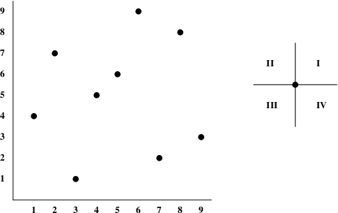
Let $\sigma=\sigma_{1}\ldots\sigma_{n}$ be a permutation in the symmetric group $S_{n}$ written in one-line notation. Then we will consider the graph of $\sigma$, $G(\sigma)$, to be the set of points $(i,\sigma_{i})$ for $i=1,\ldots,n$. For example, the graph of the permutation $\sigma=471569283$ is pictured in Figure 1. Then if we draw a coordinate system centered at a point $(i,\sigma_{i})$, we will be interested in the points that lie in the four quadrants I, II, III, and IV of that coordinate system as pictured in Figure 1. For any $a,b,c,d\in\mathbb{N}$ where $\mathbb{N}=\{0,1,2,\ldots\}$ is the set of natural numbers and any $\sigma=\sigma_{1}\ldots\sigma_{n}\in S_{n}$, we say that $\sigma_{i}$ matches the quadrant marked mesh pattern $MMP(a,b,c,d)$ in $\sigma$ if in $G(\sigma)$ relative to the coordinate system which has the point $(i,\sigma_{i})$ as its origin, there are $\geq a$ points in quadrant I, $\geq b$ points in quadrant II, $\geq c$ points in quadrant III, and $\geq d$ points in quadrant IV. For example, if $\sigma=471569283$, the point $\sigma_{4}=5$ matches the quadrant marked mesh pattern $MMP(2,1,2,1)$ since relative to the coordinate system with origin $(4,5)$, there are 3 points in $G(\sigma)$ in quadrant I, 1 point in $G(\sigma)$ in quadrant II, 2 points in $G(\sigma)$ in quadrant III, and 2 points in $G(\sigma)$ in quadrant IV. Note that if a coordinate in $MMP(a,b,c,d)$ is 0, then there is no condition imposed on the points in the corresponding quadrant. In addition, we shall consider patterns $MMP(a,b,c,d)$ where $a,b,c,d\in\mathbb{N}\cup\{\emptyset\}$. Here when one of the parameters $a$, $b$, $c$, or $d$ in $MMP(a,b,c,d)$ is the empty set, then for $\sigma_{i}$ to match $MMP(a,b,c,d)$ in $\sigma=\sigma_{1}\ldots\sigma_{n}\in S_{n}$, it must be the case that there are no points in $G(\sigma)$ relative to coordinate system with origin $(i,\sigma_{i})$ in the corresponding quadrant. For example, if $\sigma=471569283$, the point $\sigma_{3}=1$ matches the marked mesh pattern $MMP(4,2,\emptyset,\emptyset)$ since relative to the coordinate system with origin $(3,1)$, there are 6 points in $G(\sigma)$ in quadrant I, 2 points in $G(\sigma)$ in quadrant II, no points in $G(\sigma)$ in quadrant III, and no points in $G(\sigma)$ in quadrant IV. We let $\mathrm{mmp}^{(a,b,c,d)}(\sigma)$ denote the number of $i$ such that $\sigma_{i}$ matches the marked mesh pattern $MMP(a,b,c,d)$ in $\sigma$.

Note how the (two-dimensional) notation of Úlfarsson [13] for marked mesh patterns corresponds to our (one-line) notation for quadrant marked mesh patterns. For example,

Kitaev and Remmel [7] studied the distribution of quadrant marked mesh patterns in the symmetric group $S_{n}$ and Kitaev, Remmel, and Tiefenbruck [9, 10] studied the distribution of quadrant marked mesh patterns in $132$-avoiding permutations in $S_{n}$. In [8], Kitaev and Remmel studied the distribution of the statistics $\mathrm{mmp}^{(1,0,0,0)}$, $\mathrm{mmp}^{(0,1,0,0)}$, $\mathrm{mmp}^{(0,0,1,0)}$, and $\mathrm{mmp}^{(0,0,0,1)}$ in the set of up-down and down-up permutations. The main goal of this paper is to study the distribution of the statistics $\mathrm{mmp}^{(1,0,\emptyset,0)}$, $\mathrm{mmp}^{(0,1,0,\emptyset)}$, $\mathrm{mmp}^{(0,\emptyset,0,1)}$, and $\mathrm{mmp}^{(\emptyset,0,1,0)}$ in the set of up-down and down-up permutations. Given a permutation $\sigma=\sigma_{1}\ldots\sigma_{n}\in S_{n}$, we let $Des(\sigma)=\{i:\sigma_{i}>\sigma_{i+1}\}$. Then we say that $\sigma$ is an up-down permutation if $Des(\sigma)$ is the set of all even numbers less than or equal to $n$ and a down-up permutation if $Des(\sigma)$ is the set of all odd numbers less than or equal to $n$. That is, $\sigma$ is an up-down permutation if

and $\sigma$ is an down-up permutation if

Let $UD_{n}$ denote the set of all up-down permutations in $S_{n}$ and $DU_{n}$ denote the set of all down-up permutations in $S_{n}$. Given a permutation $\sigma=\sigma_{1}\ldots\sigma_{n}\in S_{n}$, we define the reverse of $\sigma$, $\sigma^{r}$, to be $\sigma_{n}\sigma_{n-1}\ldots\sigma_{2}\sigma_{1}$ and the complement of $\sigma$, $\sigma^{c}$, to be $(n+1-\sigma_{1})\ldots(n+1-\sigma_{n})$.

For $n\geq 1$, we let

We then have the following simple proposition.

In [8], we studied the distribution of the statistics $\mathrm{mmp}^{(1,0,0,0)}$, $\mathrm{mmp}^{(0,1,0,0)}$, $\mathrm{mmp}^{(0,0,1,0)}$, and $\mathrm{mmp}^{(0,0,0,1)}$ in the set of up-down and down-up permutations. It follows from Proposition 1 that the study the distribution of the statistics $\mathrm{mmp}^{(1,0,0,0)}$, $\mathrm{mmp}^{(0,1,0,0)}$, $\mathrm{mmp}^{(0,0,1,0)}$, and $\mathrm{mmp}^{(0,0,0,1)}$ in the set of up-down and down-up permutations can be reduced to the study of the following generating functions:

In the case when $x=1$, these generating functions are well known. That is, for any $(a,b,c,d)$, let $A_{2n}(1)=A^{(a,b,c,d)}_{2n}(1)$, $B_{2n+1}(1)=B^{(a,b,c,d)}_{2n+1}(1)$, $C_{2n}(1)=C^{(a,b,c,d)}_{2n}(1)$, and $D_{2n}(1)=D^{(a,b,c,d)}_{2n}(1)$. The operation of complementation shows that $A_{2n}(1)=C_{2n}(1)$ and $B_{2n_{1}}(1)=D_{2n-1}(1)$ for all $n\geq 1$. André [1, 2] proved that

and

In [8], we proved the following which can be viewed as a refinement of André’s results.

In this paper, we prove a different refinement of Adré’s results by studying the distribution of the statistics $\mathrm{mmp}^{(1,0,\emptyset,0)}$, $\mathrm{mmp}^{(\emptyset,0,1,0)}$, $\mathrm{mmp}^{(0,1,0,\emptyset)}$, and $\mathrm{mmp}^{(0,\emptyset,0,1)}$ in the set of up-down and down-up permutations. It follows from Proposition 1 that the study the distribution of the statistics $\mathrm{mmp}^{(1,0,\emptyset,0)}$, $\mathrm{mmp}^{(\emptyset,0,1,0)}$, $\mathrm{mmp}^{(0,1,0,\emptyset)}$, and $\mathrm{mmp}^{(0,\emptyset,0,1)}$ in the set of up-down and down-up permutations can be reduced to the study of the following generating functions:

The main goal of this paper is prove the following theorem.

Here ${}_{2}F_{1}(a,b;c;z)=\sum_{n=0}^{\infty}\frac{(a)_{n}(b)_{n}}{(c)_{n}}\frac{z^{n}}{n!}$ where $(x)_{n}=x(x-1)\cdots(x-n+1)$ if $n\geq 1$ and $(x)_{0}=1$.

One can use these generating functions to find some initial values of the polynomials $A^{(1,0,\emptyset,0)}_{2n}(x)$, $B^{(1,0,\emptyset,0)}_{2n-1}(x)$, $C^{(1,0,\emptyset,0)}_{2n}(x)$, and $D^{(1,0,\emptyset,0)}_{2n-1}(x)$. For example, we have used Mathematica to compute the following tables.

$n$ $A^{(1,0,\emptyset,0)}_{2n}(x)$ 0 1 1 x 2 $x(2+3x)$ 3 $x\left(16+30x+15x^{2}\right)$ 4 $x\left(272+588x+420x^{2}+105x^{3}\right)$ 5 $x\left(7936+18960x+16380x^{2}+6300x^{3}+945x^{4}\right)$ 6 $x\left(353792+911328x+893640x^{2}+429660x^{3}+103950x^{4}+10395x^{5}\right)$


$n$ $B^{(1,0,\emptyset,0)}_{2n+1}(x)$ 0 1 1 $2x$ 2 $x\left(7+9x\right)$ 3 $x\left(77+135x+60x^{2}\right)$ 4 $x\left(1657+3444x+2310x^{2}+525x^{3}\right)$ 5 $x\left(58457+135945x+112770x^{2}+40950x^{3}+5670x^{4}\right)$ 6 $x\left(3056557+7715664x+7347945x^{2}+3395700x^{3}+777625x^{4}+72765x^{5}\right)$


$n$ $C^{(1,0,\emptyset,0)}_{2n}(x)$ 0 1 1 1 2 $x\left(2+3x\right)$ 3 $x\left(7+35x+19x^{2}\right)$ 4 $x\left(77+581x+571x^{2}+156x^{3}\right)$ 5 $x\left(1657+16428x+21066x^{2}+9738x^{3}+1587x^{4}\right)$ 6 $x\left(58457+712579x+1079747x^{2}+652452x^{3}+180240x^{4}+19290x^{5}\right)$


$n$ $D^{(1,0,\emptyset,0)}_{2n+1}(x)$ 0 1 1 $x(1+x)$ 2 $x\left(2+9x+5x^{2}\right)$ 3 $x\left(16+110x+113x^{2}+33x^{3}\right)$ 4 $x\left(272+2492x+3288x^{2}+1605x^{3}+279x^{4}\right)$ 5 $x\left(7936+90384x+139756x^{2}+87456x^{3}+25365x^{4}+2895x^{5}\right)$ 6 $x\left(353792+4803040x+8323816x^{2}+6110100x^{3}+2297778x^{4}+444045x^{5}+35685x^{6}\right)$

The outline of this paper is as follows. In section 2, we shall prove theorem 2. Then in section 3, we shall show how several of the entries of the tables above can be explained. In particular, we will derive formulas for the coefficient of the highest and lowest coefficient of $x$ in the polynomials the polynomials $A^{(1,0,\emptyset,0)}_{2n}(x)$, $B^{(1,0,\emptyset,0)}_{2n+1}(x)$, $C^{(1,0,\emptyset,0)}_{2n}(x)$, and $D^{(1,0,\emptyset,0)}_{2n+1}(x)$ as well as formulas for the second highest and second lowest coefficient of $x$ in these polynomials. Finally, in section 3, we shall discuss some connections with our previous work [8] on quadrant marked mesh patterns in alternating permutations as well as some directions for further research.

The proof of all parts of Theorem 2 proceed in the same manner. That is, there are simple recursions satisfied by the polynomials $A^{(1,0,\emptyset,0)}_{2n}(x)$, $B^{(1,0,\emptyset,0)}_{2n+1}(x)$, $C^{(1,0,\emptyset,0)}_{2n}(x)$, and $D^{(1,0,\emptyset,0)}_{2n+1}(x)$ based on the possible positions of 1 in an up-down or a down-up permutation.

References

- [1] D. André, Développements de sec x et de tang x, C. R. Acad. Sci. Paris, 88 (1879), 965–967.
- [2] D. André, Mémoire sur les permutations alternées, J. Math. Pur. Appl., 7 (1881), 167–184.
- [3] S. Avgustinovich, S. Kitaev and A. Valyuzhenich, Avoidance of boxed mesh patterns on permutations, preprint.
- [4] P. Brändén and A. Claesson, Mesh patterns and the expansion of permutation statistics as sums of permutation patterns, Elect. J. Comb. 18(2) (2011), #P5, 14pp.
- [5] Í. Hilmarsson, I. Jónsdóttir, S. Sigurdardottir, H. Úlfarsson and S. Vidarsdóttir, Partial Wilf-classification of small mesh patterns, in preparation.
- [6] S. Kitaev, Patterns in permutations and words, Springer-Verlag, (2011).
- [7] S. Kitaev and J. Remmel, Quadrant marked mesh patterns, J. Integer Sequences, 12 Issue 4 (2012), Article 12.4.7.
- [8] S. Kitaev and J. Remmel, Quadrant marked mesh patterns in alternating permutations, preprint.
- [9] S. Kitaev, J. Remmel and M. Tiefenbruck, Quadrant marked mesh patterns in 132-avoiding permutations I, preprint.
- [10] S. Kitaev, J. Remmel and M. Tiefenbruck, Quadrant marked mesh patterns in 132-avoiding permutations II, in preparation.
- [11] N. J. A. Sloane, The on-line encyclopedia of integer sequences, published electronically at http://www.research.att.com/˜njas/sequences/.
- [12] R.P. Stanley, Enumerative Combinatorics, vol. 2, Cambridge University Press, (1999).
- [13] H. Úlfarsson, A unification of permutation patterns related to Schubert varieties, arXiv:1002.4361 (2011).