Nonparametric Edge Detection in Speckled Imagery
Abstract
We address the issue of edge detection in Synthetic Aperture Radar imagery. In particular, we propose nonparametric methods for edge detection, and numerically compare them to an alternative method that has been recently proposed in the literature. Our results show that some of the proposed methods display superior results and are computationally simpler than the existing method. An application to real (not simulated) data is presented and discussed.
Keywords:
Edge detection, hypothesis testing, image analysis, multiplicative noise, small samples, speckle , SAR1 Introduction
Synthetic Aperture Radar (SAR) images are an important source information in many applications, such as urban planning, environmental monitoring, crop management, oil prospection, mining exploration, wind detection, animal life detection, among others. A SAR is a coherent radar of high resolution that works on-board using a synthetic antenna of a movable platform, like an airplane or a satellite, covering extended surfaces and producing images. SAR systems employ the Doppler effect and processes the signal obtaining high spatial resolution in the direction of the platform motion [24].
During the data collection, the target remains illuminated under the antenna beam for a few moments and is observed by the radar from positions induced by its movement throughout the platform trajectory. The radar illuminates the target with a succession of pulses of a given frequency. The energy is propagated in all directions, and part of it returns to the antenna (this return is called ‘echo’). The sensor measures both the intensity and the delay between the signals sent from and received back by the antenna. The image is then formed based on the energy returned by each point on the surface.
Some of the most important features of the SAR sensor for remote sensing are:
- 1.
The active nature of the instrument makes it independent of other illumination sources, being able to gather images at any time.
- 2.
Microwaves intensity are not significantly affected by the presence of clouds, so image acquisition is possible in most metheorological conditions and in regions with permanent cloud coverage.
- 3.
SAR images can have high spatial resolution, e.g. of less than one meter, thus making the study of small scale phenomena possible.
- 4.
SAR images contain complementary information to that provided by optical images. The selection of frequency band, polarization and angle of incidence in SAR imagery allows the discrimination of different surface properties.
A SAR sensor emits and receives electromagnetic waves of complex nature and, therefore, the received signal can be stored in different formats: complex, intensity, amplitude and phase [22].
In a SAR image, it is possible to distinguish several types of roughness or texture, according to which one can classify the different types of covers:
- 1.
Homogenous areas: Surfaces of very little texture; for example, crops, deforestation, and, under some conditions, snow, water or ice.
- 2.
Heterogeneous areas: Surfaces that display some texture; for example, forests on not very pronounced reliefs, among others.
- 3.
Extremely heterogeneous areas: Surfaces with intense texture; for instance, urban areas, among others.
“Texture”, in the context of SAR imagery, should be understood as a measure of the number of objects in a cell of the size the of the wavelength employed by the sensor. A fine texture corresponds to a large number of objects per cell, while coarse or extremely heterogeneous textures are those for which only a few objects are counted per cell. The Japanese Earth Resources Satellite JERS-1, for instance, operates on L-Band ( GHz, cm wavelength) and the European Remote Sensing Satellites ERS-1 and ERS-2 use C-Band ( GHz, cm wavelength).
A problem of paramount importance in the analysis of images is segmentation: the process that divides an image in its constituent parts or objects. Its main goal is to group image areas that have similar characteristics. One of the basic principles in the segmentation process is the detection of discontinuities. Edges are the borders of the objects and are therefore quite useful for their segmentation, registration and identification. Edges can be thought as the locations where abrupt changes in intensity or in other important characteristic occur.
The quality of SAR images is degraded by speckle, a degradation which follows from the use of coherent illumination, i.e., when the signal phase is employed in the image formation. Such degradation is characteristic of technologies that employ microwaves, sonar, laser and ultrasound.
The presence of speckle makes edge detection difficult, since most algorithms identify regions using local characteristics. Though speckle should not be regarded as noise, since it has a deterministic nature and is reproducible, from the image practitioner viewpoint it can be considered a random effect and can be conveniently described by stochastic laws; c.f. Richards [24, Sec. 4.3.1]. It is not convenient to only use pointwise information when detecting edges under speckle; it is necessary to analyze the image using sets of pixels that provide local information [15].
Different approaches can be used to locate the edges between regions in a SAR image. A particularly attractive and well performing statistical method was proposed by Gambini et al. [14]. It is based on the family of distributions, which can be successfuly used to describe areas with different degrees of homogeneity [11, 13, 18, 19].
In this work we consider intensity imagery, described by the law. This distribution is indexed by the number of looks , the scale parameter and the roughness parameter . The former can be controlled when generating the image or in postprocessing stages, and is a measure of the signal-to-noise ratio [24, Sec. 4.3.1]. The value of the roughness parameter is of interest in many applications, since it can be used as an indicator of land type. The scale parameter relates to the relative power between the reflected and incident signals [13].
Figure 1 presents three different targets and the corresponding values (or range of values) of the roughness parameter (). Small values of (e.g., ) are associated with homogeneous areas, such as pastures. Values of are characteristic of heterogeneous regions, for example forests. Finally, larger values of (say, ) are observed in extremely heterogeneous areas, such as urban regions [6, 19].

Our chielf goal is to develop and assess new methods for edge detection in SAR images using computationally efficient nonparametric statistical inference. Gambini et al. [14] showed that a method based on maximum likelihood, which is presented in Section 3.1, is more precise than four commonly used techniques: two based on raw data (maximum discontinuity and fractal dimension) and two based on estimates (maximum discontinuity and anisotropic smoothed roughness). Our numerical evaluation reveals that some of the edge detection strategies we propose in this paper outperform the best method available to date, i.e., maximum likelihood [14], at considerably lower computational cost.
The paper unfolds as follows. Section 2 presents the model. Section 3 discusses the use of nonparametric statistics for SAR image detection, while Section 4 presents the results. An application that uses real (not simulated) data is presented and discussed in Section 5. Conclusions and directions for future work are outlined in Section 6.
2 The multiplicative model
The physics of SAR image formation leads to the multiplicative model: the random field describing the observations can be viewed as the product of two independent random fields, which are not observed directly, namely: and . The former () models the properties of the imaged area (backscatter), whereas the latter () models the speckle noise due to the use of coherent illumination.
Speckle noise in intensity -looks format follows a Gamma distribution, denoted by , whose density is given by
In SAR images modeling, the smallest value of is , which corresponds data with the highest spatial resolution, at the expense of lower signal-to-noise ratio. The number can be assumed to be known or estimated beforehand from the entire image. We shall assume that the number of looks is known.
The backscatter exhibits different degrees of homogeneity, and different models have been used to encompass this characteristic. The reciprocal of Gamma distribution is a useful and tractable model [1, 6, 8, 12, 13, 14, 15, 18, 19, 20, 21, 26]. The random variable follows this law, denoted , if its density function is
Let and be two independent random variables. It can be shown that the random variable follows a distribution, denoted , whose density is
| (1) |
where is the roughness parameter, is the scale parameter and is the number of looks [13].
In this work we consider independent samples. Correlated fields are treated by Bustos et al. [5].
The -th noncentral moment of is given by
| (2) |
if , and otherwise.
The distribution is very attractive for modeling data with speckle noise, due to its mathematical tractability and because it is able to describe information from most types of areas.
Figure 2 shows densities, where is the value of that delivers unit expected value for given and . The densities are presented in semilogarithmic scale, showing that they have heavy (linear) tails with respect to the Gaussian distribution which displays quadratic behavior. It is noticeable that larger values of lead to larger variances; in fact, the variance is not finite when .

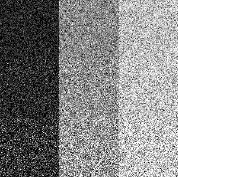
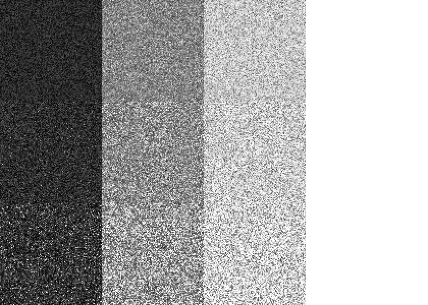
Figure 3 shows nine patches of speckled data for one, three and eight looks. Each patch consists of images with varying roughness and contrast: each column shows images with same mean (, and , left to right) while rows from bottom to top show images with . It can be readily seen that finding edges in speckled data can be a hard task due to the existing local variation.

Gambini et al. [14], Gambini et al. [15] used an analogy estimator based on moments of order and . Since we wish to extend their work, we shall use the same approach.
Let be a vector of independent identically distributed random variables, with common distribution , , and known. Define the -th sample moment as
with and (that is the reason why we assume rather than ).
Replacing the population moments by their sample counterparts, and the parameters by the corresponding estimators, we arrive at the following system of two equations:
| (3) |
and
which leads to the following equation that can be solved numerically in order to obtain an estimator for :
By plugging the value of into equation (3) we obtain .
Frery et al. [12] showed that computing ML estimators for the family is prone to severe numerical instabilities, and they proposed an iterative algorithm that alleviates this problem. Recently Pianto and Cribari-Neto [23] analyzed this issue and found that it is related to a flattening of the likelihood function, and they proposed a correction based on resampling. Cribari-Neto et al. [8] showed that ML estimators for that distribution can be quite biased, and they evaluated the effectiveness of improving them by several resampling techniques. Vasconcellos et al. [26] proposed an analytical bias correction for ML estimators; they showed that there is a wide range of practical situations for which the corrected estimator effectively reduces both bias and mean square error of the original ML estimator. Bustos et al. [6] derived M-estimators and showed that such robust estimators are superior to the classical estimators in the presence of corner reflectors, a common source of contamination in SAR images. Allende et al. [1] derived AM-estimators (M estimators with asymmetric influence functions), motivated by the shape of the density. Overall, their estimators outperform both ML and M-estimators.
In the next section we shall summarize the main techniques that are available for edge detection in SAR imagery, with special emphasis on those that explicitly employ statistical models and techniques.
3 Edge detection in SAR imagery
Statistical edge detection is described in Bovik et al. [3]. These authors introduced nonparametric statistics for edge detection under Gaussian additive noise. They showed the usefulness of the median and the Wilcoxon-Mann-Whitney tests for edge detection with the help of a sample image interpreted visually.
Fesharaki and Hellestrand [10] proposed an algorithm for edge detection by using a -test, while Beauchemin et al. [2] used a nonparametric alternative based on the Wilcoxon-Mann-Whitney statistics for detecting changes between adjacent pixel neighborhoods. Although these tests may be appropriate for specific types of images, they may not detect changes in local grey level values in images with low signal-to-noise ratios, as is the case of SAR imagery.
Hoon Lim and Ju Jang [16] compared two-sample tests for edge detection in noisy images. Later Lim [17] described a new edge detector based on the robust rank-order test, an alternative to the Wilcoxon test, using windows for detecting all possible edges in noisy images. This method is based on testing whether an window is partitioned into two sub-regions.
The detection of edges in images with speckle noise has been studied by many authors, and a variety of techniques are presented and compared by Gambini et al. [14], Gambini et al. [15], whose proposed approach outperforms all competing procedures with an acceptable computational cost. Their method is based on fitting contours of objects and regions using B-splines; such curves depend on a few parameters and can be easily computed from control points and smoothness conditions [4].
Gambini et al. [14], Gambini et al. [15] used amplitude data for finding edges between different regions. Such data, if squared, follow the distribution. Under this model, the regions of the image with different degrees of homogeneity are characterized by the parameters of the distribution. If a point belongs to the edge of the object, then a sudden change in the parameter values is expected in its neighborhood.
In what follows we present five techniques for detecting edges in SAR images, namely the method proposed by Gambini et al. [14], Gambini et al. [15], and four alternative techniques based on ranks. The two main advantages of nonparametric tests are that
- 1.
they do not depend upon the data distribution, and
- 2.
they are robust to extreme observations.
These features are of particular interest in the case at hand, namely, speckled imagery.
3.1 The Gambini algorithm for edge detection
This is an iterative procedure that refines an initial region until the final result is achieved. It is based on the fact that if a point belongs to the object edge, then a sample taken from its neighbourhood should exhibit a change in the parameter values and, therefore, should be considered a transition point.
Consider image segments, , of the form , where is the centroid of the initial region, the extreme is a point outside the region and is the angle between two successive segments, as shown in Figure 4.

Consider a strip of pixels around each segment , as illustrated in Figure 5, partitioned into two areas by a candidate edge point (the small red dot). The observations within the strip are taken to come from two different models, namely one corresponding to the object (the dark area in Figure 5) and the other from the background .

The parameters and index the region and its background, respectively, and their estimation is described in Section 2; note that the estimators depend upon the the transition point .
In order to find the transition point on each segment , an objective function is considered: the sample likelihood, which is given by
where is the number of observations in the strip around segment lying between and , and is the number of observations in the strip lying between and .
In order to find the transition point, we maximize the log-likelihood function
for every possible value of . Using equation (1), and assuming that is known,
| (4) |
Finally, the estimated transition point on the segment is given by
| (5) |
Figure 6 shows typical values of the objective function, taken along a straight line segment.

3.2 Nonparametric edge detection
In the typical two-sample situation, the experimenter has two samples from possibly different populations, and wishes to use a statistical test to determine whether the null hypothesis that the two populations are identical should be rejected. That is, the experimenter wishes to identify differences between the two populations on the basis of their random samples.
An intuitive approach to the two-sample problem is to combine both samples into a single ordered sample, and assign ranks to the observations, regardless the source population. A possible test statistic is the sum of the ranks assigned to each population. If such a sum is small (large), there is indication that the values from that population tend to be smaller (larger) than the values obtained from the other population. The null hypothesis should be rejected if the sum of the ranks associated with one sample is considerably larger than the other sum.
3.2.1 The Mann-Whitney test
The data consist of samples from two populations. Let denote the random variables sampled from population and denote the variates obtained from population . Assign the ranks to the individual observations in the combined sample. Let and denote the ranks assigned to and for all and . If two or more sample values are equal (ties), assign to each the average of the ranks that would have been assigned had there been no ties.
The following assumptions are made:
- 1.
Both samples are random samples from the respective populations.
- 2.
In addition to independence within each sample, there is mutual independence between the two samples.
- 3.
The measurement scale is at least ordinal.
Let and be the distribution functions of and , respectively. We wish to test
In many situations, as in edge detection, differences between distributions imply that does not equal . Therefore, we can rewrite the above hypotheses as
The null hypothesis can be tested using the Mann-Whitney test, which is unbiased and consistent. The test statistic is computed as follows. When there are no or just a few ties, the sum of the ranks assigned to the sample from population can be used as a test statistic:
When the number of ties is large, one can subtract the (null) mean from and divide the resulting difference by the (null) standard deviation to get
3.2.2 The Kruskal-Wallis test
The Mann-Whitney test for two independent samples was extended to the problem of analyzing independent samples, , by Kruskal and Wallis in 1952. The experimental situation is that random samples have been obtained from possibly different populations, and one wishes to test the null hypothesis that all populations are identical. The Kruskal-Wallis test statistic is a function of the ranks of the observations in the combined sample (like the Mann-Whitney test statistic).
The data consist of random samples of possibly different sizes. Denote the th random sample of size by . Then, the data may be arranged in columns:
| Sample | Sample | Sample | |
|---|---|---|---|
Let denote the total number of observations, i.e., . Assign rank to the smallest of the observations, rank to the second smallest observation, and so on. Let be the sum of the ranks assigned to the th sample:
| (6) |
Compute for each sample. Under ties, assign the average rank to each tied observation, as in the previous test.
The following assumptions are made:
- 1.
All samples are random samples from their respective populations.
- 2.
In addition to independence within each sample, there is mutual independence amongst samples.
- 3.
The measurement scale is at least ordinal.
- 4.
Either the population distribution functions are identical or else some of the populations tend to yield larger values than the remaining populations.
The null and alternative hypotheses are
| at least one of the remaining populations. |
Since the Kruskal-Wallis test is designed to be sensitive against differences among means in the populations, the alternative hypothesis is sometimes stated as
The populations do not all have identical means.
The test statistic is defined as
| (7) |
where
3.2.3 The squared ranks test for variances
The squared ranks test can be used to assess equality of variances across two or more independent, random samples which have been measured using a scale that is at least interval [7].
The data consist of the two random samples. Let denote a random sample of size from population and represent a random sample of the size from population . Define
and
where and are the two sample means.
Assign ranks to to the combined sample, as usual. If several values of and/or are equal (ties), assign to each the average of the ranks that would have been assigned to them had there been no ties.
The required assumptions can be stated as follows:
- 1.
Both samples are random samples from the respective populations.
- 2.
In addition to independence within each samples, there is mutual independence between samples.
- 3.
The measurement scale is at least interval.
The null and alternative hypotheses are
If there are no values of tied with values of , the sum of the squared ranks assigned to population can be used as a test statistic:
If there are ties, subtract the (null) mean from and divide the difference by the (null) standard deviation to get
where , and is the average of the squared ranks of both samples combined:
also,
3.2.4 The TPE empirical statistic
The empirical statistic TPE is also based on ranges, and is well suited for situations where one wishes to test whether two samples come from the same distribution or from distributions with different means and/or variances. The data consist of the two random samples. Let denote a random sample of size from population and let denote a random sample of the size from population . Assign ranks , and compute , , and . The mean rank of the combined sample is . The empirical statistic TPE is .
3.3 Proposal
Our chief goal is to perform edge detection in SAR images using the aforementioned nonparametric tests statistics instead of the likelihood function presented in equation (4).
The new noparametric edge estimates on segment are given by
- 1.
Mann-Whitney estimate: ,
- 2.
Kruskal-Wallis estimate: ,
- 3.
Squared Ranks estimate: , and
- 4.
TPE empirical estimate: ,
where denotes the edge candidate coordinate.
Figure 7 shows values of the of the Mann-Whitney, Kruskal-Wallis, Squared Ranks and the TPE Empirical test statistics taken along a straight line segment of simulated data. The corresponding positions of the maxima (Mann-Whitney, Kruskal, Variance) or minimum (TPE) are taken to be the transition point between the two regions. Data generation was carried in such a way that the true transition point is at . We note that all four methods successfuly identify the edge point.


4 Numerical results
This section presents simulations performed to obtain a quantitative assessment of the performances of the proposed edge detection methods. All simulations were run on personal computers with Intel© Pentium© IV CPUs of GHz running Windows XP operating system. The programming language used was Ox version [9, for details, see]. All graphics were produced using R version 2.6.1 [27].
We shall evaluate the errors made when estimating the edge point (local error) in several parametric situations. For each situation, simulated rectangular windows of sizes ( rows, columns) are filled with with samples from distributions.
Each window is composed of two halves, and we consider all possible combinations of roughness parameters and , and number of looks . Here, () denotes the value of used for data generation to the left (right) of the true edge point. These values span a variety of images often encountered in practice, ranging from single-loook to smoothed multi-look. The scale parameter equals
so that the distribution mean equals one in all situations.
It is noteworthy that edge detection algorithms are therefore evaluated in a very difficult situation, namely, when the areas have the same mean and only differ in texture.
Situations in which are not considered, since they entail no edge. We thus consider (, and ) cases. For each of them, we simulate windows. In each of these windows, the edge is detected by the five techniques already described, and the error is defined as the absolute difference between the true edge (which is located at position 50) and the detected edge.
The errors are stored in an -dimensional array defined in the following way:
where , , is the transition point identified by method in the th sample. Note that ranges in the set
Let denote the percentage of times in which the estimated edge is more than pixels apart from the true value, using method , i.e.,
These are the error rates we report. Method is considered to be more accurate than method whenever , i.e., whenever the percentage of errors of method is smaller than that of method , except for errors up to 5 pixels.
Figure 8 depicts four of the situations assessed: three where single () look data are contrasted (Figures 8(a), 8(b) and 8(c)), and one with looks (Figure 8(d)). The single look data show the differences between heterogeneous (, Figure 8(a)), and homogeneous (, Figure 8(b)); , Figure 8(c)) areas and strips of varying roughness. The data only presents the difference between a homogenous area () and several other strips (Figure 8(d)). The areas to the left are formed by independent draws from the distribution. The strips to the right are formed by independent outcomes of the law with . The contrast among regions has been enhanced in order to make visualization easier; actual data are harder to differentiate.


Figure 9 summarizes the main results of our study, regarding error rates. Each column presents the error rates as a function of , the number of looks, provided a roughness for the left half of the strip . We notice that the error rates are consistent with respect to , since their behavior does not alter significantly. Different lines, for a given , show the behavior of the error rates as a function of the roughness. Mann-Whitney is the only nonparametric technique that exhibits poor performance, but only when ; all other procedures are competitive. Kruskal edge detection behaves similarly to Gambini procedure, with minor differences that do not consistently benefit either. TPE and Variance are slightly worse than Kruskal and Gambini, mainly when multilook () imagery is used. The error rates are consistently larger when the left and right roughnesses are similar; notice that the curves peaks shift to the left from top to bottom. Overall, the Kruskal and Gambini error rates decrease as the number of looks increases, the same pattern holding for the degree of heterogeneity.


Figure 10 presents the average execution times for the and situation, which is representative of all remaining execution times. As Figure 10(a) shows, the time spent by Gambini decreases as the value of increases, but it is consistently larger than the nonparametric techniques detection times. The differences in execution times are of three orders of magnitude and occur in all of the situations herein assessed. Figure 10(b) shows the average execution times of the nonparametric methods, which never exceeded one second; Kruskal was the fastest followed by Mann-Whitney.


As noted earlier, the hardest task one can face is the discrimination of regions indexed by similar parameter values. Table 1 presents a subset of our numerical results and focuses on the most challenging cases. It is clear from the figures in this table that Kruskal is consistently faster than Gambini, reaching a scale of in some cases. The error rates of the two methods are similar.
| Gambini | Kruskal | |||||
|---|---|---|---|---|---|---|
| Situation | Error | Time | Error | Time | ||
5 Application to real data
Figure 11 presents a SAR image for which the estimated number of looks is . The window considered has pixels, and was obtained over agricultural fields of Oberpfaffenhofen, Germany, in the L-band, by the ESAR sensor [25].
The original data displayed almost no differences, and it was enhanced for visual purposes. Two main regions can be observed, namely: the dark (left) and light (right) areas. The estimated roughness parameter in both areas are approximately equal to 7.5 (i.e., ), thus implying that both areas are slightly heterogeneous, probably due to relief.
An edge was detected in each of five non-overlapping strips of pixels. The Mann-Whitney, Kruskal-Wallis and Gambini estimates agree and are indicated by red dots in the middle of each strip. The estimates, thus, provide accurate starting points for any subsequent edge detection algorithm.

6 Conclusions
Our chief goal was to propose alternative techniques for edge detection in speckled imagery. The proposed methods were compared to that of Gambini et al. [14], Gambini et al. [15]. The techniques here assessed do not try to eliminate existing speckle, but to extract information from its statistical properties. The model used to describe these data is the distribution, which Mejail et al. [18], Mejail et al. [19] show can be used as an universal model.
The methods under assessment aim at identifying edges between regions with different degrees of roughness, which, in turn, is determined by , the roughness parameter of the distribution. Homogenous, e.g., pastures, heterogeneous regions, e.g., forest, and very heterogeneous regions, e.g., urban, targets are considered.
In order to compare the performances of the five methods, a Monte Carlo experiment was carried out. Two criteria were employed in the comparison, namely: the error made in detecting an edge and the execution time. The thoughest setting was considered, namely, when the areas on both sides of the edge have the same mean and number of looks, differing only on the roughness.
From the experimental results it was observed that the Kruskal detector performed slightly better than Gambini. Compared with the TPE, Variance and Mann-Whitney detectors, the Kruskal performed much better.
It is noteworthy that all detection methods perform well when the edge separates areas with very different degress of roughness.
When the generated image represents homogenous zones, the error frequencies of all methods are relatively high, nevertheless this problem is alleviated by increasing the number of looks , causing the edge detection to become more accurate.
The Kruskal detector displays the best results, both with respect to error and execution time. The latter is, in many cases, times smaller than that of Gambini.
The TPE method for edge detection performs well when differs from by at least three units.
Mann-Whitney has good performance (both in terms of error rate and speed) when . When the method is unable to locate the edge, mostly because it only accounts for the ranks of one of the samples.
Overall, our results suggest that the Gambini edge detection technique can be successfully replaced by our Kruskal. By doing so, one achieves similar precision at a much lower computational cost (the latter is approximately one thousand times faster).
A promising line of research is the use of stochastic distances, as derived by Nascimento et al. [21].
Acknowledgements
The authors gratefully acknowledge research grants from Capes and CNPq. We also thank an anonymous referee for comments and suggestions.
References
- [1] H. Allende, A.C. Frery, J. Galbiati, L. Pizarro, M-estimators with asymmetric influence functions: the distribution case, Journal of Statistical Computation and Simulation 76 (2006) 941–956.
- [2] M. Beauchemin, K.P.B. Thomson, G. Edwards, On nonparametric edge detection in multilook SAR images, IEEE Transactions on Geoscience and Remote Sensing 36 (1998) 1826–1829.
- [3] A.C. Bovik, T.S. Huang, D.C. Munson, Nonparametric-tests for edge-detection in noise, Pattern Recognition 19 (1986) 209–219.
- [4] P. Brigger, J. Hoeg, M. Unser, B-spline snakes: A flexible tool for parametric contour detection, IEEE Transactions on Image Processing 9 (2000) 1484–1496.
- [5] O.H. Bustos, A.G. Flesia, A.C. Frery, M.M. Lucini, Simulation of spatially correlated clutter fields, Communications in Statistics – Simulation and Computation 38 (2009) 2134–2151.
- [6] O.H. Bustos, M.M. Lucini, A.C. Frery, M-estimators of roughness and scale for modelled SAR imagery, Eurasip Journal on Applied Signal Processing 2002 (2002) 105–114.
- [7] W.J. Conover, Practical nonparametric statistics, John Wiley & Sons, Inc, 1980.
- [8] F. Cribari-Neto, A.C. Frery, M.F. Silva, Improved estimation of clutter properties in speckled imagery, Computational Statistics & Data Analysis 40 (2002) 801–824.
- [9] J.A. Doornik, Object-Oriented Matrix Programming Using Ox, Timberlake Consultants Press & Oxford, London, 3 edition, 2002.
- [10] M.N. Fesharaki, G.R. Hellestrand, A new edge detection algorithm based on a statistical approach, in: International Symposium on Speech, Image Processing and Neural Networks (ISSIPNN), volume 1, pp. 21–24.
- [11] C.C. Freitas, A.C. Frery, A.H. Correia, The polarimetric G distribution for SAR data analysis, Environmetrics 16 (2005) 13–31.
- [12] A.C. Frery, F. Cribari-Neto, M.O. de Souza, Analysis of minute features in speckled imagery with maximum likelihood estimation, Eurasip Journal on Applied Signal Processing 2004 (2004) 2476–2491.
- [13] A.C. Frery, H.J. Müller, C.C. Freitas, S.J. Siqueira, A model for extremely heterogeneous clutter, IEEE Transactions on Geoscience and Remote Sensing 35 (1997) 648–659.
- [14] J. Gambini, M. Mejail, J. Jacobo-Berlles, A.C. Frery, Accuracy of edge detection methods with local information in speckled imagery, Statistics and Computing 18 (2008) 15–26.
- [15] J. Gambini, M.E. Mejail, J. Jacobo-Berlles, A.C. Frery, Feature extraction in speckled imagery using dynamic B-spline deformable contours under the model, International Journal of Remote Sensing 27 (2006) 5037–5059.
- [16] D. Hoon Lim, S. Ju Jang, Comparison of two-sample tests for edge detection in noisy images, Journal of the Royal Statistical Society: Series D (The Statistician) Volume 51 Issue 1 (2002) 21–30.
- [17] D.H. Lim, Robust edge detection in noisy images, Computational Statistics & Data Analysis 50 (2006) 803–812.
- [18] M.E. Mejail, A.C. Frery, J. Jacobo-Berlles, O. Bustos, Approximation of distributions for SAR images: Proposal, evaluation and practical consequences, Latin American Applied Research 31 (2001) 83–92.
- [19] M.E. Mejail, J.C. Jacobo-Berlles, A.C. Frery, O.H. Bustos, Classification of SAR images using a general and tractable multiplicative model, International Journal of Remote Sensing 24 (2003) 3565–3582.
- [20] E. Moschetti, M.G. Palacio, M. Picco, O.H. Bustos, A.C. Frery, On the use of Lee’s protocol for speckle-reducing techniques, Latin American Applied Research 36 (2006) 115–121.
- [21] A.D.C. Nascimento, R.J. Cintra, A.C. Frery, Hypothesis testing in speckled data with stochastic distances, IEEE Transactions on Geoscience and Remote Sensing 48 (2010) 373–385.
- [22] C. Oliver, S. Quegan, Understanding Synthetic Aperture Radar Images, Artech House, Boston., 1998.
- [23] D.M. Pianto, F. Cribari-Neto, Dealing with monotone likelihood in a model for speckled data, Computational Statistics and Data Analysis 55 (2011) 1394–1409.
- [24] J.A. Richards, Remote Sensing with Imaging Radar, Springer, 2009.
- [25] X. Su, C. He, Q. Feng, X. Deng, H. Sun, A supervised classification method based on conditional random fields with multiscale region connection calculus model for sar image, IEEE Geoscience and Remote Sensing Letters 8 (2011) 497–501.
- [26] K.L.P. Vasconcellos, A.C. Frery, L.B. Silva, Improving estimation in speckled imagery, Computational Statistics 20 (2005) 503–519.
- [27] W.N. Venables, B.D. Ripley, Modern Applied Statistics with S, Statistics and Computing, Springer, New York, 4 edition, 2002.