UV Cascade in Classical Yang-Mills Theory
Abstract:
We study the real-time behavior of classical Yang-Mills theory under initial conditions with nonperturbatively large, infrared field amplitudes. Our lattice study confirms the cascade of energy towards higher momenta and lower occupancy, which occurs via a scaling solution . Above a characteristic scale , falls exponentially; below , . We find no evidence for different infrared exponents or for infrared occupancies in excess of those described by this scaling solution. We also investigate what the fate of large occupancies would be, both in the electric and the magnetic sector.
Keywords:
Lattice, Classical Yang-Mills, gauge fixing, screening1 Introduction
Consider classical Yang-Mills theory. If the initial conditions contain field energy in some region of space with vacuum around, we know that after a while the energy will be in an expanding nearly-spherical shell of outward moving waves. But if the initial conditions are statistically spatially homogeneous, the fields will re-interact indefinitely. Now classical Yang-Mills theory, like all nonlinear classical field theories, has no equilibrium; there is infinite phase space in the deep ultraviolet. So the energy should cascade into the ultraviolet, spreading with ever smaller amplitude over ever more field modes. But exactly how does this cascade actually occur?
Recently there has been renewed interest in this question, because classical Yang-Mills theory should describe the behavior of weakly-coupled, quantum Yang-Mills theory when the mean occupancy is high, for the most important in a system. The initial conditions after a heavy ion collision, in the limit of large and high energy nuclei, are expected to involve high-occupancy, effectively classical fields [1]. It is not clear to us how realistic the classical field description is phenomenologically; also, the initial conditions for a heavy ion collision are spatially inhomogeneous and anisotropic. Nevertheless, we will consider the homogeneous and isotropic case as an interesting warmup problem and lesson in the behavior of classical Yang-Mills theory. At minimum we believe that it is interesting to study the behavior of classical Yang-Mills theory in its own right, especially to establish its differences from scalar field theory.
Quite recently two papers have considered essentially the problem we raise; Yang-Mills theory at weak coupling and with initial conditions with high enough typical occupancy that the behavior is that of classical fields (at least for some period of time). Two of us argued [2] that the cascade into the ultraviolet would proceed with the dominant momentum scale (the scale where most of the energy density resides) growing with time as . The occupancy at this scale would behave as , and the occupancy for would scale as . (The same scaling for was found for scalar field theory much earlier by Micha and Tkachev [3].) On the same day, a paper by Blaizot, Gelis, Liao, McLerran and Venugopalan [4] came to similar conclusions, except that they argued that there could in addition be the formation of a condensate of infrared excitations, carrying most of the particle number, but a minority of the energy density, in the system. A recent numerical study of the problem by Berges, Sexty and Schlichting [5] did not try to determine the scaling of momentum or occupancy with time, but investigated the infrared tail of the spectrum. Contrary to the arguments of [2, 4], they found , with at early times and transforming to at late times (an exponent first proposed in Reference [6]). They found no direct evidence for a condensate, but argued that the scaling might be indicative of a condensate’s physical effects.
We will re-examine this problem, using lattice methods. We begin by reviewing the arguments for and scaling, laid out in [2, 4]. Then we study the evolution directly on the lattice by initializing large volume lattice systems with random, infrared-dominated and nonlinear-amplitude initial conditions. We study their time evolution over long times, and with detailed control of lattice and initial condition effects. We verify that the and scaling is established very fast, but the infrared behavior with the scaling emerges somewhat slower; and the interpretation of the infrared region is complicated by the physics of screening. Once the physics of screening is taken into account, we see no evidence for infrared scaling exponents other than . We do not see infrared occupancy in excess of that predicted by a exponent, but we nevertheless study what would be the properties and fate of electric (plasmon) and of magnetic condensates in the infrared; in each case we find that they would be short-lived.
2 Scaling in Classical Gauge Theory
We will start by explaining the relation between classical Yang-Mills theory and the usual quantum theory at weak coupling, and we will introduce the scales in the problem. Then we see how the scaling behavior naturally arises by considering the structure of the scattering terms in the Boltzmann equations. This section reviews known arguments, see for instance Refs [2, 4]; readers familiar with its contents may want to skip this section, except for Eq. (2) and Eq. (12), which define our scale and momentum .
2.1 Classical Yang-Mills theory and scales
Without , length and energy scales are distinct, and the gauge coupling is dimensionful. The easiest way to think about the classical theory, for someone familiar with the quantum one, is to assume all occupancies are of order , so is a number of order unity. Then one takes small (to zero) holding fixed. This immediately means we can ignore fermions; since we assume no scalar matter, we will work with pure-glue QCD. Occupancies are naturally . If is a scale characterizing the wave-vectors of initial fluctuations, then the energy density is naturally ; it is better to interpret as wave numbers or inverse lengths than as energy or momentum scales. ( plays the role, dimensionally, of , turning an inverse length into an energy scale .) When is small, the theory behaves nearly linearly; when the behavior is highly nonlinear, and the notions of wave-vector and occupancy become highly gauge dependent. Here “small” does not mean , since we take small first. Rather, the behavior is perturbative when there is some other expansion parameter , with , and but . We will see that the inverse system age – actually – plays the role of .
We will consider extensive systems with a mean energy density . To make quantitative statements easier, we will define the scale in terms of as follows. When Yang-Mills theory is nearly linear, it makes sense to fix the gauge and describe it in terms of quasiparticle excitations with occupancy , in terms of which the energy density would be11 1 Here we assume we are considering SU gauge theory; for a general gauge group, replace with the dimension of the adjoint representation and with the second Casimir of the adjoint representation .
| (1) |
where the sum is a sum over spin and color states, . With this in mind, we simply define the scale as
| (2) |
so that, in the perturbative regime, we have
| (3) |
We will generally use dimensionless time and dimensionless wave numbers .
2.2 Scaling from the Boltzmann equation
Now consider the Boltzmann equation describing the time evolution of the occupancy . According to Arnold, Moore, and Yaffe [7], it is of generic form
| (4) | |||||
(we discuss in a moment). Here the phase space integrals are . For pure-glue QCD we have
| (5) |
with the usual Mandelstam variables, and with the and matrix elements IR regulated as described in Ref [7]. We are interested in the behavior for , which allows a little simplification. The terms in Eq. (4) proportional to cancel between “loss” and “gain” terms (the first and second terms in the large parenthesis in the last line); but the terms of order do not; and since we can drop the terms and write
| (6) | |||||
For generic values of and for large momentum transfers22 2 When so , diverges as but there are compensating cancellations in Eq. (6), rendering the collision term at worst logarithmically divergent, cut off by screening effects. so , there are no cancellations in the round bracket in the last line, and this term is of order . Next, Eq. (5) shows that is of order . Therefore both sides of Eq. (4) are of order . Since is of order , it is natural to assume . If we introduce , then all factors of cancel when we express the Boltzmann equations in terms of . An explicit factor of also cancels the factor associated with in determining the screening mass, needed in the IR regulation of . Since the leading order expressions for and do not contain subleading-in- dependence, there is also no dependence on left, which means that a study using the group SU(2) should return the same scaling behavior as any other SU().
With taken care of, we now examine the expected scaling properties with time. It is natural to assume that, a time after some initial conditions are established, and considering a typical momentum in the range which dominates the system energy density, the time derivative of the occupancy is of order33 3 If then the occupancy quickly adjusts to be something different; and can only occur at early times for low-occupancy initial conditions. If we are interested in late times, the absence of a thermal ensemble ensures that the occupancies will eventually show evolution with .
| (7) |
Since the matrix element is dimensionless, in terms of the (time dependent) typical momentum scale , the momentum and -scaling of the two sides of the Boltzmann equation are
| (8) |
This has a simple interpretation; the scattering rate for a typical particle should be . The scattering rate is ; the factor is on dimensional grounds, is because there are two vertices involved in a scattering process, and is the occupancy of the scattering target and the stimulation factor for the final-state scattering target. (The stimulation factor for the outgoing particle under consideration cancels between gain and loss terms.) The term has the same and scaling.44 4 Very briefly, the process involves a small-angle scattering, with a splitting. The rate for small-angle scattering is like , times a soft enhancement , which is the ratio of the typical momentum to the screening scale . And the splitting introduces an additional factor of , with the stimulation associated with the extra particle. Putting it together, the rate is , the same as the rate of large-angle processes.
Furthermore, energy conservation implies that
| (9) |
and in particular this combination is time independent. Solving these two relations, Eq. (8) and Eq. (9), for and in terms of and , we find
| (10) | |||||
| (11) |
the scaling behaviors already found in Refs [2, 4] ( of Ref. [4] refers to the same parametric scale as ).
Since we will use repeatedly in the following sections, it behooves us to define it more precisely. We will define it as
| (12) |
where the angular brackets indicate volume (and/or ensemble) averaging. The definition here is convenient because it is gauge invariant and easy to evaluate on the lattice; the second expression is the small-amplitude or quasiparticle behavior of the first expression.
The arguments above suggest the same scaling for scalar fields should also occur [3]. But for scalars there is an extra complication. The total particle number density is , which according to Eq. (10) and Eq. (11) should scale as . But does not change particle number, so no scaling solution can actually solve Eq. (4) if only is present. In a scalar theory this means that the extra particle number must somehow crowd into the infrared, where it either forms a condensate or is destroyed by nonlinear processes, which occur faster at the very high occupancies which will occur in the infrared (for a recent study see Ref. [8]). For us, is of the same order as , so particle number is not conserved and there need not be a condensate or enhanced infrared occupancy. Whether or not such infrared enhancements occur in practice requires a more detailed solution of the problem, which we turn to next.
3 Lattice treatment
We will solve the Boltzmann equations for this system in a future publication. Here we will directly solve classical Yang-Mills theory fully nonperturbatively, on the lattice. Our treatment will emphasize finding the scaling solution and identifying (transient) corrections to scaling. We will also make an effort to investigate the possibility of infrared condensates. There are large algorithmic advantages to considering only SU(2) gauge theory, so this study will strictly work within SU(2).
The technology for studying real-time, classical fields on the lattice is decades old; see for instance [9]. The main issues are, what initial conditions should be studied and how much do results depend on the choice, what physical measurables should be used, and how does one monitor finite volume and finite lattice spacing effects?
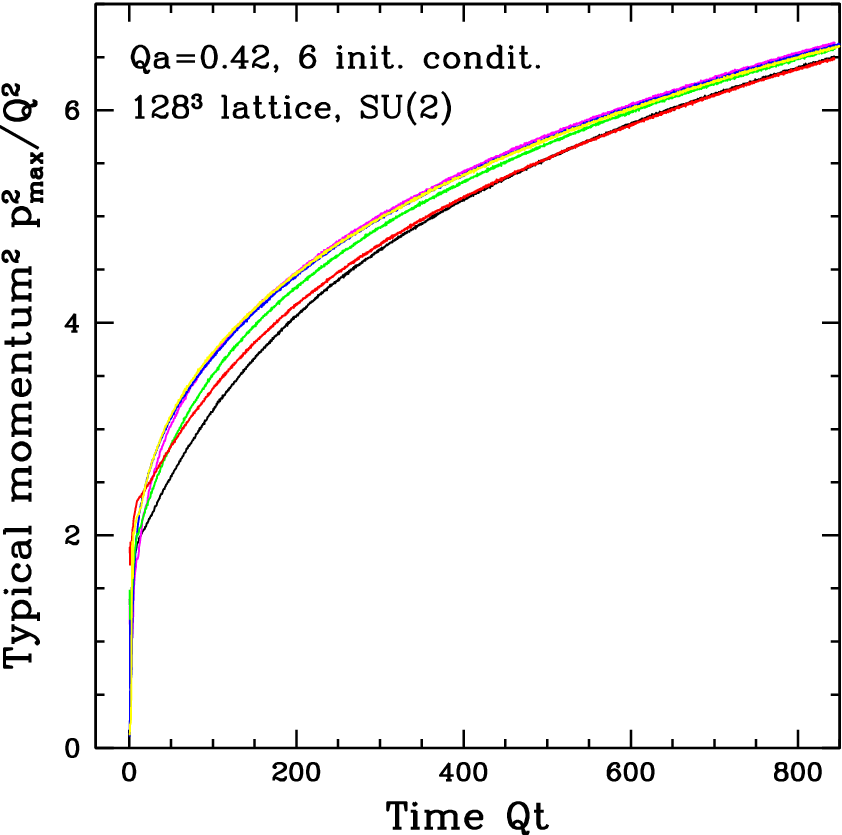
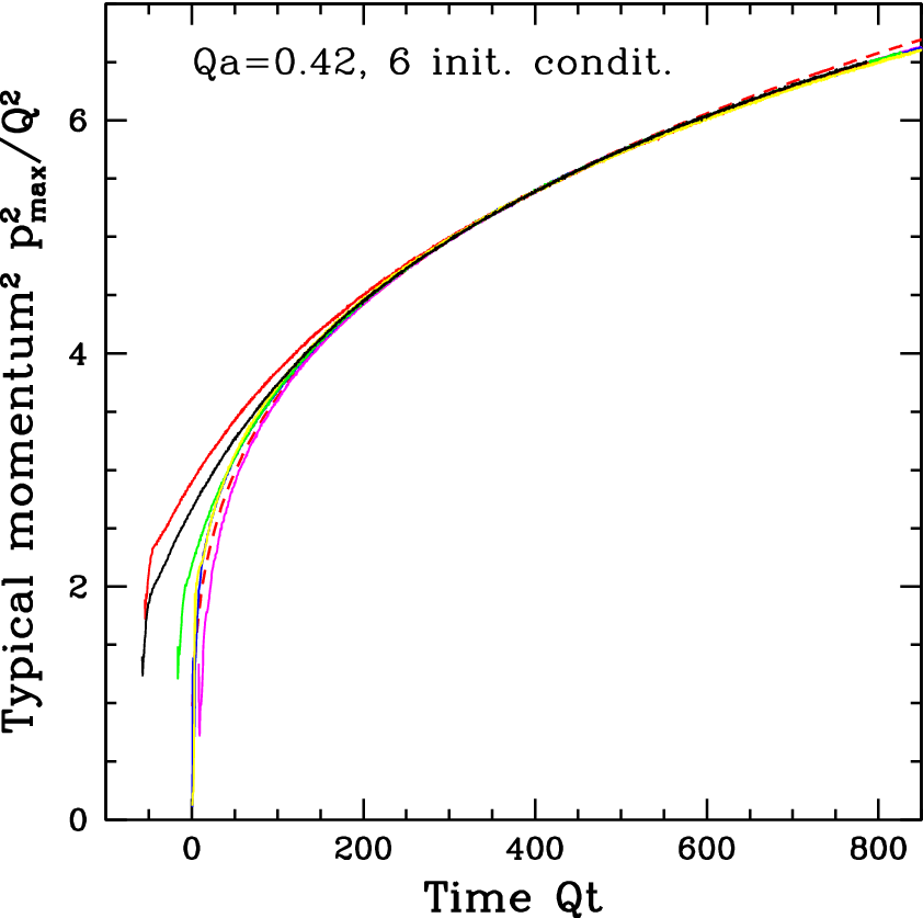
The simplest gauge invariant measurable is defined in Eq. (12). So to examine the approach to scaling we will first look at results for this quantity. To do so we created several different initial conditions, with either infrared electric fields, magnetic fields, or both present, and with different ranges of momenta occupied. To keep lattice systematics common, they all have approximately the same value of , namely . The evolution behavior of as a function of is shown for 6 initial conditions in Figure 1. Each curve shows an initial transient, whose length depends on the initial condition; but after some time they all approach a common scaling behavior. In the lefthand figure the time is based on the starting time of the simulation; but depending on the initial condition, there may be a delay before the dynamics starts to track towards the scaling solution (or it may reach the scaling solution early, if the initial condition is already quite similar). Therefore, to understand whether the evolution really approaches a scaling solution, it makes more sense to shift each initial time so that the curves are more similar at late time. We have done so in the righthand figure, which shows that the different initial conditions very accurately fall onto the same scaling behavior. The red dotted line is a 1-parameter fit, , which shows that the curves are obeying the expected time scaling. Unfortunately, by the scale has already reached , which means that lattice spacing errors start to occur; at we expect of order errors due to higher-dimension operators in the lattice action. So precision quantitative results would demand a finer lattice (smaller ).
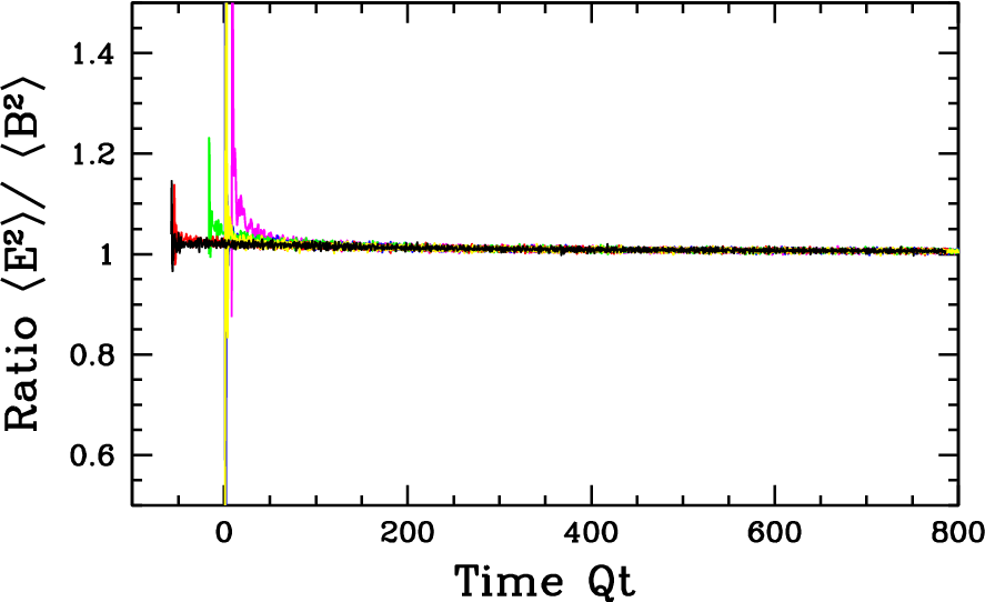
We can also look at the gauge invariant ratio of electric to magnetic energy densities , shown in Figure 2. A quasiparticle with momentum large compared to the plasma frequency should have equal time-averaged electric and magnetic energy. Plasmons with would display more electric than magnetic energy, whereas magnetic fields in this regime (the Landau cut) would have more magnetic energy. So a condensate of plasmon quasiparticles would be expected to manifest as an excess of electric field energy leading to a ratio larger than 1, while a condensate of magnetic field would give a ratio smaller than 1. In fact, after a short and initial-condition dependent transient, the ratio settles down to be close to but slightly above 1, decaying towards 1 with time.55 5 Specifically, in the figure, the blue curve has initial conditions with purely electric energy; the yellow curve has purely magnetic energy. The other curves have a mix of electric and magnetic but in different momentum ranges. This suggests against the existence of large condensates; but we will examine the evidence in more detail in the next section.
3.1 Gauge fixed observables
To learn more about the evolving configurations on the lattice, it is useful to examine gauge-fixed observables. Coulomb gauge is the choice of gauge which minimizes . It is therefore perhaps the most sensible gauge to use for studying the distribution of excitations at one moment in time. And the technology for fixing to Coulomb gauge on the lattice is very well known, amounting to the fixing of Landau gauge for the 3-D configuration at an instant [10]. Since the gauge fixing procedure emphasizes minimizing at every time at the expense of minimizing , unequal time correlators in this gauge tend to have very short autocorrelation. So we will not attempt to untangle unequal time correlations using gauge fixed methods.
Conventionally, one uses the perturbative relation between occupancy and field amplitude, for transverse quasiparticle excitations,
| (13) | |||||
| (14) |
(with the transverse projector), to estimate the occupancies as
| (15) | |||||
| (16) |
In this way we obtain two estimates of the occupancies, one from gauge fields and one from electric fields. To illustrate the utility, and the danger, of this approach, we use it to examine the occupancies of a nonperturbative lattice system in equilibrium.66 6 The lattice system has an equilibrium because the available momenta are restricted to a Brillouin zone, so the phase space is finite. From the point of view of continuum classical field theory, this equilibrium state is a complete lattice artifact. In equilibrium one usually expects , which is small provided . To ensure that the occupancy is small for typical lattice momenta , we consider a lattice with spacing (which is in the conventional lattice notation). The results for the occupancies and are shown in Figure 3.
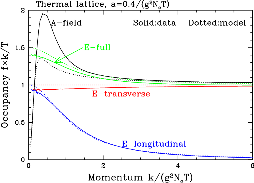
The figure shows and as the black and green curves. But whereas the -field is automatically transverse because of our gauge condition, the electric field is not. Gauss’s law states , not , and below the Debye scale the two become strongly inequivalent. Therefore we have separately plotted the transverse electric estimator
| (17) |
and the longitudinal electric estimator
| (18) |
At the level of hard thermal loops these have simple expressions (see Appendix A)
| (19) |
The estimator is , which therefore systematically rises at small momenta . Physically, the reason rises is that, for , there are three polarization states contributing to the electric field correlator, but the estimator Eq. (16) assumes that there are only two. Therefore, below the scale , the estimator is incorrectly normalized and systematically high. However the estimator is based on a correct counting of degrees of freedom and should be used instead.
The figure also shows that the -field correlator does not reproduce the expected behavior . As one goes down in momentum scale , it first rises above the leading-order estimate, peaks, and falls to zero at small momentum. The rise is due to perturbative corrections to the correlator, which are known; at next-to-leading order,
| (20) |
Note that the first correction is suppressed by , not by . The dotted “model” curve shown in Figure 3 uses the above correlator with replaced with , which seems to match the infrared behavior. The “model” curves for the curves are based on Eq. (19) and the lowest-order lattice value for , [11]
| (21) |
Because rises above the leading-order expectation, using to estimate provides a systematic over-estimate; for the lattice we considered, it over-estimates the actual magnetic energy by 3.5%. But gets the electric energy exactly right. With these remarks in mind, we will use to estimate the occupancy and will use as a secondary estimator, with some caution about the meaning of its infrared behavior.
3.2 Approach to scaling
We have performed a number of classical gauge field evolutions on lattices of size up to and for times in excess of . Provided that we concentrate on that part of an evolution where , we consistently see the approach to scaling expected from our kinetic theory study. To illustrate this, Figure 4 shows versus at a number of times, first in absolute units and then building in the assumption of scaling as described in Eq. (10) and Eq. (11). We see that, after rescaling and to remove their dominant time scaling, the occupancy takes the same form quite accurately over a wide range of times.


How quickly do the gauge fields approach this scaling solution? To study this, we look at the same initial conditions used in Figure 1. Figure 5 shows the occupancies and , starting at an early time where the very different initial conditions are evident and continuing until they have approached a common behavior. The spectra agree at the same time that the values of converge in Figure 1, of order .
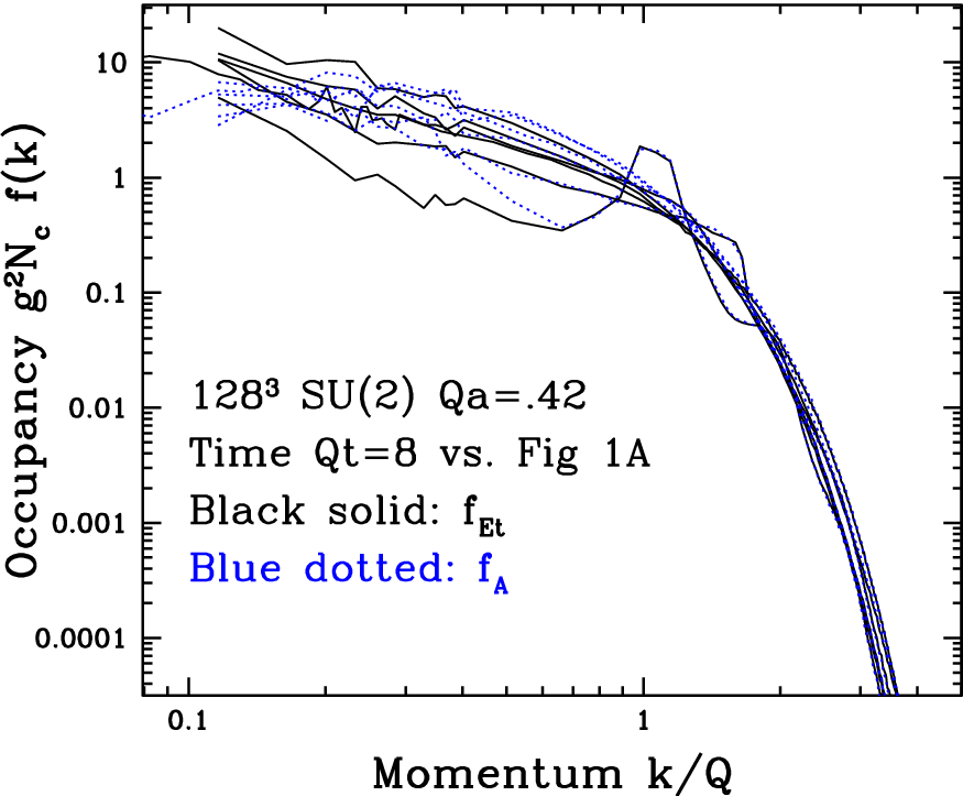
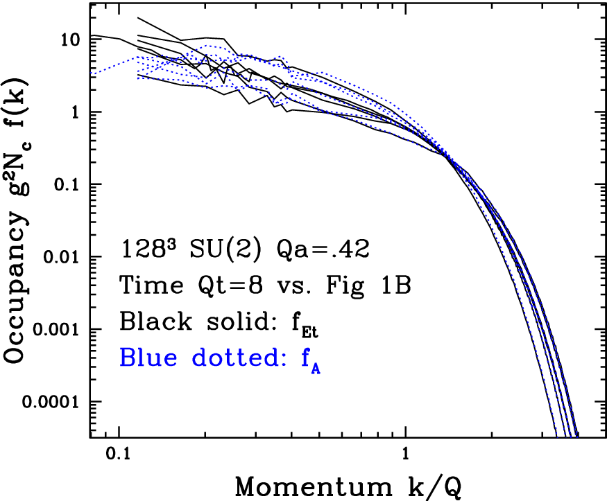
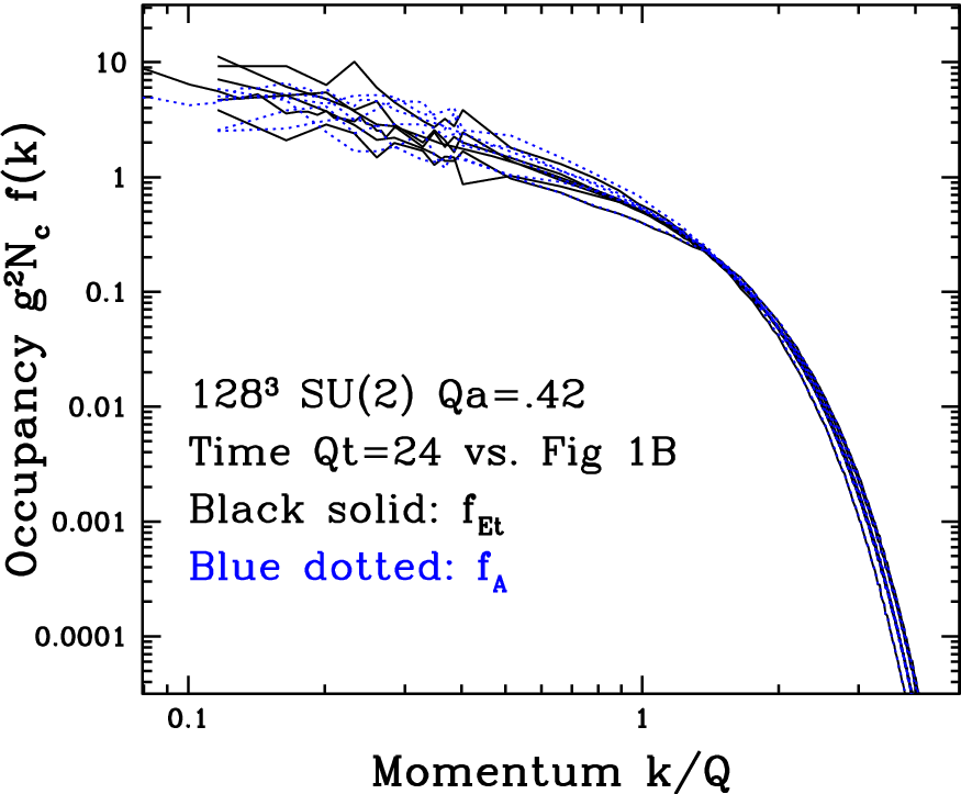
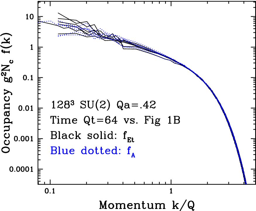
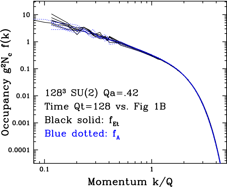
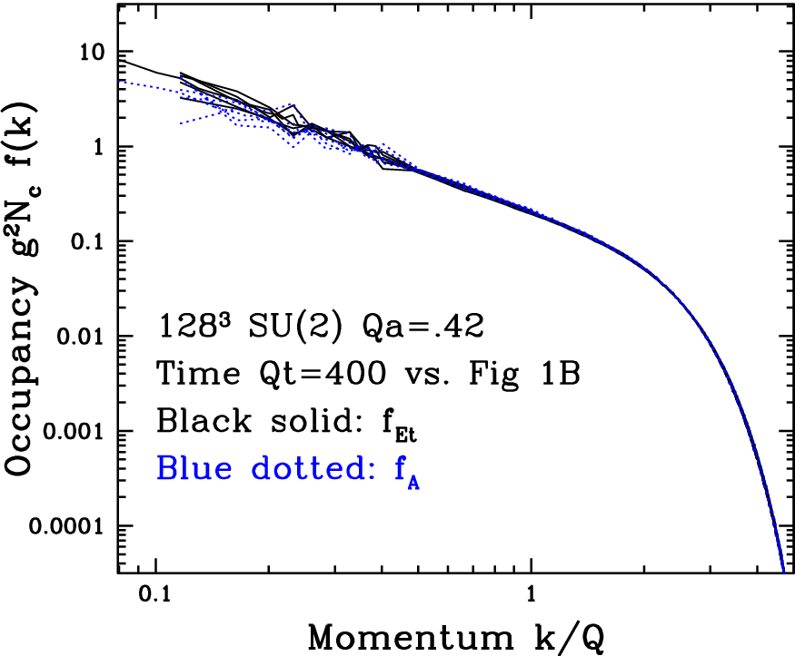
Looking at Figure 4 and Figure 5, it appears that the scaling solution is not completely time independent, but shows some weak time evolution. First, the large-momentum, low-occupancy falloff appears to evolve with time. Second, the infrared behavior, below the characteristic scale , also shows some evolution. The evolution at low momentum is real and we will look at it in more detail in the next subsection. But the evolution at large momentum is a lattice artifact, caused by higher dimension operators which become important at momentum scales . To illustrate this, we plot the UV falloff at several times and lattice spacings in Figure 6. The figure shows clearly that the differences between curves are associated with their taking different values of , not with their being at different times .77 7 We should clarify that the momentum in the figure is really the square root of the free lattice dispersion , which for our Wilson lattice action is .

3.3 Evolution of the scaling solution
Now we examine in more detail whether there is time evolution in the infrared part of the scaling solution. We saw in Figure 5 that distinct initial conditions approach a common scaling solution by . Our focus will be on time scales this long or longer. To do so we performed several independent evolutions on large () and relatively coarse () lattices, averaging and obtaining ensemble error bars. For times longer than we also performed simulations at .


The results are displayed in Figure 7. The figure first compares (black solid lines) to (blue dashed lines), in the top two figures. To test for a infrared scaling behavior, we have multiplied the occupancies by and plotted in the figure.
The lower right plot focuses on . It shows that scales as from about out to the infrared scale where the occupancy hits the value , indicated by the red dashed lines. Then it saturates at this value. The value is the same as the maximum value we found in the equilibrium study, so this appears to indicate that the occupancy has become nonperturbatively large and encountered magnetic screening. We can estimate the total particle number in nonperturbative infrared magnetic fields by integrating starting where . We find that the fraction of particle number in the condensate,
| (22) |
is , , , , and for , 72, 156, 299, and 544 respectively.
Now consider the electric occupancies. The lower left figure compares with . It also presents an estimate of the Debye screening scale, obtained by evaluating
| (23) |
the quantity which would perturbatively give . This determination of is indicated for each evolution by a (magenta) vertical bar, with the rightmost (large-) bar representing the earliest time and the leftmost (small-) bar the latest time. As we have seen, is the scale where we would expect and to start differing from each other significantly, and this is indeed the case. Since is established assuming there are only two occupied polarizations, while below there are really three, it is which should be used as an estimate of occupancy. The fact that rises above could lead to an incorrect inference that at least the electric occupancies rise more steeply than in the infrared. In fact rises in the IR for , but not as strongly as we would find using .
The use of to estimate occupancies is also not really correct below the scale , because Eq. (14) and Eq. (16) assume free dispersion of plasmons, while the plasmon dispersion is strongly modified in this region; the factor in Eq. (16) should presumably be replaced by . (This is also not quite right because part of the electric field strength resides in the Landau cut. We have no good way of separating the pole and cut contributions, but for one expects the pole (plasmon) contribution to dominate, so we will ignore this complication.) If we bravely redefine as
| (24) |
and re-plot just against , we get the occupancies shown in Figure 8. (The figure adds two lines at later times obtained on a finer lattice with .)

What Figure 8 shows is that the apparent rise in , found in Figure 7, arose because the occupancies were being mis-evaluated, not taking into account the dispersion of the plasmons which is describing. When one takes this into account, one finds for that there is a clean scaling window with scaling behavior, and then a falloff at momenta below the plasma frequency.
In summary, as increases, a scaling window opens between the scale and an infrared scale where occupancies become nonperturbatively large and the physics of plasmons is important. This scaling window shows . After correctly identifying the relation between electric field correlators and occupancy, we find no evidence for scaling at any time.
4 Are there condensates?
Recently Blaizot et al have argued that the evolution of classical Yang-Mills theory, of precisely the sort considered here, may lead to the formation of condensates of gluons in the deep infrared [4]. If by condensate one means that the occupancy reaches the scale in the infrared, then we definitely see a condensate.88 8 Using this definition, there is also a condensate in weakly coupled Yang-Mills theory in equilibrium. As discussed above, we find that
| (25) |
which is easily solved for the scale where :
| (26) |
The occupancy integrated at and below this scale is of order . Therefore the particle number stored in the condensate decays with time as the power of time. Relative to the total particle number, which scales as , the condensate makes up a fraction of particle number which scales as . Using the estimates for magnetic particle number with in the last section, we find the data fit this trend well, with a prefactor of about 0.45 – that is, if we define as “condensate” any modes with occupancy , we find the condensate makes up of the total particle number.
We do not see evidence for a time-independent or long-lived transient population of occupancy modes in excess of the time-scaling estimate above. We also do not see evidence for a more robustly-defined condensate, in which the occupancy in a very narrow momentum range exceeds . We believe that such an condensate is physically possible for plasmons, but happens not to occur; and that it is very difficult for such a condensate even to occur in magnetic fields. We will present both of these arguments in more detail in this section.
4.1 Electric condensates: decay rate of plasmons
One possibility is the development of a condensate of plasmons, which are the low momentum extension of the conventional quasiparticles. Is there any evidence for such a condensate in the preceding results on occupancies? To answer this question, we think it is useful to see what a condensate of plasmons would look like and how it would evolve. We can do so by artificially introducing a condensate of plasmons into a classical simulation during the cascade towards the ultraviolet, examining it with the tools of the previous section.
With this in mind, we have performed three simulations with on lattices in which we stop the evolution at some point in time, fix to Coulomb gauge, add a perfectly spatially uniform electric field, re-enforce Gauss’ Law99 9 Gauss’ Law is that . A uniform electric field in Coulomb gauge satisfies , which is not the same; therefore the configuration where a uniform field has been added will not satisfy Gauss’ Law. We enforce Gauss’ Law by projecting to the Gauss constraint using the algorithm of Ref. [12]., and then follow the evolution. We performed three runs, introducing the electric field at times , , and .
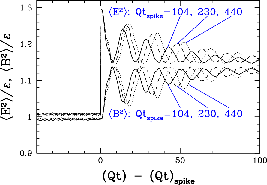
Figure 9 plots the electric and magnetic energy as a function of time after the introduction of the IR electric field. Unsurprisingly, the electric field energy jumps up at the moment when we add the coherent -field. The electric field energy then oscillates between an almost equal division with magnetic energy and an excess of electric energy. These are plasma oscillations. In a plasma oscillation, energy goes back and forth between the electric field and a coherent motion of the charged quasiparticles. Since quasiparticles have almost equal electric and magnetic energy, when the plasmon is stored in quasiparticles, . The time between maxima (or between minima) of the electric field energy is . We can estimate by using and getting from Eq. (23), or we can read directly off the plot; the two agree at the level. In particular it is clear that is smaller at later times.
The amplitude of the oscillations in -field energy decay with time. This indicates that the plasmons are either scattered to other momenta, or absorbed by number-changing processes.1010 10 If the plasmons were scattered to momenta differing by from the original value, they would lose phase coherence with the plasmon, but would continue to have a time-averaged . This would prevent the maxima in from almost reaching the minima. But we observe that they continue to almost meet; so we believe the plasmon damping is dominated by absorption and scattering to momenta . The occupancy falls by about a factor of 2 in one plasma oscillation ( or two peaks), with the decay occurring faster for the system where we introduced the -condensate at an earlier . The time scale for plasmon decay is short compared to the system age for all of the cases we considered. Therefore we conclude that a condensate of plasmons would be short-lived; at any time, any plasmons must be of recent origin rather than quanta left over from the initial conditions.


We have also investigated the occupancies and when this large plasmon condensate is present. Figure 10 shows the occupancies for our simulation at two points during the plasmon oscillations: when the -field energy has its first minimum and all energy is in quasiparticles (left), and when the -field has its next maximum and the energy is in an -field condensate (right). The dotted lines in the figure are the occupancies at the same time but in a simulation where the -field spike is not added, for comparison. The figure shows that, when , the plasmon energy is stored in a redistribution of the quasiparticles. When has its peak, there is a condensate of soft -fields, with the occupancy reaching 3 orders of magnitude higher than without the plasmon condensate. This is a real condensate! By comparison, we can conclude that there is not a condensate of plasmons in the normal simulation.
What this investigation shows is that a condensate of plasmons is possible in principle. In particular, an intense and uniform -field does not create an exponential instability and break up in a time scale [13]. Instead, such a condensate oscillates between manifesting as an -field and as a coherent motion of partons. (Note that the right graph in Figure 10 is at a time after the left graph in the figure, and shows that a large -field occupancy regenerates from the coherent motion of quasiparticles.)
The evidence for such a condensate in an ordinary simulation would come in two parts; an excess of electric over magnetic energy, and a spike in the small- occupancy . A slight excess of over is observed, but it is already below for and it decays thereafter. Also, such an excess is expected because of ordinary perturbative interactions, which should lead to an excess of order (the scaling we observe). We also definitely do not observe an infrared spike in , as shown in Figure 7 and Figure 8. So while an electric or plasmon condensate is possible, we do not see one.
4.2 Magnetic condensates: Nielsen-Olesen instabilities
What about condensates in the magnetic sector? We will argue here that such condensates are difficult to define or identify in Coulomb gauge. But we will also show that genuine condensates, in the sense of magnetic field occupancies greatly in excess of for a narrow range of -vectors, are highly unstable in a nonabelian theory.

First we explain why it is difficult for magnetic occupancies to be highly coherent in the sense of occupancies exceeding , or equivalently . Suppose that there is a gauge field configuration with infrared fields of size , with some length scale. Consider Figure 11 and ask if the field can be coherent between points , and , separated by distances of order . We might say that the field at and at are “the same” if the parallel transport of the field at , along the path , is the same or similar to the field at . Similarly, the field is the same between and if parallel transported along path is the same as . But because the field is large, the Wilson line along and then will differ by an order-1 group element from the Wilson line along – roughly, by times the flux of field going through the loop, which is order 1. Therefore, the parallel transport of the field at , first along path and then along path , cannot agree with the same field parallel transported just along path . So a comparison of the field at and at , using the path , will show that they are very different. Therefore there is no sense that the field is really coherent on scales as large as or larger than .
Since there is no gauge invariant sense in which a gauge field of amplitude can be coherent on scales , it would be surprising – and probably just a gauge choice artifact – for to be coherent on longer scales. When a field is random over scales longer than , its Fourier transform has roughly uniform power over momenta less than . If the real-space field strength is and this is distributed over Fourier modes with , then the Fourier-space correlator will be , corresponding to an occupancy for (see Eq. (13)).
A loophole in the above reasoning is the case where points in the same color direction throughout a large region of space – that is, if happens to be approximately abelian (or more generally, if commutes with the field strength through any arbitrary Wilson loop). This is very nongeneric, since is specified by numbers (each color can point in a different space direction), but a gauge transformation contains only independent elements. Therefore elements of must coincidentally vanish for it to be nearly abelian. Nevertheless it is useful to consider what happens in this special case, where there certainly can be coherence on large scales. So consider the case where only the component of is nonzero, and is uniform in space. It is quite easy to consider this possibility on the lattice, and we have done so, adding roundoff error sized fluctuations in other field modes. We observe the exponential growth of electric field fluctuations; we plot and as a function of in Figure 12, and and as a function of at a series of times in Figure 13. (In both figures we set the zero of time to the first moment when .) Figure 12 shows that the electric field energy grows exponentially until it actually exceeds the magnetic energy; then there are brief, highly damped oscillations, ending in an almost equal energy partition between and . The lefthand plot of Figure 13 shows occupancies during the process of electric field growth, with successive curves at successive times separated by about . The righthand plot shows the process of field saturation at a series of times around . The figure shows that the magnetic condensate (the spike at the earliest time) disappears; then there is some chaotic dynamics with a very short-lived high IR occupancy of electric fields. But these fields are mostly gone by , when the configuration already resembles the occupancies during the cascade.


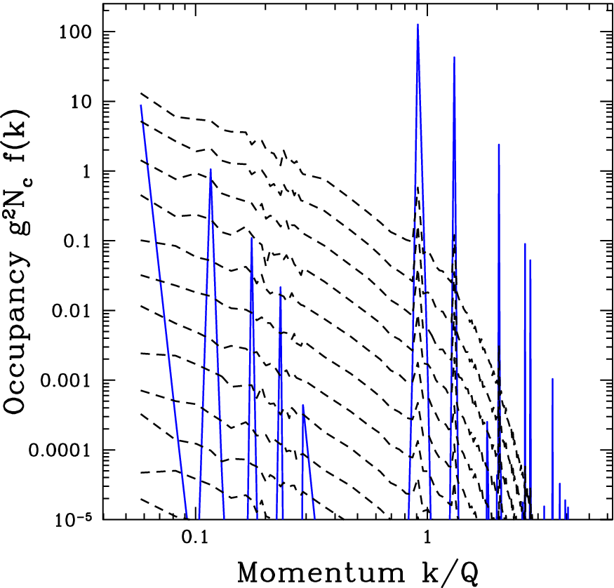
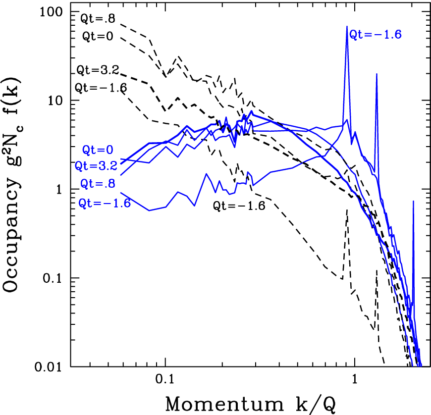
The reason for the exponential growth of electric fields in the presence of a uniform field is the Nielsen-Olesen instability. As shown by Nielsen and Olesen [14], in a uniform field there are modes whose amplitude will grow at the rate1111 11 Here is a lightning quick derivation of this result. In the presence of a magnetic field, charges follow Lamor orbits, causing transverse momentum to be quantized, , with the Landau level. The energy of an excitation is , with spin-magnetic interaction term. For a spin-1 particle, depending on polarization. The minimum of is obtained when , and . In this case the energy is , corresponding to exponential growth with exponent .
| (27) |
The occupancy and energy go as and grow at twice this rate. This is precisely the growth rate we observe. The arguments of Nielsen and Olesen apply whenever the magnetic field is coherent over a distance scale large compared to . This essentially forbids magnetic fields with such coherence as to have ; any such magnetic field would be exponentially unstable and rapidly dissolve.
A curious feature of Figure 13 is that, even though we started with a perfectly uniform and abelian gauge field configuration, the process of finding Coulomb gauge has interpreted it as a nonuniform and nonabelian configuration; the occupancy in Figure 13 has its peak at rather than at . It is still recognizable as a condensate; using our former definition that “condensate” means , we find about of the particle number is in a condensate. The fact that the field is highly coherent is stored in the very peculiar structure of the inferred occupancies, with a sharp spike reaching far above , the limit we have observed in thermal and stochastic cascading systems. We believe that a genuine magnetic condensate would appear as a similar, structured and sharp feature in the magnetic occupancy – a feature which does not appear at any point in our simulations except those which start with a coherent -field.
To summarize, we directly observe the Nielsen-Olesen instability; whenever the magnetic field is coherent on a scale larger than the Lamor radius of charges in the field, , there are exponentially unstable modes, growing on a time scale , which consume the -field and turn into a stochastic collection of excitations. This physics should prevent fields with , corresponding to occupancies larger than roughly .
5 Discussion
Classical Yang-Mills theory, initially occupied in the infrared, sees a cascade of energy towards the ultraviolet, due to the infinite phase space available there. Simple arguments, which suggest and , are borne out, and in fact, scaling out this dominant behavior, we find that the occupancy rapidly approaches a scaling solution.
The infrared dynamics at intermediate times () are complicated because the screening and nonperturbative scales are not well separated from the scale . At the scale the electric field takes on significant longitudinal occupancy, and one should use only its transverse components to estimate the quasiparticle occupancy, to avoid miscounting. Below around the dispersion of plasmons should also be considered. Taking these effects into account, we find no evidence for scaling; when any scaling window exists in the infrared, it always shows exponent . The occupancy determined from -field correlators agrees with that from -field correlators until around the scale , where they start to diverge. The magnetic occupancy saturates at about , and the total particle number in such nonperturbatively large fields (magnetic condensate) scales with time as .
It is possible for electric (plasmon) condensates to exist; indeed, we can artificially introduce them into a lattice evolution to investigate their behavior. The plasmons can carry occupancy large compared to , but in practice they do not. And the damping rate for plasmons is fast compared to the system’s age.
Genuine magnetic condensates are unstable due to the Nielsen-Olesen instability; we verify the growth rate of fluctuations in the presence of a perfectly coherent -field, . The high-occupancy infrared magnetic field observed during the scaling cascade to the ultraviolet better resembles the nonperturbative incoherent -fields in equilibrium weakly-coupled Yang-Mills theory.
It would be interesting to solve the Boltzmann equations for Yang-Mills theory, presented in Reference [7], directly, to compare against the numerical scaling solution found here.
Acknowledgments
We would like to thank Kari Rummukainen and Mark York for collaboration during the early stages which lead to this paper, and Jürgen Berges, Sören Schlichting, Francois Gelis, and Raju Venugopalan for conversations. We also thank the Department of Energy’s Institute for Nuclear Theory at the University of Washington for providing the engaging environment in which this work was started. This work was supported in part by the Canadian National Sciences and Engineering Research Council (NSERC) and the Institute of Particle Physics (Canada). Part of the computational work was performed at the Finnish IT Center for Science (CSC), Espoo, Finland.
Appendix A Equilibrium -field correlators
Consider classical Yang-Mills theory with some UV regulator (such as the lattice). Because the theory is UV regulated it has a well defined thermal ensemble, described by the path integral
| (28) |
The delta function enforcing Gauss’ Law is a functional delta, with one such delta at each point. We can rewrite it in terms of a Lagrange multiplier, suggestively named [15]:
| (29) |
If we perform the Gaussian integration over the -field we obtain
| (30) |
the standard bare kinetic term for the field. Under renormalization this mixes with the identity, generating the Debye mass [11]:
| (31) |
But this IR behavior should already hold even if we don’t integrate out the -field. In the infrared, the behavior of is
| (32) |
Now we can integrate out the field,
| (33) |
neglect the difference between and , and use this to evaluate the transverse and longitudinal -field correlators:
| (34) | |||||
| (35) |
Combining with Eq. (17) and Eq. (18), Eq. (19) follows. The sum rule is not exact because we have approximated with ; but our numerical results in Figure 3 show that it is surprisingly accurate.
References
- [1] See for instance, L. D. McLerran, R. Venugopalan, Phys. Rev. D49, 2233-2241 (1994). [arXiv:hep-ph/9309289 [hep-ph]]; Phys. Rev. D49, 3352-3355 (1994) [hep-ph/9311205]; A. Kovner, L. D. McLerran, H. Weigert, Phys. Rev. D52, 6231-6237 (1995) [hep-ph/9502289]; or for recent reviews, E. Iancu, R. Venugopalan, In *Hwa, R.C. (ed) et al.: Quark gluon plasma* 249-3363 [hep-ph/0303204]; F. Gelis, E. Iancu, J. Jalilian-Marian and R. Venugopalan, Ann. Rev. Nucl. Part. Sci. 60, 463 (2010) [arXiv:1002.0333 [hep-ph]].
- [2] A. Kurkela and G. D. Moore, JHEP 1112, 044 (2011) [arXiv:1107.5050 [hep-ph]].
- [3] R. Micha and I. I. Tkachev, Phys. Rev. D 70, 043538 (2004) [hep-ph/0403101].
- [4] J. -P. Blaizot, F. Gelis, J. -F. Liao, L. McLerran and R. Venugopalan, Nucl. Phys. A 873, 68 (2012) [arXiv:1107.5296 [hep-ph]].
- [5] J. Berges, S. Schlichting and D. Sexty, arXiv:1203.4646 [hep-ph].
- [6] J. Berges, S. Scheffler and D. Sexty, Phys. Lett. B 681, 362 (2009) [arXiv:0811.4293 [hep-ph]].
- [7] P. B. Arnold, G. D. Moore and L. G. Yaffe, JHEP 0301, 030 (2003) [hep-ph/0209353].
- [8] J. Berges and D. Sexty, Phys. Rev. Lett. 108, 161601 (2012) [arXiv:1201.0687 [hep-ph]].
- [9] J. Ambjørn, T. Askgaard, H. Porter and M. E. Shaposhnikov, Nucl. Phys. B 353, 346 (1991).
- [10] J. E. Mandula and M. Ogilvie, Phys. Lett. B 185, 127 (1987).
- [11] K. Kajantie, K. Rummukainen and M. E. Shaposhnikov, Nucl. Phys. B 407, 356 (1993) [hep-ph/9305345]; K. Kajantie, M. Laine, K. Rummukainen and M. E. Shaposhnikov, Nucl. Phys. B 458, 90 (1996) [hep-ph/9508379].
- [12] Guy D. Moore, Nucl. Phys. B 480, 657 (1996) [hep-ph/9603384].
- [13] Contrary to what one of us (GDM) has claimed in discussions on some recent occasions.
- [14] N. K. Nielsen and P. Olesen, Nucl. Phys. B 144, 376 (1978).
- [15] J. Ambjørn and A. Krasnitz, Phys. Lett. B 362, 97 (1995) [hep-ph/9508202].