Controllers with Minimal Observation Power
(Application to Timed Systems) Thanks: Partly supported by ANR project ECSPER (JC09- 472677), ERC Starting Grant inVEST-279499, Danish-Chinese Center for Cyber Physical Systems (IDEA4CPS) and VKR Center of Excellence MT-LAB.

A run of a LTS is a finite or infinite sequence of states $r=(s_{0},s_{1},\dots,s_{n},\dots)$ such that $s_{i}\xrightarrow{a_{i}}s_{i+1}$ for some action $a_{i}\in\Sigma$. $r^{i}$ denotes the prefix run of $r$ ending at $s_{i}$. We denote by $Runs(A)$ the set of all finite runs of the LTS $A$ and by $Runs^{\omega}(A)$ the set of all infinite runs of the LTS $A$.

A state predicate is a characteristic function $\varphi:S\rightarrow\{0,1\}$. We write $s\models\varphi$ iff $\varphi(s)=1$.

We use LTS as arenas for games: at each round of the game Player I (Controller) chooses an action $a\in\Sigma$, and Player II (Environment) resolves the nondeterminism by choosing a transition labeled with $a$. Starting from the state $s_{init}$, the two players play for an infinite number of rounds, and this interaction produces an infinite run that we call the outcome of the game. The objective of Player I is to keep the game in states that satisfy a state predicate $\varphi$, this predicate typically models the safe states of the system.

More formally, Player I plays according to a strategy $\lambda$ (of Player I) which is a mapping from the set of finite runs to the set of actions, i.e. $\lambda:Runs(A)\rightarrow\Sigma$. We say that an infinite run $r=(s_{0},s_{1},s_{2},\dots,s_{n},\dots)\in Runs^{\omega}(A)$ is consistent with the strategy $\lambda$, if for all $0\leq i$, there exists a transition $s_{i}\xrightarrow{\lambda(r^{i})}s_{i+1}$. We denote by ${\sf Outcome}(A,\lambda)$ all the infinite runs in $A$ that are consistent with $\lambda$ and start in $s_{init}$. An infinite run $(s_{0},s_{1},\dots,s_{n},\dots)$ satisfies a state predicate $\varphi$ if for all $i\geq 0$, $s_{i}\models\varphi$. A (perfect information) safety game between Player I and Player II is defined by a pair $(A,\varphi)$, where $A$ is an LTS and $\varphi$ is a state predicate that we call a safety state predicate. The safety game problem asks to determine, given a game $(A,\varphi)$, if there exists a strategy $\lambda$ for Player I such that all the infinite runs in ${\sf Outcome}(A,\lambda)$ satisfy $\varphi$.

In the imperfect information setting, Player I observes the state of the game using a set of observable predicates $obs=\{\varphi_{1},\varphi_{2},\dots,\varphi_{m}\}$. An observation is a valuation for the predicates in $obs$, i.e. in a state $s$, Player I is given the subset of observable predicates that are satisfied in that state. This is defined by the function $\gamma_{obs}$:

We extend the function $\gamma_{obs}$ to sets of states that satisfy the same set of observation predicates. So, if all the elements of some set of states $v\subseteq S$ satisfy the same set of observable predicates $o$ (i.e. $\forall s\in v\cdot\gamma_{obs}(s)=o$), then we let $\gamma_{obs}(v)=o$.

In a game with imperfect information, Player I has to play according to observation based stuttering invariant strategies (OBSI strategies for short). Initially, and whenever the current observation of the system state changes, Player I proposes some action $a\in\Sigma$ and this intuitively means that he wants to play the action $a$ whenever this action is enabled in the system. Player I is not allowed to change his choice as long as the current observation remains the same.

An Imperfect Information Safety Game (IISG) is defined by a triple $(A,\varphi,obs)$.

Consider a run $r=(s_{0},s_{1},\dots,s_{n})$, and its prefix $r^{\prime}$ that contains all the elements but the last one (i.e. $r=r^{\prime}\cdot s_{n}$). A stuttering-free projection $r\downarrow obs$ of a run $r$ over a set of predicates $obs$ is a sequence, defined by the following inductive rules:

• •

  if $r$ is a singleton (i.e. $n=0$), then $r\downarrow obs=\gamma_{obs}(s_{0})$

• •

  else if $n>0$ and $\gamma_{obs}(s_{n-1})=\gamma_{obs}(s_{n})$, then $r\downarrow obs=r^{\prime}\downarrow obs$

• •

  else if $n>0$ and $\gamma_{obs}(s_{n-1})\neq\gamma_{obs}(s_{n})$, then $r\downarrow obs=r^{\prime}\downarrow obs\cdot\gamma_{obs}(s_{n})$

We say that Player I wins in IISG $(A,\varphi,obs)$, if there exists a $obs$-OBSI strategy $\lambda$ for Player I such that all the infinite runs in ${\sf Outcome}(A,\lambda)$ satisfy $\varphi$.

The solution of a IISG $(A,\varphi,obs)$ can be reduced to the solution of a perfect information safety game $(G,\psi)$, whose states are sets of states in $A$ and represent the knowledge (beliefs) of Player I about the current possible states of $A$.

We assume that $\varphi\in obs$, i.e. the safety state predicate is observable for Player I. This is a reasonable assumption since Player I should be able to know whether he loses the game or not.

Consider an LTS $A=(S,s_{init},\Sigma,\rightarrow)$. We say that a transition $s_{1}\xrightarrow{a}s_{2}$ in $A$ is $obs$-visible, if the states $s_{1}$ and $s_{2}$ have different observations (i.e. $\gamma_{obs}(s_{1})\neq\gamma_{obs}(s_{2})$), otherwise we call this transition to be $obs$-invisible. Let $v\subseteq S$ be a knowledge (belief) of Player I in $A$, i.e. it is some set of states that satisfy the same observation. The set $Post_{obs}(v,a)$ contains all the states that are accessible from the states of $v$ by a finite sequence of $a$-labeled $obs$-invisible transitions followed by an $a$-labeled $obs$-visible transition. More formally, $Post_{obs}(v,a)$ contains all the states $s^{\prime}$, such that there exists a run $s_{1}\xrightarrow{a}s_{2}\xrightarrow{a}\dots\xrightarrow{a}s_{n}$ and $s_{1}\in v$, $s_{n}=s^{\prime}$, $\gamma_{obs}(s_{i})=\gamma_{obs}(s)$ for all $1\leq i<n$, and $\gamma_{obs}(s_{n})\neq\gamma_{obs}(s)$.

The set $Post_{obs}(v,a)$ contains all the states that are visible for Player I after he continuously offers to play action $a$ from some state in $v$. Player I can distinguish the states $s_{1}$ and $s_{2}$ from $Post_{obs}(v,a)$ iff they have different observations, i.e. $\gamma_{obs}(s_{1})\neq\gamma_{obs}(s_{2})$. In other words, the set $\{Post_{obs}(v,a)\cap\gamma_{obs}^{-1}(o)\mid o\in{\mathcal{P}}(obs)\}\setminus\{\varnothing\}$ consists of all the beliefs that Player I might have after he plays the $a$ action from the knowledge set $v$¹¹ 1 the powerset ${\mathcal{P}}(S)$ is equal to the set of all subsets of $S$.

A game can diverge in the current observation after playing some action. To capture this we define the boolean function $Sink_{obs}(v,a)$ whose value is true iff there exists an infinite run $(s_{0},s_{1},\dots,s_{n},\dots)\in Runs(A)$ such that $s_{0}\in v$ and for each $i\geq 0$ we have $s_{i}\xrightarrow{a}s_{i+1}$ and $\gamma_{obs}(s_{i})=\gamma_{obs}(s_{0})$.

This theorem gives us the algorithm of solution of a IISG for the case when the knowledge games for it is finite and can be automatically constructed.

Consider, that we already solved the game for the observable predicates sets $obs_{1},obs_{2},\dots,obs_{n}$ and obtained the results $r_{1},r_{2},\dots,r_{n}$, where $r_{i}$ is either $true$ or $false$, depending on whether Player I wins in IISTG $(M,\varphi,obs_{i})$ or not.

From now on we don’t have to consider any set of observable predicates with a cost larger or equal to the cost of the optimal solution found so far. Additionally, if we know, that Player I loses for the set of observable predicates $obs_{i}$ (i.e. $r_{i}=false$), then we can conclude that he also loses for any coarser set of observable predicates $obs\subset obs_{i}$ (since in this case Player I has less observation power). Therefore we don’t have to consider such $obs$ as a solution to our optimization problem. This can be formalized by the following definition:

Algorithm 1 solves the optimization problem by iteratively solving the game for different sets of observable predicates so that the resulting sequence of solutions is non-redundant. The procedure $Solve(M,\varphi,obs)$ uses the knowledge game-reduction technique described in section 2. The algorithm updates the set $candidates$ after each iteration and when the algorithm finishes, the $best\_candidate$ variable contains a reference to the solution with the minimal cost.

Algorithm 1 doesn’t state, in which order we should navigate through the set of candidates. We propose the following heuristics:

• •

  cheap first (and expensive first) — pick any element from the $candidates$ with the maximal (or minimal) cost,

• •

  random — pick a random element from the $candidates$,

• •

  midpoint — pick any element, that will allow us to eliminate as many elements from the $candidates$ set as it is possible. In other words, we pick an element that maximizes the value of
  $\min(|\{c:c\in candidates\land w(c)\geq w(obs)\}|,|\{c:c\in candidates\land c\subseteq obs\}|)$.

Algorithm 1 doesn’t specify how we store the set of possible solutions $candidates$. An explicit way (i.e. store all elements) is expensive, because the $candidates$ set initially contains $2^{|Obs|}$ elements. However, an efficient procedure for obtaining a next candidate may not exist as a consequence of the following theorem that is proved in the Appendix 0.B:

Intuitively, if we have already solved a knowledge game $(G_{f},\psi_{f})$ for a set $obs_{f}$ of observable predicates, then we can view a knowledge game $(G_{c},\psi_{c})$ associated with a coarser set of observable predicates $obs_{c}\subset obs_{f}$ as an imperfect information game with respect to $(G_{f},\psi_{f})$. Thus we can solve the knowledge game for $obs$ without exploring the state space of the TGA $M$ and therefore without using the expensive DBM operations. Moreover, we can build another game on top of $G_{c}$ (for an observable predicates set that is coarser than $obs$) and thus construct a “Russian nesting doll” of games. This is an important contribution of our paper, since this construction can be applied not only to Timed Games, but also to any modeling formalism that have finite knowledge games.

The state space reusage method is demonstrated on a simple LTS $A$ at Fig. 1. Suppose, that we already built the knowledge game $G_{f}$ for the observable predicates $\{\varphi_{1},\varphi_{2}\}$. Now, if we want to build a knowledge game for $\{\varphi_{1}\}$, we can do that in two ways. First, we can build it from scratch based on the state space of $A$, and the resulting knowledge game $G^{1}_{c}$ is given at subfigure c. Alternatively, we can build the knowledge game $G^{2}_{c}$ on the top of $G_{f}$ (see subfigure d). The states of $G^{1}_{c}$ are sets of states of $A$ and the states of $G^{2}_{c}$ are sets of sets of states of $A$. The games $G^{2}_{c}$ and $G^{1}_{c}$ are bisimilar, thus Player I wins in $G^{1}_{c}$ iff he wins in $G^{2}_{c}$ (for any safety predicate). The latter is true for any LTS $A$, that is stated by the following theorem and corollary (that are proved in the appendix 0.C) :

This reusage method is also correct for the case when an input model is defined as a TGA (since we can apply the theorem to the underlying LTS).

The model of a single (first) train is depicted at Fig. 2. There are two semaphore lights before the bridge on each track. A train passes the distance between semaphores within $1$ to $2$ time units. A controller can switch the semaphores to red (actions stop1 and stop2 depending on the track number), and to green (actions go1 and go2). These semaphores are intended to prevent the trains from colliding on the bridge. When the red signal is illuminated, a train will stop at the next semaphore and wait for the green signal.

It is possible to mount sensors on the semaphores, and these sensors will detect if a train approaches the semaphore. This is modeled with observable predicates $(pos1\geq 1)$, $(pos2\geq 1)$, $(pos1\geq 2)$ and $(pos2\geq 2)$.

The controller has a discrete timer that is modeled using the clock $y$. At any time this clock can be reset by the controller (action reset). There is an available observable predicate $(y<2)$ that becomes false when the value of $y$ reaches $2$. This allows the controller to measure time with a precision $2$ by resetting $y$ each time this predicate becomes false and counting the number of such resets.

The integer variable $critical$ contains the number of trains that are currently on the bridge. The safety property is that no more than one train can be at the critical section (bridge) at the same time and the trains should not be stopped for more than $2$ time units:

The optimal controller uses the following set of observable predicates: $(pos1\geq 2)$, $(pos2\geq 2)$ and $(y<2)$. Such a controller waits until the second (in time) train comes to the second semaphore, then pauses this train and lets it go after $2$ time units.

Figure 3a reports the time needed to find this solution for different parameters of the algorithm. Figure 3b contains the average number of iterations of Algorithm 1 (i.e. game checks for different sets of observable predicates). You can see that it requires only a fraction of the total number of all possible solutions $2^{5}=32$. Additionally, the state space reusage heuristic allows to improve the performance, especially for the “expensive first” exploration order. For this model the most efficient way to solve the optimization problem is to first solve the game with all the available predicates being observed, and then always reuse the state space of this knowledge game. The numbers of $0$ and $1$ at Figure 3b reflect that we don’t reuse the state space exactly once for the “expensive first” order, and we never reuse the state space for the “cheap first” exploration order.

The game size ranges from $5$ states for the game when only the safety state predicate is observable to $9202$ for the case when all the available predicates are observable. The number of the symbolic states of TGA (i.e. different pairs of reachable locations and DBMs that form the states of a knowledge game) ranges from $1297$ to $31171$, correspondingly.

Consider a conveyor belt on which Light and Heavy boxes can be put. A box is processed in $n$ steps ($n$ is a parameter of the model), and the processing at each step takes from $1$ to $2$ time units for the Light boxes, and from $4$ to $5$ time units for the Heavy boxes. The goal of the controller is to move a box to the next step (by rotating the conveyor, with an action move) within $3$ time units after the box has been processed at the current step. At the last step the controller should remove (action remove) the box from the conveyor within $3$ time units. If the controller rotates the conveyor too early (before the box has been processed), too late (after more than $3$ time units), or does not move it at all, then the Controller loses (similar is true for the removing of the box at the last step). Additionally, the controller should not rotate the conveyor when there is no box on it, and should not try to remove the box when the box is not at the last step. Our model is depicted at Fig. 4, and the goal of the controller is to avoid the BAD location.

A box can arrive on the conveyor at any time, and there is an observable predicate $(pos=0)$ with cost $1$ which becomes true when the box is put on the conveyor. Additionally, there is predicate $(heavy=true)$ with cost $1$ that becomes true if a heavy box arrives. The model is cyclic, i.e. another box can be put on the conveyor after the previous box has been removed from it.

As in the Traingate model, the controller can measure time using a special clock $y$. We assume that a controller can measure time with different granularity, and more precise clocks cost more. We model this by having three available observable predicates: $(y<1)$ with cost $3$, $(y<2)$ with cost $2$, and $(y<3)$ with cost $1$.

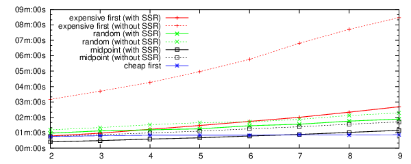
A naive controller works with the observable predicates $\{(heavy=true),(pos=0),(y<1)\}$, resets the clock $y$ each time a new box is arrived, and then move it to the next step (remove after the last iteration) each $2$ time units if the box is light and $5$ time units if the box is heavy. However, it is not necessary to use the expensive $(y<1)$ observable predicate, since a controller can move a box after each $3$ ($6$ for heavy box) time units, thus the time granularity of $3$ is enough and there is a controller that uses the observable predicates $\{(heavy=true),(pos=0),(y<3)\}$. Our implementation detects such an optimal solution, and Fig. 5 demonstrates an average time needed to compute this solution for different numbers of box processing steps $n$. You can see that the state space reusage heuristics improves the performance of the algorithm.

The game size for this model ranges from $4$ knowledge game states and $51$ symbolic NTA states when there are $2$ processing steps and only safety predicate is observable to $6417$ knowledge game states and $15554$ symbolic NTA states for $9$ processing steps and when all the available predicate are observable.

References

- [1] Israa AlAttili, Fred Houben, Georgeta Igna, Steffen Michels, Feng Zhu, and Frits W. Vaandrager. Adaptive scheduling of data paths using uppaal tiga. In QFM, pages 1–11, 2009.
- [2] Rajeev Alur and David L. Dill. A theory of timed automata. Theoretical Computer Science, 126:183–235, 1994.
- [3] Gerd Behrmann, Agnes Cougnard, Alexandre David, Emmanuel Fleury, Kim G. Larsen, and Didier Lime. Uppaal-tiga: Time for playing games! In Proceedings of the 19th International Conference on Computer Aided Verification, number 4590 in LNCS, pages 121–125. Springer, 2007.
- [4] Patricia Bouyer, Thomas Brihaye, Véronique Bruyère, and Jean-François Raskin. On the optimal reachability problem of weighted timed automata. Formal Methods in System Design, 31(2):135–175, 2007.
- [5] Patricia Bouyer, Franck Cassez, Emmanuel Fleury, and Kim Guldstrand Larsen. Optimal strategies in priced timed game automata. In FSTTCS, pages 148–160, 2004.
- [6] Patricia Bouyer, Deepak D’Souza, P. Madhusudan, and Antoine Petit. Timed control with partial observability. In CAV, volume 2725 of Lecture Notes in Computer Science, pages 180–192. Springer, 2003.
- [7] Thomas Brihaye, Véronique Bruyère, and Jean-François Raskin. On optimal timed strategies. In FORMATS, volume 3829 of Lecture Notes in Computer Science, pages 49–64. Springer, 2005.
- [8] F. Cassez, A. David, K. G. Larsen, D. Lime, and J.-F. Raskin. Timed control with observation based and stuttering invariant strategies. In Proceedings of the 5th International Symposium on Automated Technology for Verification and Analysis, volume 4762 of LNCS, pages 192–206. Springer, 2007.
- [9] Franck Cassez, Alexandre David, Emmanuel Fleury, Kim G. Larsen, and Didier Lime. Efficient on-the-fly algorithms for the analysis of timed games. In CONCUR’05, volume 3653 of LNCS, pages 66–80. Springer–Verlag, August 2005.
- [10] Franck Cassez, Thomas A. Henzinger, and Jean-François Raskin. A comparison of control problems for timed and hybrid systems. In Proc. 5th International Workshop on Hybrid Systems: Computation and Control (HSCC’02), volume 2289 of Lecture Notes in Computer Science, pages 134–148. Springer, 2002.
- [11] Franck Cassez, Jan J. Jessen, Kim G. Larsen, Jean-François Raskin, and Pierre-Alain Reynier. Automatic synthesis of robust and optimal controllers — an industrial case study. In Proceedings of the 12th International Conference on Hybrid Systems: Computation and Control, HSCC ’09, pages 90–104, Berlin, Heidelberg, 2009. Springer-Verlag.
- [12] A. Cesta, A. Finzi, S. Fratini, A. Orlandini, and E. Tronci. Flexible timeline-based plan verification. In Bärbel Mertsching, Marcus Hund, and Zaheer Aziz, editors, KI 2009: Advances in Artificial Intelligence, volume 5803 of Lecture Notes in Computer Science, pages 49–56. Springer Berlin / Heidelberg, 2009.
- [13] Krishnendu Chatterjee, Thomas A. Henzinger, Barbara Jobstmann, and Rohit Singh 0002. Quasy: Quantitative synthesis tool. In Parosh Aziz Abdulla and K. Rustan M. Leino, editors, TACAS, volume 6605 of Lecture Notes in Computer Science, pages 267–271. Springer, 2011.
- [14] Krishnendu Chatterjee, Rupak Majumdar, and Thomas A. Henzinger. Controller synthesis with budget constraints. In HSCC, volume 4981 of Lecture Notes in Computer Science, pages 72–86. Springer, 2008.
- [15] Rayna Dimitrova and Bernd Finkbeiner. Abstraction refinement for games with incomplete information. In FSTTCS, volume 2 of LIPIcs, pages 175–186. Schloss Dagstuhl - Leibniz-Zentrum fuer Informatik, 2008.
- [16] Thomas A. Henzinger, Ranjit Jhala, and Rupak Majumdar. Counterexample-guided control. In ICALP, volume 2719 of Lecture Notes in Computer Science, pages 886–902. Springer, 2003.
- [17] Rupak Majumdar and Paulo Tabuada, editors. Hybrid Systems: Computation and Control, 12th International Conference, HSCC 2009, San Francisco, CA, USA, April 13-15, 2009. Proceedings, volume 5469 of Lecture Notes in Computer Science. Springer, 2009.
- [18] Oded Maler, Amir Pnueli, and Joseph Sifakis. On the synthesis of discrete controllers for timed systems. In in E.W. Mayr and C. Puech (Eds), Proc. STACS’95, LNCS 900, pages 229–242. Springer, 1995.
- [19] Oded Maler, Amir Pnueli, and Joseph Sifakis. On the synthesis of discrete controllers for timed systems (an extended abstract). In STACS, pages 229–242, 1995.
- [20] Janusz Malinowski, Peter Niebert, and Pierre-Alain Reynier. A hierarchical approach for the synthesis of stabilizing controllers for hybrid systems. In Proc. 9th International Symposium on Automated Technology for Verification and Analysis (ATVA’11), volume 6996 of Lecture Notes in Computer Science, pages 198–212. Springer, 2011.
- [21] Andrea Orlandini, Alberto Finzi, Amedeo Cesta, and Simone Fratini. TGA-based controllers for flexible plan execution. In Joscha Bach and Stefan Edelkamp, editors, KI 2011: Advances in Artificial Intelligence, volume 7006 of Lecture Notes in Computer Science, pages 233–245. Springer Berlin / Heidelberg, 2011.
- [22] Jean-François Raskin, Krishnendu Chatterjee, Laurent Doyen, and Thomas A. Henzinger. Algorithms for omega-regular games with imperfect information. Logical Methods in Computer Science, 3(3), 2007.
- [23] John H. Reif. The complexity of two-player games of incomplete information. Journal of Computer and System Sciences, 29(2):274–301, October 1984.
- [24] Uri Zwick and Mike Paterson. The complexity of mean payoff games on graphs. Theoretical Computer Science, 158:343–359, 1996.
Appendix 0.A Proof of the theorem 4.1
Theorem 0.A.1
Consider a TGA with clocks , and an (infinite) set of available predicates and the safety objective . Determining whether there exists a finite set of predicates such that Player I wins in IISTG is undecidable.
Proof
The proof below adopts the construction of the proof of the undecidability of the existence of a sampling rate allowing controllability of a timed automata w.r.t. a safety objective, proved in [10].
The proof is by reduction to boundedness of -counter machines. It is based on the encoding of such a machine into a timed automaton described in [10]. We do not recall this construction here. Formally, we write , and recall that the construction involves a location over. The main property of this construction used in this proof is the following: given a rational number and denoting , the counters of never exceed value if and only if location over is not reachable in the semantics of sampled by . In addition, we slightly modify the construction as follows: we add a fresh clock which, along every transition, is systematically reset and checked to be positive. Note that this has no effect on the sampled semantics of the automaton, whatever the value of the sampling. We also consider that every transition are controllable.
We consider as the safety objective the set . The set of observable predicates is defined as , where is the set of predicates , for every location , and is the set of predicates , where . We will show that there exists a finite set of predicates for which the system is controllable if and only if the -counter machine is bounded.
Assume the machine is bounded, say by value . Thanks to the property of recalled above, the semantics of for the sampling rate never enters location over, and thus verifies the safety objective. We prove that the system is controllable for the (finite) set of predicates . The strategy of the controller is as follows: it alternates between delays (action skip) and discrete actions. As clock is reset on every transition, this allows to simulate a sampled behavior, for sampling rate . Indeed, after each discrete step, the value of clock is zero, and thus the predicate will become false exactly after time units. At this time, the controller proposes an action which is enabled. The outcome of this strategy is a run of under the sampled semantics, for the sampling rate . In particular, this run never enters location .
Conversely, we proceed by contradiction and assume that the machine is not bounded and that there exists a finite subset of which allows to control the system. Let us denote by the least common multiple of integers such that the predicate belongs to . Since we have modified the machine by requesting some positive delay to elapse between two discrete actions, and by the semantics of stuttering invariant strategies, we know that all the actions of the controller will be played on ticks of sampling (but not necessarily all of them, the controller could propose to wait, or could use a predicate which is a multiple of ). As a consequence, the controlled behavior of will be a subset of the sampling semantics of w.r.t. sampling unit . This constitutes a contradiction since, as the machine is not bounded and by properties of the construction of , any sampled behavior of will eventually either be blocked or reach location over. ∎
Appendix 0.B Proof of the theorem 5.1
Theorem 0.B.1
Let be a non-redundant sequence of solutions for some set and cost function .
Consider that the value of can be computed in polynomial time.
Then the problem of determining whether there exists a one-element extension
of that is still non-redundant for and is NP-complete.
First, we show that the problem is in NP. Indeed, a proof certificate is a sequence itself, and its fitness can be checked in polynomial time.
Next, we demonstrate the NP-hardness by showing the reduction from the vertex cover problem. Formally, a vertex cover of a graph is a set of vertices such that each edge of is incident to at least one vertex in . The vertex cover decision problem is to determine for a given and , whether there exists a vertex cover of the graph , and the size of the set should be at most . This problem is known to be NP-complete.
Consider, that we are given a graph and a constant , and we want to check if there exists a vertex cover of size at most . Consider also that , , and . Let’s choose the set to be equal to , where is a special element. Let’s define the value of the cost function to be equal to if and to be equal to , otherwise. Consider a set of subsets of , where , and contains all the vertices from that are not incident to the edge . Let’s order the elements from in a sequence such that for any . All the sets of this sequence are pairwise different (i.e. for ), and thus for any .
Let us consider a sequence
First, it can be easily seen that this sequence is non-redundant for the chosen and (since for any ).
And second, the sequence can be extended by one element such that the resulting sequence is still non-redundant iff there exists a vertex cover of size at most for the graph . Indeed, such an extension exists iff there exists a set such, that , and for all . Note that is monotonic and therefore implies that , and thus . Therefore, we should have (since ) and for any there should be some vertex that belongs to and doesn’t belong to . The latter is equivalent to the fact that there exists a set of vertices of size at most and any edge from is incident to at least one vertex in . This proves the NP-hardness. ∎
Appendix 0.C Proof of the theorem 5.2
Theorem 0.C.2
Suppose that , is the knowledge game for , is the knowledge game for and is the knowledge game for . Then the relation between the states of and is a bisimulation.
Suppose, that and .
First, we have and and thus .
Consider an action and a pair of bisimilar states and (i.e. ). It’s easy to see, that . Now we will demonstrate, that for any -successor of there is a bisimular -successor of and vice versa. More precisely, we will show that for any game states and , if and there are transitions and , then and thus .
Suppose, that and are equal to , and and are equal to .
First, it is easy to see that an LTS state belongs to the game state iff there exists a sequence of transitions , where , and for any . We call such a sequence a proof sequence for in .
Again, it’s easy to see, that an LTS state belongs to the set iff there exists a sequence of game transitions such that , , and for any we have . The latter is true iff there exists a sequence of transitions
such that and for any , we have and . We call such a sequence a proof sequence for in .
Now it’s easy to see, that the sets and coincide, since any proof sequence for in is a proof sequence for in . At the same time, any proof sequence for in is a proof sequence for in , if we compute the values of sequentially based on the changes of the function. More formally, we choose to be the largest integer such that for and any , .
This shows that and proves that is a bisimulation. ∎
Corollary 1
Player I wins in iff Player I wins in
According to the theorem 5.2 there is a bisimulation relation between and .
It’s easy to see that the bisimulation relation preserves the satisfiability of and formulas, i.e. for any pair of states , iff . Therefore Player I wins in iff Player I wins in .