Averages of -hadron, -hadron, and -lepton properties as of early 2012 Heavy Flavor Averaging Group (HFAG):
Abstract
This article reports world averages of measurements of -hadron, -hadron, and -lepton properties obtained by the Heavy Flavor Averaging Group (HFAG) using results available through the end of 2011. In some cases results available in the early part of 2012 are included. For the averaging, common input parameters used in the various analyses are adjusted (rescaled) to common values, and known correlations are taken into account. The averages include branching fractions, lifetimes, neutral meson mixing parameters, violation parameters, parameters of semileptonic decays and CKM matrix elements.
1 Introduction
Flavor dynamics is an important element in understanding the nature of particle physics. The accurate knowledge of properties of heavy flavor hadrons, especially hadrons, plays an essential role for determining the elements of the Cabibbo-Kobayashi-Maskawa (CKM) weak-mixing matrix [1, 2]. The operation of the Belle and BABAR factory experiments led to a large increase in the size of available meson, hadron and lepton samples, enabling dramatic improvement in the accuracies of related measurements. The CDF and D0 experiments at the Fermilab Tevatron have also provided important results in heavy flavor physics, most notably in the sector. The CERN Large Hadron Collider is now delivering high luminosity, enabling the collection of even higher statistics samples of and hadrons at the ATLAS, CMS, and (especially) LHCb experiments.
The Heavy Flavor Averaging Group (HFAG) was formed in 2002 to continue the activities of the LEP Heavy Flavor Steering group [3, *Abbaneo:2001bv_mod_cont]. This group was responsible for calculating averages of measurements of -flavor related quantities. HFAG has evolved since its inception and currently consists of seven subgroups:
- •
the “ Lifetime and Oscillations” subgroup provides averages for -hadron lifetimes, -hadron fractions in decay and collisions, and various parameters governing - and - mixing;
- •
the “Unitarity Triangle Parameters” subgroup provides averages for time-dependent asymmetry parameters and resulting determinations of the angles of the CKM unitarity triangle;
- •
the “Semileptonic Decays” subgroup provides averages for inclusive and exclusive -decay branching fractions, and subsequent determinations of the CKM matrix elements and ;
- •
the “ to Charm Decays” subgroup provides averages of branching fractions for decays to final states involving open charm or charmonium mesons;
- •
the “Rare Decays” subgroup provides averages of branching fractions and asymmetries for charmless, radiative, leptonic, and baryonic meson decays;
- •
the “Charm Physics” subgroup provides averages of branching fractions for meson hadronic and semileptonic decays, averages of - mixing and and violation parameters, and an average value for the decay constant . The subgroup also documents properties of charm baryons, and upper limits for rare and forbidden , , and decays.
- •
the “Tau Physics” subgroup provides documentation and averages for the lepton branching fractions and the resulting determination of the CKM matrix element , and documents upper limits for lepton-flavor-violating decays.
The “Lifetime and Oscillations” and “Semileptonic” subgroups were formed from the merger of four LEP working groups. The “Unitary Triangle,” “ to Charm Decays,” and “Rare Decays” subgroups were formed to provide averages for new results obtained from the factory experiments (and now also from the Fermilab Tevatron and CERN LHC experiments). The “Charm” and “Tau” subgroups were formed more recently in response to the wealth of new data concerning and decays. Subgroup typically include representatives from Belle and BABAR and, when relevant, CLEO, CDF, D0 and LHCb.
This article is an update of the last HFAG preprint, which used results available at least through the end of 2009 [5]. Here we report world averages using results available at least through the end of 2011. In some cases results available in the early part of 2012 have been included.11 1 The precise cut-off date for including results in the averages varies between subgroups. In general, we use all publicly available results that have written documentation. These include preliminary results presented at conferences or workshops. However, we do not use preliminary results that remain unpublished for an extended period of time, or for which no publication is planned. Close contacts have been established between representatives from the experiments and members of subgroups that perform averaging to ensure that the data are prepared in a form suitable for combinations.
In the case of obtaining a world average for which , where is the number of degrees of freedom in the average calculation, we do not scale the resulting error, as is presently done by the Particle Data Group [6]. Rather, we examine the systematics of each measurement to better understand them. Unless we find possible systematic discrepancies between the measurements, we do not apply any additional correction to the calculated error. We provide the confidence level of the fit as an indicator for the consistency of the measurements included in the average. In case some special treatment was necessary to calculate an average, or if an approximation used in an average calculation might not be sufficiently accurate (e.g., assuming Gaussian errors when the likelihood function indicates non-Gaussian behavior), we include a warning message.
Chapter 2 describes the methodology used for calculating averages. In the averaging procedure, common input parameters used in the various analyses are adjusted (rescaled) to common values, and, where possible, known correlations are taken into account. Chapters 3–9 present world average values from each of the subgroups listed above. A brief summary of the averages presented is given in Chapter 10. A complete listing of the averages and plots, including updates since this document was prepared, are also available on the HFAG web site:
2 Methodology
The general averaging problem that HFAG faces is to combine information provided by different measurements of the same parameter to obtain our best estimate of the parameter’s value and uncertainty. The methodology described here focuses on the problems of combining measurements performed with different systematic assumptions and with potentially-correlated systematic uncertainties. Our methodology relies on the close involvement of the people performing the measurements in the averaging process.
Consider two hypothetical measurements of a parameter , which might be summarized as
where the are statistical uncertainties, and the are contributions to the systematic uncertainty. One popular approach is to combine statistical and systematic uncertainties in quadrature
and then perform a weighted average of and , using their combined uncertainties, as if they were independent. This approach suffers from two potential problems that we attempt to address. First, the values of the may have been obtained using different systematic assumptions. For example, different values of the lifetime may have been assumed in separate measurements of the oscillation frequency . The second potential problem is that some contributions of the systematic uncertainty may be correlated between experiments. For example, separate measurements of may both depend on an assumed Monte-Carlo branching fraction used to model a common background.
The problems mentioned above are related since, ideally, any quantity that depends on has a corresponding contribution to the systematic error which reflects the uncertainty on itself. We assume that this is the case and use the values of and assumed by each measurement explicitly in our averaging (we refer to these values as and below). Furthermore, since we do not lump all the systematics together, we require that each measurement used in an average have a consistent definition of the various contributions to the systematic uncertainty. Different analyses often use different decompositions of their systematic uncertainties, so achieving consistent definitions for any potentially correlated contributions requires close coordination between HFAG and the experiments. In some cases, a group of systematic uncertainties must be combined to obtain a coarser description that is consistent between measurements. Systematic uncertainties that are uncorrelated with any other sources of uncertainty appearing in an average are lumped together with the statistical error, so that the only systematic uncertainties treated explicitly are those that are correlated with at least one other measurement via a consistently-defined external parameter . When asymmetric statistical or systematic uncertainties are quoted, we symmetrize them since our combination method implicitly assumes parabolic likelihoods for each measurement.
The fact that a measurement of is sensitive to the value of indicates that, in principle, the data used to measure could equally-well be used for a simultaneous measurement of and , as illustrated by the large contour in Fig. 1(a) for a hypothetical measurement. However, we often have an external constraint on the value of (represented by the horizontal band in Fig. 1(a)) that is more precise than the constraint from our data alone. Ideally, in such cases we would perform a simultaneous fit to and , including the external constraint, obtaining the filled contour and corresponding dashed one-dimensional estimate of shown in Fig. 1(a). Throughout, we assume that the external constraint on is Gaussian.

In practice, the added technical complexity of a constrained fit with extra free parameters is not justified by the small increase in sensitivity, as long as the external constraints are sufficiently precise when compared with the sensitivities to each of the data alone. Instead, the usual procedure adopted by the experiments is to perform a baseline fit with all fixed to nominal values , obtaining . This baseline fit neglects the uncertainty due to , but this error can be mostly recovered by repeating the fit separately for each external parameter with its value fixed at to obtain , as illustrated in Fig. 1(b). The absolute shift, , in the central value of is what the experiments usually quote as their systematic uncertainty on due to the unknown value of . Our procedure requires that we know not only the magnitude of this shift but also its sign. In the limit that the unconstrained data is represented by a parabolic likelihood, the signed shift is given by
| (1) |
where and are the statistical uncertainty on and the correlation between and in the unconstrained data. While our procedure is not equivalent to the constrained fit with extra parameters, it yields (in the limit of a parabolic unconstrained likelihood) a central value that agrees to and an uncertainty that agrees to .
In order to combine two or more measurements that share systematics due to the same external parameters , we would ideally perform a constrained simultaneous fit of all data samples to obtain values of and each , being careful to only apply the constraint on each once. This is not practical since we generally do not have sufficient information to reconstruct the unconstrained likelihoods corresponding to each measurement. Instead, we perform the two-step approximate procedure described below.
Figs. 2(a,b) illustrate two statistically-independent measurements, and , of the same hypothetical quantity (for simplicity, we only show the contribution of a single correlated systematic due to an external parameter ). As our knowledge of the external parameters evolves, it is natural that the different measurements of will assume different nominal values and ranges for each . The first step of our procedure is to adjust the values of each measurement to reflect the current best knowledge of the values and ranges of the external parameters , as illustrated in Figs. 2(c,b). We adjust the central values and correlated systematic uncertainties linearly for each measurement (indexed by ) and each external parameter (indexed by ):
| (2) | ||||
| (3) |
This procedure is exact in the limit that the unconstrained likelihoods of each measurement is parabolic.

The second step of our procedure is to combine the adjusted measurements, using the chi-square
| (4) |
and then minimize this to obtain the best values of and and their uncertainties, as illustrated in Fig. 3. Although this method determines new values for the , we do not report them since the reported by each experiment are generally not intended for this purpose (for example, they may represent a conservative upper limit rather than a true reflection of a 68% confidence level).

For comparison, the exact method we would perform if we had the unconstrained likelihoods available for each measurement is to minimize the simultaneous constrained likelihood
| (5) |
with an independent Gaussian external constraint on each
| (6) |
The results of this exact method are illustrated by the filled ellipses in Figs. 3(a,b) and agree with our method in the limit that each is parabolic and that each . In the case of a non-parabolic unconstrained likelihood, experiments would have to provide a description of itself to allow an improved combination. In the case of , experiments are advised to perform a simultaneous measurement of both and so that their data will improve the world knowledge about .
The algorithm described above is used as a default in the averages reported in the following sections. For some cases, somewhat simplified or more complex algorithms are used and noted in the corresponding sections. Some examples for extensions of the standard method for extracting averages are given here. These include the case where measurement errors depend on the measured value, i.e. are relative errors, unknown correlation coefficients and the breakdown of error sources.
For measurements with Gaussian errors, the usual estimator for the average of a set of measurements is obtained by minimizing the following :
| (7) |
where is the measured value for input and is the variance of the distribution from which was drawn. The value of at minimum is our estimator for the average. (This discussion is given for independent measurements for the sake of simplicity; the generalization to correlated measurements is straightforward, and has been used when averaging results.) The true are unknown but typically the error as assigned by the experiment is used as an estimator for it. Caution is advised, however, in the case where depends on the value measured for . Examples of this include an uncertainty in any multiplicative factor (like an acceptance) that enters the determination of , i.e. the dependence of Poisson statistics, where and . Failing to account for this type of dependence when averaging leads to a biased average. Biases in the average can be avoided (or at least reduced) by minimizing the following :
| (8) |
In the above is the uncertainty assigned to input that includes the assumed dependence of the stated error on the value measured. As an example, consider a pure acceptance error, for which . It is easily verified that solving Eq. 8 leads to the correct behavior, namely
i.e. weighting by the inverse square of the fractional uncertainty, . It is sometimes difficult to assess the dependence of on from the errors quoted by experiments.
Another issue that needs careful treatment is the question of correlation among different measurements, e.g. due to using the same theory for calculating acceptances. A common practice is to set the correlation coefficient to unity to indicate full correlation. However, this is not a “conservative” thing to do, and can in fact lead to a significantly underestimated uncertainty on the average. In the absence of better information, the most conservative choice of correlation coefficient between two measurements and is the one that maximizes the uncertainty on due to that pair of measurements:
| (9) |
namely
| (10) |
which corresponds to setting . Setting when can lead to a significant underestimate of the uncertainty on , as can be seen from Eq. 9.
Finally, we carefully consider the various sources of error contributing to the overall uncertainty of an average. The overall covariance matrix is constructed from a number of individual sources, e.g. . The variance on the average can be written
| (11) |
Written in this form, one can readily determine the contribution of each source of uncertainty to the overall uncertainty on the average. This breakdown of the uncertainties is used in the following sections.
Following the prescription described above, the central values and errors are rescaled to a common set of input parameters in the averaging procedures according to the dependency on any of these input parameters. We try to use the most up-to-date values for these common inputs and the same values among the HFAG subgroups. For the parameters whose averages are produced by HFAG, we use the values in the current update cycle. For other external parameters, we use the most recent PDG values available (usually Ref. [6]). The parameters and values used are listed in each subgroup section.
3 -hadron production fractions, lifetimes and mixing parameters
Quantities such as -hadron production fractions, -hadron lifetimes, and neutral -meson oscillation frequencies have been studied in the nineties at LEP and SLC ( colliders at ) as well as at the first version of the Tevatron ( collider at ). Since then precise measurements of the and mesons have also been performed at the asymmetric factories, KEKB and PEPII ( colliders at ) while measurements related to the other -hadrons, in particular , and , have been performed at the upgraded Tevatron () and are continuing at the LHC ( collider at ). In most cases, these basic quantities, although interesting by themselves, became necessary ingredients for the more complicated and refined analyses at the asymmetric factories, the Tevatron and the LHC, in particular the time-dependent asymmetry measurements. It is therefore important that the best experimental values of these quantities continue to be kept up-to-date and improved.
In several cases, the averages presented in this chapter are needed and used as input for the results given in the subsequent chapters. Within this chapter, some averages need the knowledge of other averages in a circular way. This coupling, which appears through the -hadron fractions whenever inclusive or semi-exclusive measurements have to be considered, has reduced drastically in the past several years with increasingly precise exclusive measurements becoming available and dominating practically all averages.
In addition to -hadron fractions, lifetimes and mixing parameters, this chapter also deals with the -violating phase , which is the phase difference between the mixing amplitude and the decay amplitude. The angle , which is the equivalent of for the system, is discussed in Chapter 4.
3.1 -hadron production fractions
We consider here the relative fractions of the different -hadron species found in an unbiased sample of weakly-decaying hadrons produced under some specific conditions. The knowledge of these fractions is useful to characterize the signal composition in inclusive -hadron analyses, to predict the background composition in exclusive analyses, or to convert (relative) observe rates into (relative) branching fraction measurements. Many -physics analyses need these fractions as input. We distinguish here the following three conditions: decays, decays, and high-energy collisions (including decays).
3.1.1 -hadron production fractions in decays
Only pairs of the two lightest (charged and neutral) mesons can be produced in decays, and it is enough to determine the following branching fractions:
| (12) | |||||
| (13) |
In practice, most analyses measure their ratio
| (14) |
which is easier to access experimentally. Since an inclusive (but separate) reconstruction of and is difficult, specific exclusive decay modes, and , are usually considered to perform a measurement of , whenever they can be related by isospin symmetry (for example and ). Under the assumption that , i.e. that isospin invariance holds in these decays, the ratio of the number of reconstructed and mesons is proportional to
| (15) |
where and are the and lifetimes respectively. Hence the primary quantity measured in these analyses is , and the extraction of with this method therefore requires the knowledge of the lifetime ratio.
| Experiment | Ref. | Decay modes | Published value of | Assumed value |
| and year | or method | of | ||
| CLEO, 2001 | [10] | |||
| BABAR, 2002 | [8] | |||
| CLEO, 2002 | [11] | |||
| Belle, 2003 | [12] | dilepton events | ||
| BABAR, 2004 | [9] | |||
| BABAR, 2005 | [7] | |||
| Average | (tot) |
The published measurements of are listed in Table 1 together with the corresponding assumed values of . All measurements are based on the above-mentioned method, except the one from Belle, which is a by-product of the mixing frequency analysis using dilepton events (but note that it also assumes isospin invariance, namely ). The latter is therefore treated in a slightly different manner in the following procedure used to combine these measurements:
- •
each published value of from CLEO and BABAR is first converted back to the original measurement of , using the value of the lifetime ratio assumed in the corresponding analysis;
- •
a simple weighted average of these original measurements of from CLEO and BABAR (which do not depend on the assumed value of the lifetime ratio) is then computed, assuming no statistical or systematic correlations between them;
- •
the weighted average of is converted into a value of , using the latest average of the lifetime ratios, (see Sec. 3.2.3);
- •
the Belle measurement of is adjusted to the current values of and (see Sec. 3.2.3), using the quoted systematic uncertainties due to these parameters;
- •
the combined value of from CLEO and BABAR is averaged with the adjusted value of from Belle, assuming a 100% correlation of the systematic uncertainty due to the limited knowledge on ; no other correlation is considered.
The resulting global average,
| (16) |
is consistent with an equal production of charged and neutral mesons, although only at the level.
On the other hand, the BABAR collaboration has performed a direct measurement of the fraction using an original method, which does not rely on isospin symmetry nor requires the knowledge of . Its analysis, based on a comparison between the number of events where a single decay could be reconstructed and the number of events where two such decays could be reconstructed, yields [13]
| (17) |
The two results of Eqs. (16) and (17) are of very different natures and completely independent of each other. Their product is equal to , while another combination of them gives , compatible with unity. Assuming22 2 A few non- decay modes of the (, , ) have been observed with branching fractions of the order of [14, *Sokolov:2006sd, *Aubert_mod:2008bv], corresponding to a partial width several times larger than that in the channel. However, this can still be neglected and the assumption remains valid in the present context of the determination of and . , also consistent with CLEO’s observation that the fraction of decays to pairs is larger than 0.96 at 95% CL [17], the results of Eqs. (16) and (17) can be averaged (first converting Eq. (16) into a value of ) to yield the following more precise estimates:
| (18) |
The latter ratio differs from one by .
3.1.2 -hadron production fractions in decays
Hadronic events produced in collisions at the energy can be classified into three categories: light-quark (, , , ) continuum events, continuum events, and events. The latter two cannot be distinguished and will be called events in the following. These events, which also include events because of possible initial-state radiation, can hadronize in different final states. We define as the fraction of events with a pair of non-strange bottom mesons (, , , , , , , , and final states, where denotes a or meson and denotes a or meson), as the fraction of events with a pair of strange bottom mesons (, , , and final states), and as the fraction of events without bottom meson in the final state. Note that the excited bottom-meson states decay via and . These fractions satisfy
| (19) |
| Experiment, year, dataset | Decay mode or method | Value of |
| CLEO, 2006, 0.42 [19] | ||
| CLEO average of above 3 | ||
| Belle, 2006, 1.86 [20] | ||
| Belle average of above 2 | ||
| Belle, 2010, 23.6 [18] | ||
| Average of all above after adjustments to inputs of Table 3 | ||
| Branching fraction | Value | Explanation and reference |
|---|---|---|
| derived from [21] | ||
| model-dependent estimate [22] | ||
| [21] | ||
| derived from [21] | ||
| model-dependent estimate [20, 22] | ||
| [21] | ||
| world average [21, 19] | ||
| model-dependent estimate [19] |
The CLEO and Belle collaborations have published in 2006 measurements of several inclusive branching fractions, , and , from which they extracted the model-dependent estimates of reported in Table 2. This extraction was performed under the implicit assumption , using the relation
| (20) |
and similar relations for and . We list also in Table 2 the values of derived from measurements of [19, 18], as well as our average value of , all obtained under the assumption .
However, the assumption is no longer valid since the observation of decays to , , and [23], and more recently to and [24]. The sum of these measured branching fractions, adding also the contributions of the , , , , and final states assuming isospin conservation, amounts to
which is to be considered as a lower bound for . Following the method described in , we perform a fit of the original measurements of the branching fractions of Refs. [19, 20, 18], using the inputs of Table 3, the relations of Eqs. (19) and (20) and the one-sided Gaussian constraint , to simultaneously extract , and . Taking all known correlations into account, the best fit values are
| (21) | |||||
| (22) | |||||
| (23) |
where the strongly asymmetric uncertainty on is due to the one-sided constraint from the observed decays. These results, together with their correlation, imply
| (24) |
in fair agreement with the results of a BABAR analysis [26] performed as a function of centre-of-mass energy33 3 This has not been included in the average, since no numerical value is given for in ..
3.1.3 -hadron production fractions at high energy
At high energy, all species of weakly-decaying hadrons may be produced, either directly or in strong and electromagnetic decays of excited hadrons. It is often assumed that the fractions of these different species are the same in unbiased samples of high- jets originating from decays, from collisions at the Tevatron, or from collisions at the LHC. This hypothesis is plausible under the condition that the square of the momentum transfer to the produced quarks, , is large compared with the square of the hadronization energy scale, . On the other hand, there is no strong argument to claim that the fractions at different machines should be strictly equal, so this assumption should be checked experimentally. Although the available data is not sufficient at this time to perform a definitive check, it is expected that more refined analyses of the Tevatron Run II data and new analyses from LHC experiments may improve this situation and allow one to confirm or disprove this assumption with reasonable confidence. Meanwhile, the attitude adopted here is that these fractions are assumed to be equal at all high-energy colliders until demonstrated otherwise by experiment. However, both CDF and LHCb report a dependence for production relative to and ; the number of baryons observed at low is enhanced with respect to that seen at LEP at higher . Therefore we present three sets of complete averages: one set including only measurements performed at LEP, a second set including only measurements performed at the Tevatron, a third set including measurements performed at LEP, Tevatron and LHCb. The LHCb production fractions results, by themselves, are still incomplete, lacking measurements on the production of other weakly decaying heavy flavour baryons, and , and a measurement of giving an extra constraint between and .
Contrary to what happens in the charm sector where the fractions of and are different, the relative amount of and is not affected by the electromagnetic decays of excited and states and strong decays of excited and states. Decays of the type also contribute to the and rates, but with the same magnitude if mass effects can be neglected. We therefore assume equal production of and . We also neglect the production of weakly-decaying states made of several heavy quarks (like and other heavy baryons) which is known to be very small. Hence, for the purpose of determining the -hadron fractions, we use the constraints
| (25) |
where , , and are the unbiased fractions of , , and baryons, respectively.
The LEP experiments have measured [29, *Acton:1992zq, *Buskulic:1995bd], [32, 33] and [34, 35]44 4 The DELPHI result of is considered to supersede an older one [36]. from partially reconstructed final states including a lepton, from protons identified in events [37], and the production rate of charged hadrons [38]. Ratios of -hadron fractions have been measured at CDF using lepton+charm final states [39, 40, 41]55 5 CDF updated their measurement of / [39] to account for a measured dependence between exclusively reconstructed and [41]. and double semileptonic decays with and final states [42]. Measurements of the production of other heavy flavour baryons at the Tevatron are included in the determination of [43, 44, 45]66 6 D0 reports . We use the CDF+D0 average of to obtain and then combine with the CDF result. using the constraint
| (26) | |||||
where isospin invariance is assumed in the production of and . Other -baryons are expected to decay strongly or electromagnetically to those baryons listed. For the production measurements, both CDF and D0 reconstruct their -baryons exclusively to final states which include a and a hyperon (, and ). We assume that the partial decay width of a -baryon to a and the corresponding hyperon is equal to the partial width of any other -baryon to a and the corresponding hyperon. LHCb has also measured ratios of -hadron fractions, and , in lepton+charm final states [46] and in fully reconstructed hadronic final states using theoretical values for the branching fractions of two-body and decays [47].
Both CDF and LHCb observe a dependence in the relative fractions [41, 46]77 7 CDF compares the distribution of fully reconstructed with which compares up to a scale factor. LHCb compares the in the lepton+charm system between and and comparing .. No dependence is yet observed for . CDF chose to correct an older result to account for the dependence whereas LHCb chose to report a linear dependence of , which yields unphysical results for . In a second result, CDF binned their data in of the electron+charm system. Figure 4 shows the ratio as a function of this , as measured by both CDF and LHCb. Two fits are performed. The first fit using the LHCb parameterization yields . A second fit using a simple exponential yields . A common systematic uncertainty of 26% on the scale of both results arises from the branching fraction. The quality of the two fits are similar, but the second parameterization gives a physical result for all . A value of is also calculated for LEP and placed at the approximate for the lepton+charm system, but this value does not participate in any fit. Note that the dependence of combined with the constraint in Eq. (25) implies a compensating dependence in one or more of the production fractions, , , or .

In order to combine or compare LHCb results with other experiments, the -dependent is weighted by the spectrum88 8 In practice the LHCb data are given in 14 bins in and with a full covariance matrix [46]. The weighted average is calculated as , where , is a vector of measurements, is the inverse covariance matrix and is the transpose of the design matrix (vector of 1’s). Table 4 compares the -weighted LHCb data with comparable averages from the CDF. The average CDF and LHCb data are in good agreement despite the hadrons being produced in different kinematic regimes.
| Quantity | CDF | LHCb |
|---|---|---|
| Average lepton+charm | GeV/ | GeV/ |
| Pseudo-rapidity range |
All these published results have been combined following the procedure and assumptions described in , to yield , and under the constraints of Eq. (25). Repeating the combinations, for LEP and the Tevatron, we obtain , and when using the LEP data only, , when using the Tevatron data only. As noted previously, the LHCb data are insufficient to determine a complete set of -hadron production fractions. The world averages (LEP, Tevatron and LHCb) for the various fractions are presented here for comparison with previous averages. Significant differences exist between the LEP and Tevatron fractions, therefore use of the world averages should be taken with some care. For these combinations other external inputs are used, e.g. the branching ratios of mesons to final states with a , or in semileptonic decays, which are needed to evaluate the fraction of semileptonic decays with a in the final state.
Time-integrated mixing analyses performed with lepton pairs from events produced at high-energy colliders measure the quantity
| (27) |
where and are the fractions of and hadrons in a sample of semileptonic -hadron decays, and where and are the and time-integrated mixing probabilities. Assuming that all hadrons have the same semileptonic decay width implies , where is the ratio of the lifetime of species to the average -hadron lifetime . Hence measurements of the mixing probabilities , and can be used to improve our knowledge of , , and . In practice, the above relations yield another determination of obtained from and mixing information,
| (28) |
where .
The published measurements of performed by the LEP experiments have been combined by the LEP Electroweak Working Group to yield [48]. This can be compared with the Tevatron average, , obtained from D0 [49] and CDF [50] measurements with Run II data.99 9 As explained in , a previous CDF analysis [51] performed with Run I data overlooked a background component, so the corresponding result is not included in the average. The two averages agree, showing no evidence that the production fractions of and mesons at the peak or at the Tevatron are different. We combine these two results in a simple weighted average, assuming no correlations, and obtain .
| Quantity | decays | Tevatron | LHCb [46] | all | |
|---|---|---|---|---|---|
| Mixing probability | |||||
| or fraction | |||||
| fraction | |||||
| -baryon fraction | |||||
| ratio | |||||
Introducing the average in Eq. (28), together with our world average (see Eq. (57) of Sec. 3.3.1), the assumption (justified by Eq. (66) in Sec. 3.3.2), the best knowledge of the lifetimes (see Sec. 3.2) and the estimate of given above, yields (or using only LEP data, or using only Tevatron data), an estimate dominated by the mixing information. Taking into account all known correlations (including the one introduced by ), this result is then combined with the set of fractions obtained from direct measurements (given above), to yield the improved estimates of Table 5, still under the constraints of Eq. (25). As can be seen, our knowledge on the mixing parameters substantially reduces the uncertainty on . It should be noted that the results are correlated, as indicated in Table 5.
3.2 -hadron lifetimes
In the spectator model the decay of -flavoured hadrons is governed entirely by the flavour changing transition (). For this very reason, lifetimes of all -flavoured hadrons are the same in the spectator approximation regardless of the (spectator) quark content of the . In the early 1990’s experiments became sophisticated enough to start seeing the differences of the lifetimes among various species. The first theoretical calculations of the spectator quark effects on lifetime emerged only few years earlier.
Currently, most of such calculations are performed in the framework of the Heavy Quark Expansion, HQE. In the HQE, under certain assumptions (most important of which is that of quark-hadron duality), the decay rate of an to an inclusive final state is expressed as the sum of a series of expectation values of operators of increasing dimension, multiplied by the correspondingly higher powers of :
| (29) |
where is the relevant combination of the CKM matrix elements. Coefficients of this expansion, known as Operator Product Expansion [52, *Chay:1990da, *Bigi:1992su, *Bigi:1992su_erratum], can be calculated perturbatively. Hence, the HQE predicts in the form of an expansion in both and . The precision of current experiments makes it mandatory to go to the next-to-leading order in QCD, i.e. to include correction of the order of to the ’s. All non-perturbative physics is shifted into the expectation values of operators . These can be calculated using lattice QCD or QCD sum rules, or can be related to other observables via the HQE [56, *Bellini:1996ra]. One may reasonably expect that powers of provide enough suppression that only the first few terms of the sum in Eq. (29) matter.
Theoretical predictions are usually made for the ratios of the lifetimes (with chosen as the common denominator) rather than for the individual lifetimes, for this allows several uncertainties to cancel. The precision of the current HQE calculations (see Refs. [58, *Beneke:2002rj, *Franco:2002fc, 61, *Gabbiani:2003pq, 63] for the latest updates) is in some instances already surpassed by the measurements, e.g. in the case of . Also, HQE calculations are not assumption-free. More accurate predictions are a matter of progress in the evaluation of the non-perturbative hadronic matrix elements and verifying the assumptions that the calculations are based upon. However, the HQE, even in its present shape, draws a number of important conclusions, which are in agreement with experimental observations:
- •
The heavier the mass of the heavy quark the smaller is the variation in the lifetimes among different hadrons containing this quark, which is to say that as we retrieve the spectator picture in which the lifetimes of all ’s are the same. This is well illustrated by the fact that lifetimes are rather similar in the sector, while they differ by large factors in the sector ().
- •
The non-perturbative corrections arise only at the order of , which translates into differences among lifetimes of only a few percent.
- •
It is only the difference between meson and baryon lifetimes that appears at the level. The splitting of the meson lifetimes occurs at the level, yet it is enhanced by a phase space factor with respect to the leading free decay.
To ensure that certain sources of systematic uncertainty cancel, lifetime analyses are sometimes designed to measure a ratio of lifetimes. However, because of the differences in decay topologies, abundance (or lack thereof) of decays of a certain kind, etc., measurements of the individual lifetimes are more common. In the following section we review the most common types of the lifetime measurements. This discussion is followed by the presentation of the averaging of the various lifetime measurements, each with a brief description of its particularities.
3.2.1 Lifetime measurements, uncertainties and correlations
In most cases lifetime of an is estimated from a flight distance and a factor which is used to convert the geometrical distance into the proper decay time. Methods of accessing lifetime information can roughly be divided in the following five categories:
- 1.
Inclusive (flavour-blind) measurements. These measurements are aimed at extracting the lifetime from a mixture of -hadron decays, without distinguishing the decaying species. Often the knowledge of the mixture composition is limited, which makes these measurements experiment-specific. Also, these measurements have to rely on Monte Carlo for estimating the factor, because the decaying hadrons are not fully reconstructed. On the bright side, these usually are the largest statistics -hadron lifetime measurements that are accessible to a given experiment, and can, therefore, serve as an important performance benchmark.
- 2.
Measurements in semileptonic decays of a specific . from produces pair () in about 21% of the cases. Electron or muon from such decays is usually a well-detected signature, which provides for clean and efficient trigger. quark from transition and the other quark(s) making up the decaying combine into a charm hadron, which is reconstructed in one or more exclusive decay channels. Knowing what this charmed hadron is allows one to separate, at least statistically, different species. The advantage of these measurements is in statistics, which usually is superior to that of the exclusively reconstructed decays. Some of the main disadvantages are related to the difficulty of estimating lepton+charm sample composition and Monte Carlo reliance for the factor estimate.
- 3.
Measurements in exclusively reconstructed hadronic decays. These have the advantage of complete reconstruction of decaying , which allows one to infer the decaying species as well as to perform precise measurement of the factor. Both lead to generally smaller systematic uncertainties than in the above two categories. The downsides are smaller branching ratios, larger combinatoric backgrounds, especially in and multi-body decays, or in a hadron collider environment with non-trivial underlying event. are relatively clean and easy to trigger on , but their branching fraction is only about 1%.
- 4.
Measurements at asymmetric B factories.
In the decay, the mesons ( or ) are essentially at rest in the frame. This makes direct lifetime measurements impossible in experiments at symmetric colliders producing at rest. At asymmetric factories the meson is boosted resulting in and moving nearly parallel to each other with the same boost. The lifetime is inferred from the distance separating the and decay vertices along the beam axis and from the boost known from the beam energies. This boost is equal to (0.43) in the BABAR (Belle) experiment, resulting in an average decay length of approximately 250 (190) m.
In order to determine the charge of the mesons in each event, one of the them is fully reconstructed in a semileptonic or hadronic decay mode. The other is typically not fully reconstructed, only the position of its decay vertex is determined from the remaining tracks in the event. These measurements benefit from large statistics, but suffer from poor proper time resolution, comparable to the lifetime itself. This resolution is dominated by the uncertainty on the decay vertices, which is typically 50 (100) m for a fully (partially) reconstructed meson. With very large future statistics, the resolution and purity could be improved (and hence the systematics reduced) by fully reconstructing both mesons in the event.
- 5.
Direct measurement of lifetime ratios. This method has so far been only applied in the measurement of . The ratio of the lifetimes is extracted from the dependence of the observed relative number of and candidates (both reconstructed in semileptonic decays) on the proper decay time.
In some of the latest analyses, measurements of two (e.g. and ) or three (e.g. , , and ) quantities are combined. This introduces correlations among measurements. Another source of correlations among the measurements are the systematic effects, which could be common to an experiment or to an analysis technique across the experiments. When calculating the averages, such correlations are taken into account per general procedure, described in .
3.2.2 Inclusive -hadron lifetimes
The inclusive hadron lifetime is defined as where are the individual species lifetimes and are the fractions of the various species present in an unbiased sample of weakly-decaying hadrons produced at a high-energy collider.1010 10 In principle such a quantity could be slightly different in decays and at the Tevatron, in case the fractions of -hadron species are not exactly the same; see the discussion in Sec. 3.1.3. This quantity is certainly less fundamental than the lifetimes of the individual species, the latter being much more useful in comparisons of the measurements with the theoretical predictions. Nonetheless, we perform the averaging of the inclusive lifetime measurements for completeness as well as for the reason that they might be of interest as “technical numbers.”
| Experiment | Method | Data set | (ps) | Ref. |
| ALEPH | Dipole | 91 | [65] | |
| DELPHI | All track i.p. (2D) | 91–92 | [66]a | |
| DELPHI | Sec. vtx | 91–93 | [67]a | |
| DELPHI | Sec. vtx | 94–95 | [68] | |
| L3 | Sec. vtx + i.p. | 91–94 | [69]b | |
| OPAL | Sec. vtx | 91–94 | [70] | |
| SLD | Sec. vtx | 93 | [71] | |
| Average set 1 ( vertex) | ||||
| ALEPH | Lepton i.p. (3D) | 91–93 | [72] | |
| L3 | Lepton i.p. (2D) | 91–94 | [69]b | |
| OPAL | Lepton i.p. (2D) | 90–91 | [73] | |
| Average set 2 () | ||||
| CDF1 | vtx | 92–95 | [74] | |
| ATLAS | vtx | 2010 | [75] | |
| Average set 3 () | ||||
| Average of all above | ||||
| a The combined DELPHI result quoted in [67] is 1.575 0.010 0.026 ps. | ||||
| b The combined L3 result quoted in [69] is 1.549 0.009 0.015 ps. | ||||
In practice, an unbiased measurement of the inclusive lifetime is difficult to achieve, because it would imply an efficiency which is guaranteed to be the same across species. So most of the measurements are biased. In an attempt to group analyses which are expected to select the same mixture of hadrons, the available results (given in Table 6) are divided into the following three sets:
- 1.
measurements at LEP and SLD that accept any -hadron decay, based on topological reconstruction (secondary vertex or track impact parameters);
- 2.
measurements at LEP based on the identification of a lepton from a decay; and
- 3.
measurements at the Tevatron based on inclusive reconstruction, where the is fully reconstructed.
The measurements of the first set are generally considered as estimates of , although the efficiency to reconstruct a secondary vertex most probably depends, in an analysis-specific way, on the number of tracks coming from the vertex, thereby depending on the type of the . Even though these efficiency variations can in principle be accounted for using Monte Carlo simulations (which inevitably contain assumptions on branching fractions), the mixture in that case can remain somewhat ill-defined and could be slightly different among analyses in this set.
On the contrary, the mixtures corresponding to the other two sets of measurements are better defined in the limit where the reconstruction and selection efficiency of a lepton or a from an does not depend on the decaying hadron type. These mixtures are given by the production fractions and the inclusive branching fractions for each species to give a lepton or a . In particular, under the assumption that all hadrons have the same semileptonic decay width, the analyses of the second set should measure which is necessarily larger than if lifetime differences exist. Given the present knowledge on and , is expected to be of the order of 0.01 .
Measurements by SLC and LEP experiments are subject to a number of common systematic uncertainties, such as those due to (lack of knowledge of) and fragmentation, and decay models, , , , , and decay multiplicity. In the averaging, these systematic uncertainties are assumed to be 100% correlated. The averages for the sets defined above (also given in Table 6) are
| (30) | |||||
| (31) | |||||
| (32) |
whereas an average of all measurements, ignoring mixture differences, yields .
3.2.3 and lifetimes and their ratio
| Experiment | Method | Data set | (ps) | Ref. |
| ALEPH | 91–95 | [76] | ||
| ALEPH | Exclusive | 91–94 | [77] | |
| ALEPH | Partial rec. | 91–94 | [77] | |
| DELPHI | 91–93 | [78] | ||
| DELPHI | Charge sec. vtx | 91–93 | [79] | |
| DELPHI | Inclusive | 91–93 | [80] | |
| DELPHI | Charge sec. vtx | 94–95 | [68] | |
| L3 | Charge sec. vtx | 94–95 | [81] | |
| OPAL | 91–93 | [82] | ||
| OPAL | Charge sec. vtx | 93–95 | [83] | |
| OPAL | Inclusive | 91–00 | [84] | |
| SLD | Charge sec. vtx | 93–95 | [85]a | |
| SLD | Charge sec. vtx | 93–95 | [85]a | |
| CDF1 | 92–95 | [86] | ||
| CDF1 | Excl. | 92–95 | [87] | |
| CDF2 | Excl. , | 02–09 | [88, *Abulencia:2006dr_mod_cont] | |
| D0 | Excl. | 03–07 | [90, *Abazov:2005sa_mod_cont] | |
| D0 | Excl. | 02–11 | [92, *Abazov:2007sf_mod_cont, *Abazov:2004bn_mod_cont] | |
| BABAR | Exclusive | 99–00 | [95] | |
| BABAR | Inclusive | 99–01 | [96, *Aubert:2002gi_erratum] | |
| BABAR | Exclusive | 99–02 | [98] | |
| BABAR | Incl. , | 99–01 | [99] | |
| BABAR | Inclusive | 99–04 | [100] | |
| Belle | Exclusive | 00–03 | [101] | |
| ATLAS | Excl. | 2010 | [102]p | |
| LHCb | Excl. | 2010 | [103]p | |
| LHCb | Excl. | 2010 | [103]p | |
| Average | ||||
| a The combined SLD result quoted in [85] is 1.64 0.08 0.08 ps. | ||||
| p Preliminary. | ||||
After a number of years of dominating these averages the LEP experiments yielded the scene to the asymmetric factories and the Tevatron experiments. The factories have been very successful in utilizing their potential – in only a few years of running, BABAR and, to a greater extent, Belle, have struck a balance between the statistical and the systematic uncertainties, with both being close to (or even better than) the impressive 1%. In the meanwhile, CDF and D0 have emerged as significant contributors to the field as the Tevatron Run II data flowed in, with CDF eventually providing the most precise results.
| Experiment | Method | Data set | (ps) | Ref. |
| ALEPH | 91–95 | [76] | ||
| ALEPH | Exclusive | 91–94 | [77] | |
| DELPHI | 91–93 | [78]a | ||
| DELPHI | Charge sec. vtx | 91–93 | [79]a | |
| DELPHI | Charge sec. vtx | 94–95 | [68] | |
| L3 | Charge sec. vtx | 94–95 | [81] | |
| OPAL | 91–93 | [82] | ||
| OPAL | Charge sec. vtx | 93–95 | [83] | |
| SLD | Charge sec. vtx | 93–95 | [85]b | |
| SLD | Charge sec. vtx | 93–95 | [85]b | |
| CDF1 | 92–95 | [86] | ||
| CDF1 | Excl. | 92–95 | [87] | |
| CDF2 | Excl. | 02–09 | [88, *Abulencia:2006dr_mod_cont] | |
| CDF2 | Excl. | 02–06 | [104] | |
| BABAR | Exclusive | 99–00 | [95] | |
| Belle | Exclusive | 00–03 | [101] | |
| LHCb | Excl. | 2010 | [103]p | |
| Average | ||||
| a The combined DELPHI result quoted in [79] is ps. | ||||
| b The combined SLD result quoted in [85] is ps. | ||||
| p Preliminary. | ||||
At present time we are in an interesting position of having three sets of measurements (from LEP/SLC, factories and the Tevatron) that originate from different environments, obtained using substantially different techniques and are precise enough for incisive comparison.
| Experiment | Method | Data set | Ratio | Ref. |
| ALEPH | 91–95 | [76] | ||
| ALEPH | Exclusive | 91–94 | [77] | |
| DELPHI | 91–93 | [78] | ||
| DELPHI | Charge sec. vtx | 91–93 | [79] | |
| DELPHI | Charge sec. vtx | 94–95 | [68] | |
| L3 | Charge sec. vtx | 94–95 | [81] | |
| OPAL | 91–93 | [82] | ||
| OPAL | Charge sec. vtx | 93–95 | [83] | |
| SLD | Charge sec. vtx | 93–95 | [85]a | |
| SLD | Charge sec. vtx | 93–95 | [85]a | |
| CDF1 | 92–95 | [86] | ||
| CDF1 | Excl. | 92–95 | [87] | |
| CDF2 | Excl. | 02–09 | [88, *Abulencia:2006dr_mod_cont] | |
| D0 | ratio | 02–04 | [105] | |
| BABAR | Exclusive | 99–00 | [95] | |
| Belle | Exclusive | 00–03 | [101] | |
| Average | ||||
| a The combined SLD result quoted in [85] is . | ||||
The averaging of , and measurements is summarized1111 11 We do not include the old unpublished measurements of Refs. [106, 107]. in Tables 7, 8, and 9. For we averaged only the measurements of this quantity provided by experiments rather than using all available knowledge, which would have included, for example, and measurements which did not contribute to any of the ratio measurements.
The following sources of correlated (within experiment/machine) systematic uncertainties have been considered:
- •
- •
for BABAR measurements – alignment, scale, PEP-II boost, sample composition (where applicable);
- •
for D0 and CDF Run II measurements – alignment (separately within each experiment).
The resultant averages are:
| (33) | |||||
| (34) | |||||
| (35) |
3.2.4 lifetimes
Like neutral kaons, neutral mesons contain short- and long-lived components, since the light (L) and heavy (H) eigenstates, and , differ not only in their masses, but also in their total decay widths, with a decay width difference defined as . Neglecting violation in mixing, which is expected to be very small [108, *Lenz:2006hd, 110], the mass eigenstates are also eigenstates, with the light state being -even and the heavy state being -odd. While the decay width difference can be neglected in the system, the system exhibits a significant value of : the sign of is known to be positive [111], i.e. the heavy eigenstates lives longer than the light eigenstate. Specific measurements of and are explained and averaged in Sec. 3.3.2, but the results for , and the mean lifetime, defined as , are also quoted at the end of this section.
Many lifetime analyses, in particular the early ones performed before the non-zero value of was firmly established, ignore and fit the proper time distribution of a sample of candidates reconstructed in a certain final state with a model assuming a single exponential function for the signal. We denote such effective lifetime measurements as ; their true values may lie a priori anywhere between and , depending on the proportion of and in the final state . Table 10 summarizes the effective lifetime measurements.
Averaging measurements of over several final states will yield a result corresponding to an ill-defined observable when the proportions of and differ. Therefore, the effective lifetime measurements are broken down into several categories and averaged separately.
| Experiment | Final state | Data set | (ps) | Ref. | |
| ALEPH | 91–95 | [112] | |||
| CDF1 | 92–96 | [113] | |||
| DELPHI | 91–95 | [114] | |||
| OPAL | 90–95 | [115] | |||
| D0 | 02–04 | [116] | |||
| CDF2 | 02–06 | 1.3 fb-1 | [117, *Aaltonen:2011qsa_cont] | ||
| Average of above 6 flavour-specific measurements | |||||
| ALEPH | 91–95 | [119] | |||
| DELPHI | 91–95 | [120] | |||
| OPAL | incl. | 90–95 | [121] | ||
| Average of above 9 measurements | |||||
| CDF1 | 92–95 | [74] | |||
| D0 | 02–04 | [122] | |||
| ATLAS | 2010 | 40 pb-1 | [102]p | ||
| LHCb | 2010 | 36 pb-1 | [103]p | ||
| Average of above 4 measurements | |||||
| ALEPH | 91–95 | 4M | [123] | ||
| LHCb | 10 | 0.037 fb-1 | [124] | ||
| LHCb | 11 | 1.0 fb-1 | [125]p | ||
| Average of above 2 measurements | |||||
| CDF2 | 02–08 | 3.8 fb-1 | [126] | ||
| Average of above 1 measurement | |||||
| p Preliminary. | |||||
- •
Flavour-specific decays, such as semileptonic or , have equal fractions of and at time zero. If the resulting superposition of two exponential distributions is fitted with a single exponential function, one obtains a measure of the so-called flavour-specific lifetime [127]:
(36) The average of all flavour-specific lifetime measurements1212 12 An old unpublished measurement [128] is not included. is
(37) - •
decays include flavour-specific decays but also decays with a less known mixture of light and heavy components. The corresponding effective lifetime average,
(38) can still be a useful input for analyses examining an inclusive sample. The following correlated systematic errors were considered: average lifetime used in backgrounds, decay multiplicity, and branching ratios used to determine backgrounds (e.g. ). A knowledge of the multiplicity of decays is important for measurements that partially reconstruct the final state such as (where is not a lepton). The boost deduced from Monte Carlo simulation depends on the multiplicity used. Since this is not well known, the multiplicity in the simulation is varied and this range of values observed is taken to be a systematic. Similarly not all the branching ratios for the potential background processes are measured. Where they are available, the PDG values are used for the error estimate. Where no measurements are available estimates can usually be made by using measured branching ratios of related processes and using some reasonable extrapolation.
- •
decays contain a well-defined mixture of -even and -odd states There are no known correlations between the existing effective lifetime measurements; these are combined into the average1313 13 An old unpublished measurement [129, *CDFnote8524:2007_cont] is not included.
(39) A caveat is that different experimental acceptances may lead to different admixtures of the -even and -odd states, and simple fits to a single exponential may result in inherently different values of . Analyses that separate the -even and -odd components in this decay through a full angular study, outlined in Sec. 3.3.2, provide directly measurements of and (see Table 21).
- •
Decays to (almost) pure -even eigenstates have also been measured, in the modes by ALEPH [123], by LHCb [124, 125]1414 14 An old unpublished measurement of the effective lifetime by CDF [131] is no longer considered., and by CDF [126]. The decays are expected to be mostly -even, but a small -odd component is most probably present. The decays and have -even and -odd final states, respectively; if these decays are dominated by a single weak phase and if violation can be neglected, then and (see Eqs. (61) and (62) for approximate relations in presence of violation in the mixing). The averages for these two effective lifetimes are
(40) (41)
3.2.5 lifetime
Early measurements of the meson lifetime, from CDF [132, 133, *Abulencia:2006zu_mod_cont] and D0 [135], use the semileptonic decay mode and are based on a simultaneous fit to the mass and lifetime using the vertex formed with the leptons from the decay of the and the third lepton. Correction factors to estimate the boost due to the missing neutrino are used. In the analysis of the CDF Run I data [132], a mass value of GeV/ is found by fitting to the tri-lepton invariant mass spectrum. In the CDF and D0 Run II results [133, *Abulencia:2006zu_mod_cont, 135], the mass is assumed to be MeV/, taken from a CDF result [136]. These mass measurements are consistent within uncertainties, and also consistent with the most recent precision determination from CDF of MeV/ [137]. Correlated systematic errors include the impact of the uncertainty of the spectrum on the correction factors, the level of feed-down from , Monte-Carlo modeling of the decay model varying from phase space to the ISGW model, and mass variations.
3.2.6 and -baryon lifetimes
The first measurements of -baryon lifetimes originate from two classes of partially reconstructed decays. In the first class, decays with an exclusively reconstructed baryon and a lepton of opposite charge are used. These products are more likely to occur in the decay of baryons. In the second class, more inclusive final states with a baryon (, , , or ) and a lepton have been used, and these final states can generally arise from any baryon. With the large -hadron samples available at the Tevatron, the most precise measurements of -baryons now come from fully reconstructed exclusive decays.
The following sources of correlated systematic uncertainties have been considered: experimental time resolution within a given experiment, -quark fragmentation distribution into weakly decaying baryons, polarization, decay model, and evaluation of the -baryon purity in the selected event samples. In computing the averages the central values of the masses are scaled to [139] and .
For the semi-inclusive lifetime measurements, the meaning of decay model systematic uncertainties and the correlation of these uncertainties between measurements are not always clear. Uncertainties related to the decay model are dominated by assumptions on the fraction of -body semileptonic decays. To be conservative it is assumed that these are 100% correlated whenever given as an error. DELPHI varies the fraction of 4-body decays from 0.0 to 0.3. In computing the average, the DELPHI result is corrected to a value of for this fraction.
Furthermore, in computing the average, the semileptonic decay results from LEP are corrected for a polarization of [3, *Abbaneo:2001bv_mod_cont] and a fragmentation parameter [140].
| Experiment | Method | Data set | Lifetime (ps) | Ref. |
| ALEPH | 91–95 | [33]a | ||
| ALEPH | 91–95 | [33]a | ||
| DELPHI | 91–94 | [141]b | ||
| OPAL | , | 90–95 | [115] | |
| CDF1 | 91–95 | [142] | ||
| CDF2 | 02–06 | [143] | ||
| CDF2 | 02–09 | [88, *Abulencia:2006dr_mod_cont] | ||
| D0 | 02–06 | [144] | ||
| D0 | 02–11 | [92, *Abazov:2007sf_mod_cont, *Abazov:2004bn_mod_cont] | ||
| LHCb | 2010 | [103]p | ||
| Average of above 10: lifetime | ||||
| ALEPH | 91–95 | [33] | ||
| DELPHI | vtx | 91–94 | [141]b | |
| DELPHI | i.p. | 91–94 | [145]b | |
| DELPHI | 91–94 | [141]b | ||
| OPAL | i.p. | 90–94 | [146]c | |
| OPAL | vtx | 90–94 | [146]c | |
| Average of above 16: mean -baryon lifetime | ||||
| CDF2 | 02–09 | [45] | ||
| Average of above 1: lifetime | ||||
| ALEPH | 90–95 | [34] | ||
| DELPHI | 91–93 | [36]d | ||
| DELPHI | 92–95 | [35]d | ||
| Average of above 4: mean lifetime | ||||
| CDF2 | 02–09 | [45] | ||
| Average of above 1: lifetime | ||||
| a The combined ALEPH result quoted in [33] is ps. | ||||
| b The combined DELPHI result quoted in [141] is ps. | ||||
| c The combined OPAL result quoted in [146] is ps. | ||||
| d The combined DELPHI result quoted in [35] is ps. | ||||
| p Preliminary. | ||||
Inputs to the averages are given in Table 12. The CDF lifetime result [88, *Abulencia:2006dr_mod_cont] is larger than the world average computed excluding this result. It is nonetheless combined with the rest without adjustment of input errors. The world average lifetime of baryons is then
| (46) |
Keeping only , , and fully exclusive final states, as representative of the baryon, the following lifetime is obtained:
| (47) |
3.2.7 Summary and comparison with theoretical predictions
Averages of lifetimes of specific -hadron species are collected in Table 14.
| -hadron species | Measured lifetime |
|---|---|
| () | |
| mixture | |
| -baryon mixture | |
| -hadron mixture |
| Lifetime ratio | Measured value | Predicted range |
|---|---|---|
| 1.04 – 1.08 | ||
| 0.99 – 1.01 | ||
| 0.86 – 0.95 | ||
| 0.86 – 0.95 |
As described in Sec. 3.2, Heavy Quark Effective Theory can be employed to explain the hierarchy of , and used to predict the ratios between lifetimes. Typical predictions are compared to the measured lifetime ratios in Table 14. The prediction of the ratio between the and lifetimes, [61, *Gabbiani:2003pq], is in good agreement with experiment.
The total widths of the and mesons are expected to be very close and differ by at most 1% [147, *Keum:1998fd, 63]. This prediction is consistent with the experimental ratio , which is smaller than 1 by .
The ratio has particularly been the source of theoretical scrutiny since earlier calculations using Heavy Quark Effective Theory [52, *Chay:1990da, *Bigi:1992su, *Bigi:1992su_erratum, 149, *Guberina:1999bw, *Neubert:1996we, *Bigi:1997fj] predicted a value larger than 0.90, almost above the world average at the time. Many predictions cluster around a most likely central value of 0.94 [153, *Pirjol:1998ur, *Colangelo:1996ta, *DiPierro:1999tb]. More recent calculations of this ratio that include higher-order effects predict a lower ratio between the and lifetimes [61, *Gabbiani:2003pq, 63] and reduce this difference. References [61, *Gabbiani:2003pq, 63] present probability density functions of their predictions with variation of theoretical inputs, and the indicated ranges in Table 14 are the RMS of the distributions from the most probable values, and for , also encompass the earlier theoretical predictions [52, *Chay:1990da, *Bigi:1992su, *Bigi:1992su_erratum, 149, *Guberina:1999bw, *Neubert:1996we, *Bigi:1997fj, 153, *Pirjol:1998ur, *Colangelo:1996ta, *DiPierro:1999tb]. Note that in contrast to the mesons, complete NLO QCD corrections and fully reliable lattice determinations of the matrix elements for are not yet available. As already mentioned, the CDF measurement of the lifetime in the exclusive decay mode [88, *Abulencia:2006dr_mod_cont] is significantly higher than the world average before inclusion, with a ratio to the world average of , resulting in continued interest in lifetimes of baryons.
3.3 Neutral -meson mixing
The and systems both exhibit the phenomenon of particle-antiparticle mixing. For each of them, there are two mass eigenstates which are linear combinations of the two flavour states, and . The heaviest (lightest) of the these mass states is denoted (), with mass () and total decay width (). We define
| (51) | |||||
| (52) |
where is the average decay width. is positive by definition, and is expected to be positive within the Standard Model.1515 15 For reason of symmetry in Eqs. (51) and (52), is sometimes defined with the opposite sign. The definition adopted here, i.e. Eq. (52), is the one used by most experimentalists and many phenomenologists in physics.
There are four different time-dependent probabilities describing the case of a neutral meson produced as a flavour state and decaying to a flavour-specific final state. If is conserved (which will be assumed throughout), they can be written as
| (53) |
where is the proper time of the system (i.e. the time interval between the production and the decay in the rest frame of the meson). At the factories, only the proper-time difference between the decays of the two neutral mesons from the can be determined, but, because the two mesons evolve coherently (keeping opposite flavours as long as none of them has decayed), the above formulae remain valid if is replaced with and the production flavour is replaced by the flavour at the time of the decay of the accompanying meson in a flavour-specific state. As can be seen in the above expressions, the mixing probabilities depend on three mixing observables: , , and which signals violation in the mixing if .
In the next sections we review in turn the experimental knowledge on the decay-width and mass differences, the decay-width and mass differences, violation in and mixing, and mixing-induced violation in decays.
3.3.1 mixing parameters and
| Experiment | Method | in | in | |||||
|---|---|---|---|---|---|---|---|---|
| and Ref. | rec. | tag | before adjustment | after adjustment | ||||
| ALEPH [157] | ||||||||
| ALEPH [157] | ||||||||
| ALEPH [157] | above two combined | |||||||
| ALEPH [157] | ||||||||
| DELPHI [158] | ||||||||
| DELPHI [158] | ||||||||
| DELPHI [158] | ||||||||
| DELPHI [158] | ||||||||
| DELPHI [159] | vtx | comb | ||||||
| L3 [160] | ||||||||
| L3 [160] | ||||||||
| L3 [160] | ||||||||
| OPAL [161] | ||||||||
| OPAL [162] | ||||||||
| OPAL [163] | ||||||||
| OPAL [163] | ||||||||
| OPAL [84] | ||||||||
| CDF1 [164, *Abe:1998sq_mod_cont] | SST | |||||||
| CDF1 [166] | ||||||||
| CDF1 [167] | ||||||||
| CDF1 [168] | ||||||||
| D0 [169] | OST | |||||||
| BABAR [170, *Aubert:2002rg_cont] | ||||||||
| BABAR [172] | ||||||||
| BABAR [100] | ||||||||
| BABAR [98] | ||||||||
| Belle [173] | ||||||||
| Belle [12] | ||||||||
| Belle [101] | comb | |||||||
| LHCb [174, *LHCb-CONF-2011-010_published] | OST | |||||||
| World average (all above measurements included): | ||||||||
| – ALEPH, DELPHI, L3, OPAL and CDF1 only: | ||||||||
| – Above measurements of BABAR and Belle only: | ||||||||
Many time-dependent – oscillation analyses have been performed by the ALEPH, BABAR, Belle, CDF, D0, DELPHI, L3 and OPAL collaborations. The corresponding measurements of are summarized in Table 15, where only the most recent results are listed (i.e. measurements superseded by more recent ones are omitted)1616 16 Two old unpublished CDF2 measurements [176, 177] are also omitted from our averages, Table 15 and Fig. 5.. Although a variety of different techniques have been used, the individual results obtained at high-energy colliders have remarkably similar precision. Their average is compatible with the recent and more precise measurements from the asymmetric factories. The systematic uncertainties are not negligible; they are often dominated by sample composition, mistag probability, or -hadron lifetime contributions. Before being combined, the measurements are adjusted on the basis of a common set of input values, including the averages of the -hadron fractions and lifetimes given in this report (see Secs. 3.1 and 3.2). Some measurements are statistically correlated. Systematic correlations arise both from common physics sources (fractions, lifetimes, branching ratios of hadrons), and from purely experimental or algorithmic effects (efficiency, resolution, flavour tagging, background description). Combining all published measurements listed in Table 15 and accounting for all identified correlations as described in yields .
On the other hand, ARGUS and CLEO have published measurements of the time-integrated mixing probability [178, *Albrecht:1993gr_cont, 180, 181], which average to . Following , the width difference could in principle be extracted from the measured value of and the above averages for and (provided that has a negligible impact on the analyses that have assumed ), using the relation
| (54) |
However, direct time-dependent studies provide much stronger constraints: at 95% CL from DELPHI [159], and at 90% CL from BABAR [182, *Aubert:2004xga_mod_cont], where is defined for a -even final state (the sensitivity to the overall sign of comes from the use of decays to final states). Recently Belle has measured [184]. A combination of these three results (after adjusting the DELPHI and BABAR ones to ) yields
| (55) |
The sign of is not measured, but expected to be positive from the global fits of the Unitarity Triangle within the Standard Model [185, *Bona:2006ah].
Assuming and using , the and results are combined through Eq. (54) to yield the world average
| (56) |
or, equivalently,
| (57) |
Figure 5 compares the values obtained by the different experiments.

The mixing averages given in Eqs. (56) and (57) and the -hadron fractions of Table 5 have been obtained in a fully consistent way, taking into account the fact that the fractions are computed using the value of Eq. (57) and that many individual measurements of at high energy depend on the assumed values for the -hadron fractions. Furthermore, this set of averages is consistent with the lifetime averages of Sec. 3.2.
| Exp. & Ref. | Measured | Measured | Measured | Assumed | ||||||
|---|---|---|---|---|---|---|---|---|---|---|
| BABAR [98] | — | |||||||||
| BABAR [100] | — | |||||||||
| Belle [101] | — | |||||||||
| Adjusted | Adjusted | Assumed | ||||||||
| BABAR [98] | ||||||||||
| BABAR [100] | ||||||||||
| Belle [101] | ||||||||||
| Average | ||||||||||

It should be noted that the most recent (and precise) analyses at the asymmetric factories measure as a result of a multi-dimensional fit. Two BABAR analyses [98, 100], based on fully and partially reconstructed decays respectively, extract simultaneously and while the latest Belle analysis [101], based on fully reconstructed hadronic decays and decays, extracts simultaneously , and . The measurements of and of these three analyses are displayed in Table 16 and in Fig. 6. Their two-dimensional average, taking into account all statistical and systematic correlations, and expressed at , is
| (58) |
3.3.2 mixing parameters and
Definitions and an introduction to have been given in Sec. 3.2.4. Neglecting violation, the mass eigenstates are also eigenstates, with the short-lived state being -even and the long-lived state being -odd.
The best sensitivity to is currently achieved by the recent time-dependent measurements of the decay rates performed at CDF [187, *CDFnote10778:2012_cont, 189, *Aaltonen:2007he_mod, *Aaltonen:2007gf_mod], D0 [192, *Abazov_mod:2008fj, *Abazov:2007tx_mod_cont] and LHCb [195, *LHCbnote002:2012_cont, 197], where the -even and -odd amplitudes are statistically separated through a full angular analysis (see last two columns of Table 21). In particular LHCb obtained the first observation of a non-zero value of [195, *LHCbnote002:2012_cont]. These studies use both untagged and tagged candidates and are optimized for the measurement of the -violating phase , defined later in Sec. 3.3.4. Recently the LHCb collaboration analyzed the decay, considering that the system can be in a -wave or -wave state, and measured the dependence of the strong phase difference between the -wave and -wave amplitudes as a function of the invariant mass [111]. This allowed, for the first time, the unambiguous determination of the sign of , which was found to be positive at the level and the following averages present only the solutions.
The combined fit procedure used to extract simultaneously and is described in Sec. 3.3.4. The results, displayed as the red contours labelled “ measurements” in the plots of Fig. 7, are given in the first column of numbers of Table 17. In those averages, the correlation between and has been neglected.

| / |
|---|
An alternative approach, which is directly sensitive to first order in , is to determine the effective lifetime of untagged candidates decaying to eigenstates; measurements exist for [124, 125]1717 17 An old unpublished measurement of the effective lifetime by CDF [131] is no longer considered., and [126]. The precise extraction of and from such measurements, discussed in detail in , requires additional information in the form of theoretical assumptions or external inputs on weak phases and hadronic parameters. If designates a final state in which both and can decay, the ratio of the effective lifetime decaying to relative to the mean lifetime is [198]1818 18 The definition of given in Eq. (60) has the sign opposite to that given in .
| (59) |
where
| (60) |
To include the measurements of the effective and lifetimes as constraints in the fit, we neglect sub-leading penguin contributions and possible direct violation. Explicitly, in Eq. (60), we set and . Given the small value of , we have, to first order in :
| (61) | |||||
| (62) |
The numerical inputs are taken from Eqs. (40) and (41) and the resulting averages, combined with the information, are indicated in the second column of numbers of Table 17.
Information on can also be obtained from the study of the proper time distribution of untagged samples of flavour-specific decays [127]. In the case of flavour-specific decays where the flavour, i.e. or , at the time of decay can be determined by the decay products. In such decays, e.g. semileptonic decays, there is an equal mix of the heavy and light mass eigenstates at time zero. The proper time distribution is then a superposition of two exponential functions with decay constants . This provides sensitivity to both and . Ignoring and fitting for a single exponential leads to an estimate of with a relative bias proportional to , as shown in Eq. (36). Including the constraint from the world-average flavour-specific lifetime, given in Eq. (37), leads to the results shown in the last column of Table 17. These world averages are displayed as the gray contours labelled “Combined” in the plots of Fig. 7. The average for the decay-width difference,
| (63) |
is in good agreement with the Standard Model prediction [108, *Lenz:2006hd].
Independent estimates of obtained from measurements of the branching fraction [123, 199, 200, *Abazov:2007rb_mod_cont, 202] have not been used1919 19 Our average is , from which one would get ., since they are based on the questionable [108, *Lenz:2006hd] assumption that these decays account for all -even final states. The results of early lifetime analyses attempting to measure [81, 114, 120, 74] have not been used either.
The strength of mixing is known to be large since more than 20 years. Indeed the time-integrated measurements of (see Sec. 3.1.3), when compared to our knowledge of and the -hadron fractions, indicated that should be close to its maximal possible value of . Many searches of the time dependence of this mixing were performed by ALEPH [203], CDF (Run I) [204], DELPHI [114, 120, 159, 205], OPAL [206, 207] and SLD [208, 209, 210], but did not have enough statistical power and proper time resolution to resolve the small period of the oscillations.
oscillations have been observed for the first time in 2006 by the CDF collaboration [211, *Abulencia:2006mq_mod_cont], based on samples of flavour-tagged hadronic and semileptonic decays (in flavour-specific final states), partially or fully reconstructed in of data collected during Tevatron’s Run II. This was shortly followed by an independent evidence obtained by the D0 collaboration with of data [213, *D0note5474:2007, *D0note5254:2006, *Abazov:2006dm_mod_cont]. Recently the LHCb collaboration obtained the most precise results using fully reconstructed and decays at the LHC [217, 218]. The measurements of are summarized in Table 18.
| Experiment | Method | Data set | ( ) | Ref. | |||
|---|---|---|---|---|---|---|---|
| CDF2 | , , | 1 | [211, *Abulencia:2006mq_mod_cont] | ||||
| D0 | , | 2.4 | [213, *D0note5474:2007, *D0note5254:2006, *Abazov:2006dm_mod_cont]u | ||||
| LHCb | , | 2010 | 0.034 | [217] | |||
| LHCb | 2011 | 0.34 | [218]p | ||||
| Average of CDF and LHCb measurements | |||||||
| u Unpublished. p Preliminary. | |||||||

A simple average of the CDF and LHCb results2020 20 We do not include the old unpublished D0 [213, *D0note5474:2007, *D0note5254:2006, *Abazov:2006dm_mod_cont] result in the average., taking into account the correlated systematic uncertainties between the two LHCb measurements, yields
| (64) |
and is illustrated in Figure 8. Multiplying this result with the mean lifetime of Eq. (44), , yields
| (65) |
With (see Eq. (63)) and under the assumption of no violation in mixing, this corresponds to
| (66) |
The ratio of the and oscillation frequencies, obtained from Eqs. (56) and (64),
| (67) |
can be used to extract the following ratio of CKM matrix elements,
| (68) |
where the first quoted error is from experimental uncertainties (with the masses and taken from ), and where the second quoted error is from theoretical uncertainties in the estimation of the SU(3) flavour-symmetry breaking factor obtained from lattice QCD calculations [219, *Evans:2008zzg_mod, *Gamiz:2009ku, *Albertus:2010nm].
3.3.3 violation in and mixing
Evidence for violation in mixing has been searched for, both with flavour-specific and inclusive decays, in samples where the initial flavour state is tagged. In the case of semileptonic (or other flavour-specific) decays, where the final state tag is also available, the following asymmetry
| (69) |
has been measured, either in time-integrated analyses at CLEO [180, 181, 223], CDF [224, 225] and D0 [226, *Abazov:2010hv_mod_cont, *Abazov:2010hj_mod_cont, *Abazov:2011yk_cont], or in time-dependent analyses at OPAL [162], ALEPH [230], BABAR [182, *Aubert:2004xga_mod_cont, 231, *Aubert:2002mn_mod_cont, 233] and Belle [234]. In the inclusive case, also investigated and published at ALEPH [230] and OPAL [83], no final state tag is used, and the asymmetry [235, *Dunietz:1998av]
| (70) |
must be measured as a function of the proper time to extract information on violation. Table 19 summarized the different measurements: in all cases asymmetries compatible with zero have been found, with a precision limited by the available statistics.
| Exp. & Ref. | Method | Measured | Measured | ||||
|---|---|---|---|---|---|---|---|
| CLEO [181] | partial hadronic rec. | 0.070 | 0.014 | ||||
| CLEO [223] | dileptons | 0.050 | 0.005 | ||||
| CLEO [223] | average of above two | 0.041 | 0.006 | ||||
| BABAR [182, *Aubert:2004xga_mod_cont] | full hadronic rec. | 1.029 | 0.013 | 0.011 | |||
| BABAR [231, *Aubert:2002mn_mod_cont] | dileptons | 0.9992 | 0.0027 | 0.0019 | |||
| Belle [234] | dileptons | 0.0079 | 0.0085 | 1.0005 | 0.0040 | 0.0043 | |
| Average of above 6 factory results | (tot) | (tot) | |||||
| D0 [226, *Abazov:2010hv_mod_cont, *Abazov:2010hj_mod_cont, *Abazov:2011yk_cont] | dimuons | 0.0052 (tot) | |||||
| Average of above 7 direct measurements | (tot) | (tot) | |||||
| OPAL [162] | leptons | 0.028 | 0.012 | ||||
| OPAL [83] | inclusive (Eq. (70)) | 0.055 | 0.013 | ||||
| ALEPH [230] | leptons | 0.032 | 0.007 | ||||
| ALEPH [230] | inclusive (Eq. (70)) | 0.034 | 0.009 | ||||
| ALEPH [230] | average of above two | 0.026 (tot) | |||||
| Average of above 12 results | (tot) | (tot) | |||||
| Best fit value from 2D combination of | |||||||
| and results (see Eq. (74)) | (tot) | (tot) | |||||
A simple average of all measurements performed at factories [181, 223, 182, *Aubert:2004xga_mod_cont, 231, *Aubert:2002mn_mod_cont, 234]2121 21 An old unpublished measurement by BABAR [233] in no longer included in our averages, nor in Table 19. yields
| (71) |
where the relation between and is given in Eq. (69). The latest dimuon D0 analysis [226, *Abazov:2010hv_mod_cont, *Abazov:2010hj_mod_cont, *Abazov:2011yk_cont] separates the and contributions by exploiting the dependence on the muon impact parameter cut; combining the result quoted by D0 with the above factory average yields .
All the other analyses performed at high energy, either at LEP or at the Tevatron, did not separate the contributions from the and mesons. Under the assumption of no violation in mixing, a number of these analyses [49, 162, 230, 83] quote a measurement of or for the meson. Including also these results2222 22 A low-statistics result published by CDF using the Run I data [224] and an unpublished result by CDF using Run II data [225] are not included in our averages, nor in Table 19. in the previous average leads to under the assumption . The latter assumption makes sense within the Standard Model, since is predicted to be much smaller than [108, *Lenz:2006hd], but may not be suitable in presence of New Physics.
The following constraints on a combination of and (or equivalently and ) have been obtained by the Tevatron experiments, using inclusive semileptonic decays of hadrons:
| (72) | |||||
| (73) |
where2323 23 In , the D0 result [49] (now superseded by that of ) was reinterpreted by replacing with . For simplicity, and since this has anyway a negligible numerical effect on our combined result of Fig. 9, we follow the same interpretation and set in Eq. (72). We also set . , . While the CDF measurement is compatible with no violation2424 24 A more precise result from CDF2, [225], is also compatible with no violation, but since it is unpublished since 2007 we no longer include it in our averages, nor in Fig. 9., the more precise D0 result of Eq. (73), obtained by measuring the charge asymmetry of like-sign dimuons, differs by 3.9 standard deviations from the Standard Model prediction of [226, *Abazov:2010hv_mod_cont, *Abazov:2010hj_mod_cont, *Abazov:2011yk_cont, 108, *Lenz:2006hd].
Using the average of Eq. (71), obtained from results at factories, the averages of the Tevatron -hadron fractions and their correlations listed in Table 5, and the averages of the mixing parameters presented in this chapter, the two results of Eqs. (72) and (73) are turned into the measurements of displayed in the top part of Fig. 9.

Taking into account the uncertainties in and , the value derived from the D0 result does not show evidence of violation in the system. In addition, the third line of Fig. 9 shows a direct determination of obtained by D0 by measuring the charge asymmetry of tagged decays [238, *Abazov:2007nw_mod_cont]. The three results of Fig. 9 are combined to yield or, equivalently through Eq. (69), . The quoted systematic errors include experimental systematics as well as the correlated dependence on external parameters.
In the latest update of the D0 like-sign dimuon analysis, the dependence of the charge asymmetry is investigated for the first time as a function of the muon impact parameters, allowing the separation of the and contributions to the result of Eq. (73). Using the mixing parameters and the LEP -hadron fractions of , the D0 collaboration extracts [226, *Abazov:2010hv_mod_cont, *Abazov:2010hj_mod_cont, *Abazov:2011yk_cont] values for and and their correlation coefficient, as shown in the first line of Table 20. However, the individual contributions to the total quoted errors from this analysis and from the external inputs are not given, so the adjustment of these results to different or more recent values of the external inputs cannot (easily) be done. Using a two-dimensional fit, these values are combined with the factory average of Eq. (71) and with the result from the tagged analysis [238, *Abazov:2007nw_mod_cont], assumed to be independent and also shown in Table 20. The result, shown graphically in Fig. 10, is
| Exp. & Ref. | Method | Measured | Measured | |
|---|---|---|---|---|
| D0 [226, *Abazov:2010hv_mod_cont, *Abazov:2010hj_mod_cont, *Abazov:2011yk_cont] | dimuons | |||
| D0 [238, *Abazov:2007nw_mod_cont] | tagged | |||
| factory average of Eq. (71) | ||||
| Average of all above | ||||

| (74) | |||||
| (75) | |||||
| (76) |
The average of Fig. 9 ignores the impact parameter study of D0 and is adjusted to the -hadron fractions at the Tevatron. The average of Eq. (75) ignores the CDF1 result (which has a very large uncertainty anyway) and is adjusted to the -hadron fractions at LEP. We choose the results of Eqs. (74), (75), and (76) as our final averages2525 25 Early analyses and (perhaps hence) the PDG use the complex parameter ; if violation in the mixing in small, and the averages of Eqs. (71) and (74) correspond to and , respectively., since they better incorporate the available published data.
The above averages are compatible with no violation in and mixing. They are also compatible with the very small predictions of the Standard Model, and [108, *Lenz:2006hd]. However, given the current size of the experimental uncertainties, there is still a large room for a possible New Physics contribution, especially in the system. In this respect, the deviation of the D0 dimuon asymmetry [226, *Abazov:2010hv_mod_cont, *Abazov:2010hj_mod_cont, *Abazov:2011yk_cont] from expectation has generated a lot of excitement, and new experimental data (in particular from LHCb) is awaited eagerly.
At the more fundamental level, violation in mixing2626 26 Of course, a similar formalism exists for the system; for simplicity we omit here the subscript for , and . is caused by the weak phase difference
| (77) |
where and are the off-diagonal elements of the mass and decay matrices of the system. This is related to the observed decay-width difference through the relation
| (78) |
where quadratic (or higher-order) terms in the small quantity can be neglected. The SM prediction for this phase is tiny, [108, *Lenz:2006hd]; however, new physics in mixing could change this observed phase to
| (79) |
The semileptonic asymmetry can be expressed as [240]
| (80) |
Using this relation, the current knowledge of , and , given in Eqs. (75), (63), and (64) respectively, yield a very first experimental determination of ,
| (81) |
which only represents a very weak constraint at present.
3.3.4 Mixing-induced violation in decays
violation induced by mixing has been a field of very active study and fast experimental progress in the past couple of years. Similarly to what has happened at the factories a decade ago, when the mixing-induced phase was measured, the Tevatron and LHC experiments are now obtaining point estimates of the mixing-induced phase . This -violating phase is defined as the weak phase difference between the mixing amplitude and the decay amplitude.
The golden mode for such studies is , followed by and , for which a full angular analysis of the decay products is performed to separate statistically the -even and -odd contributions in the final state. As already mentioned in Sec. 3.3.2, CDF [187, *CDFnote10778:2012_cont, 189, *Aaltonen:2007he_mod, *Aaltonen:2007gf_mod], D0 [192, *Abazov_mod:2008fj, *Abazov:2007tx_mod_cont] and LHCb [195, *LHCbnote002:2012_cont, 197] have used both untagged and tagged events for the measurement of . In addition, the newly observed -odd decay mode , has also been analyzed by LHCb [241], without the need for an angular analysis; this analysis was (superseded and) extended to the three-body decay mode [242], which has been shown to be almost pure with a -odd fraction larger than 0.977 at 95% CL [243].
All these analyses provide two mirror solutions related by the transformation . However, a recent LHCb analysis of resolved this ambiguity and ruled out the solution with negative [111]. Therefore, in what follows we only consider the solution with .
| Exp. | Mode | Ref. | ( ) | ( ) | |
|---|---|---|---|---|---|
| CDF | [187, *CDFnote10778:2012_cont]p | , 68% CL | |||
| D0 | [192, *Abazov_mod:2008fj, *Abazov:2007tx_mod_cont] | ||||
| LHCb | [195, *LHCbnote002:2012_cont]a,p | ||||
| LHCb | [242]a | — | — | ||
| Combined | |||||
| a The combined LHCb result quoted in [195, *LHCbnote002:2012_cont] is . | |||||
| p Preliminary. | |||||


We perform a combination of the CDF [187, *CDFnote10778:2012_cont], D0 [192, *Abazov_mod:2008fj, *Abazov:2007tx_mod_cont] and LHCb [195, *LHCbnote002:2012_cont, 242] results summarized in Table 21. This is done by adding the two-dimensional log profile-likelihood scans of and from the three analyses and a one-dimensional log profile-likelihood of from the analysis, where in each case the log-likelihood is minimized with respect to all other parameters, including . Since the two-dimensional scan provided by LHCb in contains only statistical uncertainty, on each (, ) point, we decrease the log-likelihood by the quantity
| (82) |
where and are the values of and at the minimum of the likelihood, and () and () the statistical and systematic uncertainties on (). This assumes that the systematic uncertainties are Gaussian and independent of and . Both the D0 and CDF log profile-likelihood scans are corrected for coverage and include systematic uncertainties. We obtain the individual and combined contours shown in Fig. 11 (left). Profiling the likelihood in each of the and dimensions, we find, as summarized in Table 21:
| (83) | |||||
| (84) |
In the Standard Model and ignoring sub-leading penguin contributions, is expected to be equal to , where is a phase analogous to the angle of the usual CKM unitarity triangle (aside from a sign change). An indirect determination via global fits to experimental data gives [185]
| (85) |
The average value of from Eq. (84) is consistent with this Standard Model expectation.
New physics could contribute . Assuming that new physics only enters in (rather than in ), one can write [108, *Lenz:2006hd]
| (86) |
where the new physics phase is the same as that appearing in Eq. (79). In this case
| (87) |
and Eq. (80) then provides a relation between and , based on the measured values of and (Eqs. (75) and (64)) as well as the expectations for and . The allowed region in the (, ) plane is shown in Fig. 11 (right), where it is compared both with the direct measurement of and , and with the Standard Model expectations. No inconsistency is observed between all these data.
4 Measurements related to Unitarity Triangle angles
The charge of the “ and Unitarity Triangle angles” group is to provide averages of measurements from time-dependent asymmetry analyses, and other quantities that are related to the angles of the Unitarity Triangle (UT). In cases where considerable theoretical input is required to extract the fundamental quantities, no attempt is made to do so at this stage. However, straightforward interpretations of the averages are given, where possible.
In Sec. 4.1 a brief introduction to the relevant phenomenology is given. In Sec. 4.2 an attempt is made to clarify the various different notations in use. In Sec. 4.3 the common inputs to which experimental results are rescaled in the averaging procedure are listed. We also briefly introduce the treatment of experimental errors. In the remainder of this section, the experimental results and their averages are given, divided into subsections based on the underlying quark-level decays.
4.1 Introduction
The Standard Model Cabibbo-Kobayashi-Maskawa (CKM) quark mixing matrix must be unitary. A unitary matrix has four free parameters,2727 27 In the general case there are nine free parameters, but five of these are absorbed into unobservable quark phases. and these are conventionally written by the product of three (complex) rotation matrices [244], where the rotations are characterised by the Euler angles , and , which are the mixing angles between the generations, and one overall phase ,
| (88) |
where , for .
Following the observation of a hierarchy between the different matrix elements, the Wolfenstein parametrisation [245] is an expansion of in terms of the four real parameters (the expansion parameter), , and . Defining to all orders in [246]
| (89) | |||||
and inserting these into the representation of Eq. (88), unitarity of the CKM matrix is achieved to all orders. A Taylor expansion of leads to the familiar approximation
| (90) |
At order , the obtained CKM matrix in this extended Wolfenstein parametrisation is:
| (91) |
The non-zero imaginary part of the CKM matrix, which is the origin of violation in the Standard Model, is encapsulated in a non-zero value of .
The unitarity relation results in a total of nine expressions, that can be written as , where is the Kronecker symbol. Of the off-diagonal expressions (), three can be transformed into the other three leaving six relations, in which three complex numbers sum to zero, which therefore can be expressed as triangles in the complex plane. More details about unitarity triangles can be found in [247, 248, 249, 250, 251, 252].
One of these relations,
| (92) |
is of particular importance to the system, being specifically related to flavour changing neutral current transitions. The three terms in Eq. (92) are of the same order (), and this relation is commonly known as the Unitarity Triangle. For presentational purposes, it is convenient to rescale the triangle by , as shown in Fig. 12.

Two popular naming conventions for the UT angles exist in the literature:
| (93) |
In this document the set is used.2828 28 The relevant unitarity triangle for the system is obtained by replacing in Eq. 92. Definitions of the set of angles can be obtained using equivalent relations to those of Eq. 93, for example . This definition gives a value of that is negative in the Standard Model, so that the sign is often flipped in the literature. The sides and of the Unitarity Triangle (the third side being normalised to unity) are given by
| (94) |
where and define the apex of the Unitarity Triangle [246]
| (95) |
The exact relation between and is
| (96) |
By expanding in powers of , several useful approximate expressions can be obtained, including
| (97) |
4.2 Notations
Several different notations for violation parameters are commonly used. This section reviews those found in the experimental literature, in the hope of reducing the potential for confusion, and to define the frame that is used for the averages.
In some cases, when mesons decay into multibody final states via broad resonances (, , etc.), the experimental analyses ignore the effects of interference between the overlapping structures. This is referred to as the quasi-two-body (Q2B) approximation in the following.
4.2.1 asymmetries
The asymmetry is defined as the difference between the rate involving a quark and that involving a quark, divided by the sum. For example, the partial rate (or charge) asymmetry for a charged decay would be given as
| (98) |
4.2.2 Time-dependent asymmetries in decays to eigenstates
If the amplitudes for and to decay to a final state , which is a eigenstate with eigenvalue , are given by and , respectively, then the decay distributions for neutral mesons, with known flavour at time , are given by
| (99) | |||||
| (100) |
Here contains terms related to – mixing and to the decay amplitude (the eigenstates of the effective Hamiltonian in the system are ). This formulation assumes invariance, and neglects possible lifetime differences (between the eigenstates of the effective Hamiltonian; see Section 3.3 where the mass difference is also defined) in the neutral meson system. The case where non-zero lifetime differences are taken into account is discussed in Section 4.2.3. Note that the notation and normalisation used here is that which is relevant for the factory experiments. At hadron collider experiments, the flavour tagging is done at production (), and therefore is usually used in place of . Moreover, since negative values of are not allowed, the normalisation is such that , rather than , as in Eqs. 99 and 100.
The time-dependent asymmetry, again defined as the difference between the rate involving a quark and that involving a quark, is then given by
| (101) |
While the coefficient of the term in Eq. (101) is everywhere2929 29 Occasionally one also finds Eq. (101) written as , or similar. denoted :
| (102) |
different notations are in use for the coefficient of the term:
| (103) |
The notation is used by the BABAR collaboration (see e.g. [253]), and also in this document. The notation is used by the Belle collaboration (see e.g. [254]).
Neglecting effects due to violation in mixing (by taking ), if the decay amplitude contains terms with a single weak (i.e., violating) phase then and one finds , , where and . Note that the – mixing phase in the Standard Model (in the usual phase convention) [255, 256].
If amplitudes with different weak phases contribute to the decay, no clean interpretation of is possible without further input. If the decay amplitudes have in addition different conserving strong phases, then and additional input is required for interpretation. The coefficient of the cosine term becomes non-zero, indicating direct violation. The sign of as defined above is consistent with that of in Eq. (98).
Due to the fact that and are respectively odd and even functions of , only small correlations (that can be induced by backgrounds, for example) between and are expected a factory experiments, where the range of is . The situation is different for measurements at hadron collider experiments, where the range of the time variable is , so that more sizable correlations can be expected. We include the correlations in the averages where available.
Frequently, we are interested in combining measurements governed by similar or identical short-distance physics, but with different final states (e.g., and ). In this case, we remove the dependence on the eigenvalue of the final state by quoting . In cases where the final state is not a eigenstate but has an effective content (see below), the reported is corrected by the effective .
4.2.3 Time-dependent distributions with non-zero decay width difference
A complete analysis of the time-dependent decay rates of neutral mesons must also take into account the lifetime difference between the eigenstates of the effective Hamiltonian, denoted by . This is particularly important in the system, since non-negligible values of have now been established (see Section 3.3 for the latest experimental constraints). Neglecting violation in mixing, the relevant replacements for Eqs. 99 & 100 are [257]
| (104) |
and
| (105) |
To be consistent with our earlier notation,3030 30 As ever, alternative and conflicting notations appear in the literature. One popular alternative notation for this parameter is . Particular care must be taken over the signs. we write here the coefficient of the term as
| (106) |
A complete, tagged, time-dependent analysis of asymmetries in decays to a eigenstate can thus obtain the parameters , and . Note that, by definition,
| (107) |
and this constraint can be imposed or not in the fits. Since these parameters have sensitivity to both and , alternative choices of parametrisation, including those directly involving violating phases (such as ), are possible. These can also be adopted for vector-vector final states.
The untagged time-dependent decay rate is given by
| (108) |
With the requirement , the normalisation factor is fixed to . Note that an untagged time-dependent analysis can probe , through , when . This is equivalent to determining the “effective lifetime” [198], as discussed in Sec. 3.2.4. The tagged analysis is, of course, more sensitive.
Other expressions can be similarly modified to take into account non-zero lifetime differences. Note that when the final state contains a mixture of -even and -odd states (as, for example, for vector-vector or multibody self-conjugate states), that contains terms proportional to both the sine and cosine of the weak phase difference, albeit with rather different sensitivities.
4.2.4 Time-dependent asymmetries in decays to vector-vector final states
Consider decays to states consisting of two spin-1 particles, such as , and , which are eigenstates of charge conjugation but not of parity.3131 31 This is not true of all vector-vector final states, e.g., is clearly not an eigenstate of charge conjugation. In fact, for such a system, there are three possible final states; in the helicity basis these can be written . The state is an eigenstate of parity, and hence of ; however, transforms (up to an unobservable phase). In the transversity basis, these states are transformed into and . In this basis all three states are eigenstates, and has the opposite to the others.
The amplitudes to these states are usually given by (here we use a normalisation such that ). Then the effective of the vector-vector state is known if is measured. An alternative strategy is to measure just the longitudinally polarised component, (sometimes denoted by ), which allows a limit to be set on the effective since . The most complete treatment for neutral decays to vector-vector final states is time-dependent angular analysis (also known as time-dependent transversity analysis). In such an analysis, the interference between the -even and -odd states provides additional sensitivity to the weak and strong phases involved.
In most analyses of time-dependent asymmetries in decays to vector-vector final states carried out to date, an assumption has been made that each helicity (or transversity) amplitude has the same weak phase. This is a good approximation for decays that are dominated by amplitudes with a single weak phase, such , and is a reasonable approximation in any mode for which only very limited statistics are available. However, for modes that have contributions from amplitudes with different weak phases, the relative size of these contributions can be different for each helicity (or transversity) amplitude, and therefore the time-dependent asymmetry parameters can also differ. The most generic analysis, suitable for modes with sufficient statistics, would allow for this effect; an intermediate analysis can allow different parameters for the -even and -odd components. Such an analysis has been carried out by BABAR for the decay [258].
4.2.5 Time-dependent asymmetries: self-conjugate multiparticle final states
Amplitudes for neutral decays into self-conjugate multiparticle final states such as , , , or with may be written in terms of -even and -odd amplitudes. As above, the interference between these terms provides additional sensitivity to the weak and strong phases involved in the decay, and the time-dependence depends on both the sine and cosine of the weak phase difference. In order to perform unbinned maximum likelihood fits, and thereby extract as much information as possible from the distributions, it is necessary to select a model for the multiparticle decay, and therefore the results acquire some model dependence (binned, model independent methods are also possible, though are not as statistically powerful). The number of observables depends on the final state (and on the model used); the key feature is that as long as there are regions where both -even and -odd amplitudes contribute, the interference terms will be sensitive to the cosine of the weak phase difference. Therefore, these measurements allow distinction between multiple solutions for, e.g., the four values of from the measurement of .
We now consider the various notations which have been used in experimental studies of time-dependent asymmetries in decays to self-conjugate multiparticle final states.
with
The states , , , , are collectively denoted . When the decay model is fixed, fits to the time-dependent decay distributions can be performed to extract the weak phase difference. However, it is experimentally advantageous to use the sine and cosine of this phase as fit parameters, since these behave as essentially independent parameters, with low correlations and (potentially) rather different uncertainties. A parameter representing direct violation in the decay can also be floated. For consistency with other analyses, this could be chosen to be , but could equally well be , or other possibilities.
Belle performed an analysis of these channels with and as free parameters [259]. BABAR have performed an analysis floating also [260] (and, of course, replacing ).
The hadronic structure of the decay is not sufficiently well understood to perform a full time-dependent Dalitz plot analysis. Instead, following Browder et al. [261], BABAR [262] divide the Dalitz plane in two: and ; and then fit to a decay time distribution with asymmetry given by
| (109) |
A similar analysis has also been carried out by Belle [263]. The measured values are , and , where the parameters , , and are the integrals over the half Dalitz plane of the functions , , and respectively, where and are the decay amplitudes of and respectively. The parameter (and hence ) is predicted to be positive; with this assumption is it possible to determine the sign of .
Studies of [264, 265, 266] and of the related decay [267, 268, 266], show that the decay is dominated by a large nonresonant contribution with significant components from the intermediate resonances , , and other higher resonances,3232 32 The broad structure that peaks near and was denoted is now believed to originate from interference effects. as well a contribution from .
The full time-dependent Dalitz plot analysis allows the complex amplitudes of each contributing term to be determined from data, including violation effects (i.e. allowing the complex amplitude for the decay to be independent from that for decay), although one amplitude must be fixed to give a reference point. There are several choices for parametrisation of the complex amplitudes (e.g. real and imaginary part, or magnitude and phase). Similarly, there are various approaches to include violation effects. Note that positive definite parameters such as magnitudes are disfavoured in certain circumstances (they inevitably lead to biases for small values). In order to compare results between analyses, it is useful for each experiment to present results in terms of the parameters that can be measured in a Q2B analysis (such as , , , , , etc.)
In the BABAR analysis of [266], the complex amplitude for each resonant contribution is written as
| (110) |
where and introduce violation in the magnitude and phase respectively. Belle [265] use the same parametrisation but with a different notation for the parameters.3333 33 . [The weak phase in – mixing () also appears in the full formula for the time-dependent decay distribution.] The Q2B direct violation parameter is directly related to
| (111) |
and the mixing-induced violation parameter can be used to obtain
| (112) |
where the approximations are exact in the case that .
Both BABAR [266] and Belle [265] present results for and , for each resonant contribution, and in addition present results for and for , and for the remainder of the contributions to the Dalitz plot combined.3434 34 BABAR also present results for the Q2B parameter for these channels. The models used to describe the resonant structure of the Dalitz plot differ, however. Both analyses suffer from multiple solutions, from which we select only one for averaging.
Studies of [269, 270] and of the related decay [267, 271, 272, 273] show that the decay is dominated by components from intermediate resonances in the (, ) and (, , ) spectra, together with a poorly understood scalar structure that peaks near and is denoted (that could be identified as either the or ), and a large nonresonant component. There is also a contribution from the state.
The full time-dependent Dalitz plot analysis allows the complex amplitudes of each contributing term to be determined from data, including violation effects. In the BABAR analysis [269], the magnitude and phase of each component (for both and decays) are measured relative to , using the following parametrisation
| (113) |
In the Belle analysis [270], the amplitude is chosen as the reference, and the amplitudes are parametrised as
| (114) |
In both cases, the results are translated into quasi-two-body parameters such as , , for each eigenstate , and direct asymmetries for each flavour-specific state. Relative phase differences between resonant terms are also extracted.
The decay is dominated by intermediate resonances. Though it is possible, as above, to determine directly the complex amplitudes for each component, an alternative approach [274, 275], has been used by both BABAR [276] and Belle [277, 278]. The amplitudes for and to are written
| (115) |
respectively. , and represent the complex decay amplitudes for , and while , and represent those for , and respectively. , and incorporate kinematic and dynamical factors and depend on the Dalitz plot coordinates. The full time-dependent decay distribution can then be written in terms of 27 free parameters, one for each coefficient of the form factor bilinears, as listed in Table 22. These parameters are often referred to as “the s and s”, and can be expressed in terms of , , , , and . If the full set of parameters is determined, together with their correlations, other parameters, such as weak and strong phases, direct violation parameters, etc., can be subsequently extracted. Note that one of the parameters (typically ) is often fixed to unity to provide a reference point; this does not affect the analysis.
| Parameter | Description |
|---|---|
| Coefficient of | |
| Coefficient of | |
| Coefficient of | |
| Coefficient of | |
| Coefficient of | |
| Coefficient of | |
| Coefficient of | |
| Coefficient of | |
| Coefficient of | |
| Coefficient of | |
| Coefficient of | |
| Coefficient of | |
| Coefficient of | |
| Coefficient of | |
| Coefficient of | |
| Coefficient of | |
| Coefficient of | |
| Coefficient of | |
| Coefficient of | |
| Coefficient of | |
| Coefficient of | |
| Coefficient of | |
| Coefficient of | |
| Coefficient of | |
| Coefficient of | |
| Coefficient of | |
| Coefficient of |
4.2.6 Time-dependent asymmetries in decays to non- eigenstates
Consider a non- eigenstate , and its conjugate . For neutral decays to these final states, there are four amplitudes to consider: those for to decay to and ( and , respectively), and the equivalents for ( and ). If is conserved in the decay, then and .
The time-dependent decay distributions can be written in many different ways. Here, we follow Sec. 4.2.2 and define and . The time-dependent asymmetries then follow Eq. (101):
| (116) | |||||
| (117) |
with the definitions of the parameters , , and , following Eqs. (102) and (103).
The time-dependent decay rates are given by
| (118) | |||||
| (119) | |||||
| (120) | |||||
| (121) |
where the time-independent parameter represents an overall asymmetry in the production of the and final states,3535 35 This parameter is often denoted (or ), but here we avoid this notation to prevent confusion with the time-dependent asymmetry.
| (122) |
Assuming , the parameters and can also be written in terms of the decay amplitudes as follows:
| (123) |
giving asymmetries in the decay amplitudes of and to the final states and respectively. In this notation, the direct invariance conditions are and . Note that and are typically non-zero; e.g., for a flavour-specific final state, (), they take the values ().
The coefficients of the sine terms contain information about the weak phase. In the case that each decay amplitude contains only a single weak phase (i.e., no direct violation), these terms can be written
| (124) |
where is the strong phase difference between the decay amplitudes. If there is no violation, the condition holds. If decay amplitudes with different weak and strong phases contribute, no clean interpretation of and is possible.
Since two of the invariance conditions are and , there is motivation for a rotation of the parameters:
| (125) |
With these parameters, the invariance conditions become and . The parameter gives a measure of the “flavour-specificity” of the decay: corresponds to a completely flavour-specific decay, in which no interference between decays with and without mixing can occur, while results in maximum sensitivity to mixing-induced violation. The parameter is related to the strong phase difference between the decay amplitudes of to and to . We note that the observables of Eq. (125) exhibit experimental correlations (typically of , depending on the tagging purity, and other effects) between and , and between and . On the other hand, the final state specific observables of Eq. (116) tend to have low correlations.
Alternatively, if we recall that the invariance conditions at the decay amplitude level are and , we are led to consider the parameters [279]
| (126) |
These are sometimes considered more physically intuitive parameters since they characterise direct violation in decays with particular topologies. For example, in the case of (choosing and ), (also denoted ) parametrises direct violation in decays in which the produced meson does not contain the spectator quark, while (also denoted ) parametrises direct violation in decays in which it does. Note that we have again followed the sign convention that the asymmetry is the difference between the rate involving a quark and that involving a quark, cf. Eq. (98). Of course, these parameters are not independent of the other sets of parameters given above, and can be written
| (127) |
They usually exhibit strong correlations.
We now consider the various notations which have been used in experimental studies of time-dependent asymmetries in decays to non- eigenstates.
The (, , , , ), set of parameters was used in early publications by both BABAR [280] and Belle [281] (albeit with slightly different notations) in the system (, ). In their most recent paper on this topic Belle [282] instead used the parametrisation (, , , , ), while BABAR [258] give results in both sets of parameters. We therefore use the (, , , , ) set.
In the system, the (, , , , ) set of parameters has been used originally by BABAR [283] and Belle [284], in the Q2B approximation; the exact names3636 36 BABAR has used the notations [283] and [276] in place of . used in this case are , and these names are also used in this document.
Since is reconstructed in the final state , the interference between the resonances can provide additional information about the phases (see Sec. 4.2.5). Both BABAR [276] and Belle [277, 278] have performed time-dependent Dalitz plot analyses, from which the weak phase is directly extracted. In such an analysis, the measured Q2B parameters are also naturally corrected for interference effects. See Sec. 4.2.5.
Time-dependent analyses have also been performed for the final states , and . In these theoretically clean cases, no penguin contributions are possible, so there is no direct violation. Furthermore, due to the smallness of the ratio of the magnitudes of the suppressed () and favoured () amplitudes (denoted ), to a very good approximation, (using , ), and the coefficients of the sine terms are given by
| (128) |
Thus weak phase information can be cleanly obtained from measurements of and , although external information on at least one of or is necessary. (Note that for all the decay modes in question, while and depend on the decay mode.)
Again, different notations have been used in the literature. BABAR [285, 286] defines the time-dependent probability function by
| (129) |
where the upper (lower) sign corresponds to the tagging meson being a (). [Note here that a tagging () corresponds to ().] The parameters and take the values and ( and ) when the final state is, e.g., (). However, in the fit, the substitutions and are made.3737 37 The subscript denotes tagging category. [Note that, neglecting terms, and , so that , , in analogy to the parameters of Eq. (125).] The subscript denotes the tagging category. These are motivated by the possibility of violation on the tag side [287], which is absent for semileptonic decays (mostly lepton tags). The parameter is not affected by tag side violation. The parameter only depends on tag side violation parameters and is not directly useful for determining UT angles. A clean interpretation of the parameter is only possible for lepton-tagged events, so the BABAR measurements report measured with those events only.
The parameters used by Belle in the analysis using partially reconstructed decays [288], are similar to the parameters defined above. However, in the Belle convention, a tagging corresponds to a sign in front of the sine coefficient; furthermore the correspondence between the super/subscript and the final state is opposite, so that (BABAR) = (Belle). In this analysis, only lepton tags are used, so there is no effect from tag side violation. In the Belle analysis using fully reconstructed decays [289], this effect is measured and taken into account using decays; in neither Belle analysis are the , and parameters used. In the latter case, the measured parameters are ; the definition is such that (Belle) = . However, the definition includes an angular momentum factor [290], and so for the results in the system, there is an additional factor of in the conversion.
Explicitly, the conversion then reads as given in Table 23, where we have neglected the terms used by BABAR (which are zero in the absence of tag side violation). For the averages in this document, we use the and parameters, and give the explicit translations used in Table 24. It is to be fervently hoped that the experiments will converge on a common notation in future.
| BABAR | Belle partial rec. | Belle full rec. | |
|---|---|---|---|
| N/A | |||
| N/A | |||
| N/A | N/A | ||
| N/A | N/A |
| partial rec. | full rec. | |
|---|---|---|
Time-dependent asymmetries in radiative decays
As a special case of decays to non- eigenstates, let us consider radiative decays. Here, the emitted photon has a distinct helicity, which is in principle observable, but in practise is not usually measured. Thus the measured time-dependent decay rates are given by [291, 292]
| (130) | |||||
| (131) | |||||
where in place of the subscripts and we have used and to indicate the photon helicity. In order for interference between decays with and without - mixing to occur, the system must not be flavour-specific, e.g., in case of , the final state must be . The sign of the sine term depends on the eigenvalue of the system. At leading order, the photons from () are predominantly left (right) polarised, with corrections of order of , thus interference effects are suppressed. Higher order effects can lead to corrections of order [293, 294], though explicit calculations indicate such corrections are small for exclusive final states [295, 296]. The predicted smallness of the terms in the Standard Model results in sensitivity to new physics contributions.
4.2.7 Asymmetries in decays
asymmetries in decays are sensitive to . The neutral meson produced is an admixture of (produced by a transition) and (produced by a colour-suppressed transition) states. If the final state is chosen so that both and can contribute, the two amplitudes interfere, and the resulting observables are sensitive to , the relative weak phase between the two decay amplitudes [297]. Various methods have been proposed to exploit this interference, including those where the neutral meson is reconstructed as a eigenstate (GLW) [298, 299], in a suppressed final state (ADS) [300, 301], or in a self-conjugate three-body final state, such as (Dalitz) [302, 303]. It should be emphasised that while each method differs in the choice of decay, they are all sensitive to the same parameters of the decay, and can be considered as variations of the same technique.
Consider the case of , with decaying to a final state , which is accessible to both and . We can write the decay rates for and (), the charge averaged rate () and the charge asymmetry (, see Eq. (98)) as
| (132) | |||||
| (133) | |||||
| (134) |
where the ratio of decay amplitudes3838 38 Note that here we use the notation to denote the ratio of decay amplitudes, whereas in Sec. 4.2.6 we used, e.g., , for a rather similar quantity. The reason is that here we need to be concerned also with decay amplitudes, and so it is convenient to use the subscript to denote the decaying particle. Hopefully, using in place of will help reduce potential confusion. is usually defined to be less than one,
| (135) |
and the ratio of decay amplitudes is correspondingly defined by
| (136) |
The strong phase differences between the and decay amplitudes are given by and , respectively. The values of and depend on the final state : for the GLW analysis, and is trivial (either zero or ), in the Dalitz plot analysis and vary across the Dalitz plot, and depend on the decay model used, for the ADS analysis, the values of and are not trivial.
Note that, for given values of and , the maximum size of (at ) is . Thus even for decay modes with small , large asymmetries, and hence sensitivity to , may occur for decay modes with similar values of . For this reason, the ADS analysis of the decay is also of interest.
In the GLW analysis, the measured quantities are the partial rate asymmetry, and the charge averaged rate, which are measured both for -even and -odd decays. The former is defined as
| (137) |
It is experimentally convenient to measure using a double ratio,
| (138) |
that is normalised both to the rate for the favoured decay, and to the equivalent quantities for decays (charge conjugate modes are implicitly included in Eq. (137) and (138)). In this way the constant of proportionality drops out of Eq. (133). Eq. (138) is exact in the limit that the contribution of the decay amplitude to vanishes and when the flavour-specific rates () are determined using appropriately flavour-specific decays. In reality, the decay is invariable used, leading to a small source of systematic uncertainty. The direct asymmetry is defined as
| (139) |
For the ADS analysis, using a suppressed decay, the measured quantities are again the partial rate asymmetry, and the charge averaged rate. In this case it is sufficient to measure the rate in a single ratio (normalised to the favoured decay) since detection systematics cancel naturally; the observed quantity is then
| (140) |
where inclusion of charge conjugate modes is implied. The direct asymmetry is defined as
| (141) |
Since the uncertainty of depends on the central value of , for some statistical treatments it is preferable to use an alternative pair of parameters (as discussed in Refs. [304, 305])
| (142) |
where there is no inclusion of charge conjugated processes. We use the set in our compilation.
In the ADS analysis, there are an additional two unknowns ( and ) compared to the GLW case. However, the value of can be measured using decays of mesons of known flavour, and can be measured from interference effects in decays of quantum-correlated pairs produced at the resonance. In fact, the most precise information on both and currently comes from global fits on charm mixing parameters, as discussed in Sec. 8.1.
In the Dalitz plot analysis, once a model is assumed for the decay, which gives the values of and across the Dalitz plot, it is possible to perform a simultaneous fit to the and samples and directly extract , and . However, the uncertainties on the phases depend approximately inversely on . Furthermore, is positive definite (and small), and therefore tends to be overestimated, which can lead to an underestimation of the uncertainty. Some statistical treatment is necessary to correct for this bias. An alternative approach is to extract from the data the “Cartesian” variables
| (143) |
These are (a) approximately statistically uncorrelated and (b) almost Gaussian. The pairs of variables can be extracted from independent fits of the data samples. Use of these variables makes the combination of results much simpler.
However, if the Dalitz plot is effectively dominated by one state, there will be additional sensitivity to in the numbers of events in the data samples. This can be taken into account in various ways. One possibility is to extract GLW-like variables in addition to the parameters. An alternative proceeds by defining and , where are the coordinates of invariant mass squared that define the Dalitz plot and is the complex amplitude for decay as a function of the Dalitz plot coordinates.3939 39 The parameter is closely related to the parameters of the model dependent Dalitz plot analysis [302, 306, 307], and the coherence factor of inclusive ADS-type analyses [308], integrated over the entire Dalitz plot. The fitted parameters () are then defined by
| (144) |
Note that the yields of decays are proportional to . This choice of variables has been used by BABAR in the analysis of with [309]; for this decay, .
The relations between the measured quantities and the underlying parameters are summarised in Table 25. Note carefully that the hadronic factors and are different, in general, for each decay mode.
| GLW analysis | |
| ADS analysis | |
| Dalitz analysis () | |
| Dalitz analysis () | |
Results from model-dependent Dalitz plot fits tend to suffer from significant uncertainties due to the choice of model to describe hadronic effects. This can be obviated by a model-independent analysis, in which the Dalitz plot is binned [302, 306, 307]. It is then necessary to gain information on effective parameters which describe the average strong phase difference between a certain bin and its conjugate (found by reflecting in the symmetry axis of the Dalitz plot4040 40 Here we restrict the discussion to three-body self conjugate final states such as and , though it can be extended to other modes, including four-body final states.). Such information can be obtained from interference effects in decays of quantum-correlated pairs produced at the resonance.
4.3 Common inputs and error treatment
The common inputs used for rescaling are listed in Table 26. The lifetime (), mixing parameter () and relative width difference () averages are provided by the HFAG Lifetimes and Oscillations subgroup (Sec. 3). The fraction of the perpendicularly polarised component () in decays, which determines the composition in these decays, is averaged from results by BABAR [310], Belle [311], CDF [312], D0 [90] and LHCb [313]. See also HFAG to Charm Decay Parameters subgroup (Sec. 6).
At present, we only rescale to a common set of input parameters for modes with reasonably small statistical errors ( transitions). Correlated systematic errors are taken into account in these modes as well. For all other modes, the effect of such a procedure is currently negligible.
As explained in Sec. 1, we do not apply a rescaling factor on the error of an average that has (unlike the procedure currently used by the PDG [6]). We provide a confidence level of the fit so that one can know the consistency of the measurements included in the average, and attach comments in case some care needs to be taken in the interpretation. Note that, in general, results obtained from data samples with low statistics will exhibit some non-Gaussian behaviour. We average measurements with asymmetric errors using the PDG [6] prescription. In cases where several measurements are correlated (e.g. and in measurements of time-dependent violation in decays to a particular eigenstate) we take these into account in the averaging procedure if the uncertainties are sufficiently Gaussian. For measurements where one error is given, it represents the total error, where statistical and systematic uncertainties have been added in quadrature. If two errors are given, the first is statistical and the second systematic. If more than two errors are given, the origin of the additional uncertainty will be explained in the text.
4.4 Time-dependent asymmetries in transitions
4.4.1 Time-dependent asymmetries in decays to eigenstates
In the Standard Model, the time-dependent parameters for transitions are predicted to be: , to very good accuracy. The averages for and are provided in Table 27. The averages for are shown in Fig. 13.
Both BABAR and Belle have used the modes , , and , as well as , which has and , which is found to have close to based on the measurement of (see Sec. 4.3). The most recent Belle result does not use or . ALEPH, OPAL, CDF and LHCb have used only the final state. BABAR have also determined the -violation parameters of the decay from the time-dependent Dalitz plot analysis of (see subsection 4.6.2). In addition, Belle have performed a measurement with data accumulated at the resonance, using the final state – this involves a different flavour tagging method compared to the measurements performed with data accumulated at the resonance. A breakdown of results in each charmonium-kaon final state is given in Table 28.
| Experiment | Sample size | |||
| BABAR | [314] | = 465M | ||
| BABAR | [269] | = 383M | ||
| BABAR (∗) | [315] | = 88M | – | |
| Belle | [316] | = 722M | ||
| factory average | ||||
| Confidence level | ||||
| ALEPH | [317] | – | – | |
| OPAL | [318] | – | – | |
| CDF | [319] | – | – | |
| LHCb | [320] | – | ||
| Belle | [321] | – | ||
| Average | ||||
∗ This result uses ”hadronic and previously unused muonic decays of the ”. We neglect a small possible correlation of this result with the main BABAR result [314] that could be caused by reprocessing of the data.
| Mode | ||||
| BABAR | ||||
| [314] | 465M | |||
| [314] | 465M | |||
| [314] | 465M | |||
| [314] | 465M | |||
| [314] | 465M | |||
| [314] | 465M | |||
| [314] | 465M | |||
| All | [314] | 465M | ||
| Belle | ||||
| [316] | 722M | |||
| [316] | 722M | |||
| [316] | 722M | |||
| [316] | 722M | |||
| All | [316] | 722M | ||
| Averages | ||||
It should be noted that, while the uncertainty in the average for is still limited by statistics, that for is close to being dominated by systematics. This occurs due to the possible effect of tag side interference on the measurement, an effect which is correlated between the different experiments. Understanding of this effect may continue to improve in future, allowing the uncertainty to reduce.
From the average for above, we obtain the following solutions for (in ):
| (145) |
In radians, these values are , .
This result gives a precise constraint on the plane, as shown in Fig. 13. The measurement is in remarkable agreement with other constraints from conserving quantities, and with violation in the kaon system, in the form of the parameter . Such comparisons have been performed by various phenomenological groups, such as CKMfitter [279] and UTFit [322].


4.4.2 Time-dependent transversity analysis of
meson decays to the vector-vector final state are also mediated by the transition. When a final state which is not flavour-specific () is used, a time-dependent transversity analysis can be performed allowing sensitivity to both and [323]. Such analyses have been performed by both factory experiments. In principle, the strong phases between the transversity amplitudes are not uniquely determined by such an analysis, leading to a discrete ambiguity in the sign of . The BABAR collaboration resolves this ambiguity using the known variation [324] of the P-wave phase (fast) relative to the S-wave phase (slow) with the invariant mass of the system in the vicinity of the resonance. The result is in agreement with the prediction from quark helicity conservation, and corresponds to Solution II defined by Suzuki [325]. We use this phase convention for the averages given in Table 29.
| Experiment | Correlation | ||||
| BABAR | [326] | 88M | |||
| Belle | [311] | 275M | |||
| Average | uncorrelated averages | ||||
| Confidence level | |||||
At present the results are dominated by large and non-Gaussian statistical errors, and exhibit significant correlations. We perform uncorrelated averages, the interpretation of which has to be done with the greatest care. Nonetheless, it is clear that is preferred by the experimental data in . [BABAR [326] find a confidence level for of .]
4.4.3 Time-dependent asymmetries in decays
Both BABAR [262] and Belle [263] have performed time-dependent analyses of the decay, to obtain information on the sign of . More information can be found in Sec. 4.2.5. The results are shown in Table 30, and Fig. 14.
| Experiment | |||||
|---|---|---|---|---|---|
| BABAR | [262] | 230M | |||
| Belle | [263] | 449M | |||
| Average | |||||
| Confidence level | |||||

|

|

|
From the above result and the assumption that , BABAR infer that at the confidence level [262].
4.4.4 Time-dependent analysis of
As described in Sec. 4.2.3, time-dependent analysis of probes the violating phase of – oscillations, . Within the Standard Model, this parameter is predicted to be small.4141 41 We make the approximation , where and (see Section 4.1). This is a reasonable approximation since, although the equality does not hold in the Standard Model [108, *Lenz:2006hd], both are much smaller than the current experimental resolution, whereas new physics contributions add a phase to and subtract the same phase from , so that the approximation remains valid. The combination of results is performed by the HFAG Lifetimes and Oscillations group, see Sec. 3.
4.5 Time-dependent asymmetries in colour-suppressed transitions
Decays of mesons to final states such as are governed by transitions. If the final state is a eigenstate, e.g. , the usual time-dependence formulae are recovered, with the sine coefficient sensitive to . Since there is no penguin contribution to these decays, there is even less associated theoretical uncertainty than for decays like . Such measurements therefore allow to test the Standard Model prediction that the violation parameters in transitions are the same as those in [327].
Note that there is an additional contribution from CKM suppressed decays. The effect of this contribution is small, and can be taken into account in the analysis [328, 329].
Results of such an analysis are available from BABAR [330]. The decays , , , and are used. The daughter decay is used. The -even decay to is used for all decay modes, with the -odd decay to also used in and the additional -odd decay to also used in . Results are presented separately for -even and -odd decays (denoted and respectively), and for both combined, with the different factors accounted for (denoted ). The results are summarised in Table 31.
| Experiment | Correlation | ||||
|---|---|---|---|---|---|
| BABAR | [330] | 383M | |||
| BABAR | [330] | 383M | |||
| BABAR | [330] | 383M | |||
When multibody decays, such as are used, a time-dependent analysis of the Dalitz plot of the neutral decay allows a direct determination of the weak phase: . (Equivalently, both and can be measured.) This information allows to resolve the ambiguity in the measurement of from [331].
Results of such analyses are available from both Belle [259] and BABAR [260]. The decays , , , and are used. [This collection of states is denoted by .] The daughter decays are and . The results are shown in Table 32, and Fig. 15. Note that BABAR quote uncertainties due to the decay model separately from other systematic errors, while Belle do not.
Again, it is clear that the data prefer . Indeed, Belle [259] determine the sign of to be positive at confidence level, while BABAR [260] favour the solution of with at confidence level. Note, however, that the Belle measurement has strongly non-Gaussian behaviour. Therefore, we perform uncorrelated averages, from which any interpretation has to be done with the greatest care.

|

|
4.6 Time-dependent asymmetries in charmless transitions
The flavour changing neutral current penguin can be mediated by any up-type quark in the loop, and hence the amplitude can be written as
| (146) |
using the unitarity of the CKM matrix. Therefore, in the Standard Model, this amplitude is dominated by , and to within a few degrees ( for ) the time-dependent parameters can be written4242 42 The presence of a small () weak phase in the dominant amplitude of the penguin decays introduces a phase shift given by . Using the CKMfitter results for the Wolfenstein parameters [279], one finds: , which corresponds to a shift of of degrees. Nonperturbative contributions can alter this result. , , assuming penguin contributions only ().
Due to the large virtual mass scales occurring in the penguin loops, additional diagrams from physics beyond the Standard Model, with heavy particles in the loops, may contribute. In general, these contributions will affect the values of and . A discrepancy between the values of and can therefore provide a clean indication of new physics [327, 332, 333, 334].
However, there is an additional consideration to take into account. The above argument assumes only the penguin contributes to the transition. For this is a good assumption, which neglects only rescattering effects. However, for there is a colour-suppressed tree diagram (of order ), which has a different weak (and possibly strong) phase. In the case , any light neutral meson that is formed from also has a component, and so again there is “tree pollution”. The decays to , and belong to this category. The mesons , and are expected to have predominant parts, which reduces the relative size of the possible tree pollution. If the inclusive decay (excluding ) is dominated by a nonresonant three-body transition, an OZI-rule suppressed tree-level diagram can occur through insertion of an pair. The corresponding penguin-type transition proceeds via insertion of a pair, which is expected to be favoured over the insertion by fragmentation models. Neglecting rescattering, the final state (reconstructed as ) has no tree pollution [335]. Various estimates, using different theoretical approaches, of the values of exist in the literature [336, 337, 338, 339, 340, 341, 342, 343, 344, 345, 346, 347, 348, 349]. In general, there is agreement that the modes , and are the cleanest, with values of at or below the few percent level ( is usually positive).
4.6.1 Time-dependent asymmetries: decays to eigenstates
The averages for and can be found in Table 33, and are shown in Figs. 16, 17 and 18. Results from both BABAR and Belle are averaged for the modes ( indicates that both and are used) , 4343 43 Belle [350] include the final state in order to improve the constraint on the direct violation parameter; these events cannot be used for time-dependent analysis. and . Results on and (implicitly excluding and ) are taken from time-dependent Dalitz plot analyses of ; results on , , and nonresonant are taken from time-dependent Dalitz plot analyses of (see subsection 4.6.2). The results on are from combinations of both Dalitz plot analyses. BABAR also has presented results with the final states ,4444 44 We do not include a preliminary result from Belle [351], which remains unpublished after more than two years. and .
Of these final states, , , , , and have eigenvalue , while , , , , , ,4545 45 The is assumed to be spin even. and nonresonant have . The final state (with and implicitly excluded) is not a eigenstate, but the -content can be absorbed in the amplitude analysis to allow the determination of a single effective parameter. (In earlier analyses of the final state, its composition was determined using an isospin argument [352] and a moments analysis [353].)
| Experiment | Correlation | ||||
| BABAR | [266] | 470M | – | ||
| Belle | [265] | 657M | – | ||
| Average | uncorrelated averages | ||||
| BABAR | [354] | 467M | |||
| Belle | [355] | 535M | |||
| Average | |||||
| Confidence level | |||||
| BABAR | [356] | 468M | |||
| Belle | [355] | 535M | – | ||
| Average | |||||
| Confidence level | |||||
| BABAR | [354] | 467M | |||
| Belle | [350] | 657M | |||
| Average | |||||
| Confidence level | |||||
| BABAR | [269] | 383M | – | ||
| Belle | [270] | 657M | – | ||
| Average | uncorrelated averages | ||||
| BABAR | [354] | 467M | |||
| Belle | [352] | 535M | |||
| Average | |||||
| Confidence level | |||||
| BABAR | [266, 269] | – | – | ||
| Belle | [265, 270] | – | – | ||
| Average | uncorrelated averages | ||||
| BABAR | [269] | 383M | – | ||
| BABAR | [269] | 383M | – | ||
| Experiment | Correlation | ||||
| BABAR | [357] | 227M | |||
| BABAR | [358] | 465M | – | ||
| nonresonant | |||||
| BABAR | [269] | 383M | – | ||
| BABAR | [266] | 470M | – | ||
| Belle | [265] | 657M | – | ||
| Average | uncorrelated averages | ||||
The final state is also not a -eigenstate but its -composition can be determined from an angular analysis. Since the angular parameters are common to the and decays (because only resonance contribute), BABAR perform a simultaneous analysis of the two final states [358] (see subsection 4.6.3).
It must be noted that Q2B parameters extracted from Dalitz plot analyses are constrained to lie within the physical boundary () and consequently the obtained errors are highly non-Gaussian when the central value is close to the boundary. This is particularly evident in the BABAR results for with [269]. These results must be treated with extreme caution.


As explained above, each of the modes listed in Table 33 has different uncertainties within the Standard Model, and so each may have a different value of . Therefore, there is no strong motivation to make a combined average over the different modes. We refer to such an average as a “naïve -penguin average.” It is naïve not only because of the neglect of the theoretical uncertainty, but also since possible correlations of systematic effects between different modes are neglected. In spite of these caveats, there remains substantial interest in the value of this quantity, and therefore it is given here: , with confidence level . This value is in agreement with the average given in Sec. 4.4.1. (The average for is with confidence level .) We emphasise again that we do not advocate the use of these averages, and that the values should be treated with extreme caution, if at all.
From Table 33 it may be noted that the averages for in , , and are all now more than away from zero, so that violation in these modes can be considered well established. There is no evidence (above ) for direct violation in any mode.
4.6.2 Time-dependent Dalitz plot analyses: and
As mentioned in Sec. 4.2.5 and above, both BABAR and Belle have performed time-dependent Dalitz plot analysis of and decays. The results are summarised in Tabs. 35 and 36. Averages for the decay, which contributes to both Dalitz plots, are shown in Fig. 19. Results are presented in terms of the effective weak phase (from mixing and decay) difference and the direct violation parameter () for each of the resonant contributions. Note that Dalitz plot analyses, including all those included in these averages, often suffer from ambiguous solutions – we quote the results corresponding to those presented as solution 1 in all cases. Results on flavour specific amplitudes that may contribute to these Dalitz plots (such as ) are averaged by the HFAG Rare Decays subgroup (Sec. 7).


4.6.3 Time-dependent analyses of
The final state in the decay is a mixture of -even and -odd amplitudes. However, since only resonant states contribute (in particular, , and are seen), the composition can be determined from the analysis of , assuming only that the ratio of branching fractions is the same for each exited kaon state.
BABAR [358] have performed a simultaneous analysis of and that is time-dependent for the former mode and time-integrated for the latter. Such an analysis allows, in principle, all parameters of the system to be determined, including mixing-induced violation effects. The latter is determined to be , where is half the weak phase difference between and decays to . As discussed above, this can also be presented in terms of the quasi-two-body parameter . The highly asymmetric uncertainty arises due to the conversion from the phase to the sine of the phase, and the proximity of the physical boundary.
Similar parameters can be defined for each of the helicity amplitudes for both and . However, the relative phases between these decays are constrained due to the nature of the simultaneous analysis of and , and therefore these measurements are highly correlated. Instead of quoting all these results, BABAR provide an illustration of their measurements with the following differences:
| (147) | |||||
| (148) | |||||
| (149) | |||||
| (150) | |||||
| (151) |
where the first subscript indicates the helicity amplitude and the second indicates the spin of the kaon resonance. For the complete definitions of the and parameters, please refer to the BABAR paper [358].
Direct violation parameters for each of the contributing helicity amplitudes can also be measured. Again, these are determined from a simultaneous fit of and , with the precision being dominated by the statistics of the latter mode. Direct violation measurements are tabulated by HFAG - Rare Decays (Sec. 7).
4.6.4 Time-dependent asymmetries in
The decay involves a transition, and hence has both penguin and tree contributions. Both mixing-induced and direct violation effects may arise, and additional input is needed to disentangle the contributions and determine and . For example, the observables in can be related using U-spin, as proposed by Fleischer [359].
The observables are , , and . They can all be treated as free parameters, but are physically constrained to satisfy . Note that the untagged decay distribution, from which an “effective lifetime” can be measured, retains sensitivity to . Averages of effective lifetimes are performed by the HFAG Lifetimes and Oscillations group, see Sec. 3.
The observables in have been measured by LHCb, who impose the constraint mentioned above to eliminate .
| Experiment | Sample size | Correlation | |||
|---|---|---|---|---|---|
| LHCb | [360] | 0.7 | |||
4.7 Time-dependent asymmetries in transitions
The transition can occur via either a tree or a penguin amplitude. Similarly to Eq. (146), the amplitude for the penguin can be written
| (152) |
From this it can be seen that the penguin amplitude contains terms with different weak phases at the same order of CKM suppression.
In the above, we have followed Eq. (146) by eliminating the term using unitarity. However, we could equally well write
| (153) |
Since the tree amplitude has the weak phase of , either of the above expressions allow the penguin to be decomposed into parts with weak phases the same and different to the tree amplitude (the relative weak phase can be chosen to be either or ). However, if the tree amplitude dominates, there is little sensitivity to any phase other than that from – mixing.
The transitions can be investigated with studies of various different final states. Results are available from both BABAR and Belle using the final states , , and , the averages of these results are given in Tables 38 and 39. The results using the eigenstate () modes and are shown in Fig. 20 and Fig. 21 respectively, with two-dimensional constraints shown in Fig. 22.
The vector-vector mode is found to be dominated by the -even longitudinally polarised component; BABAR measures a -odd fraction of [258] while Belle measures a -odd fraction of [361]. These values, listed as , are included in the averages which ensures the correlations to be taken into account.4646 46 Note that the BABAR value given in Table 39 differs from that given above, since that in the table is not corrected for efficiency. BABAR have also performed an additional fit in which the -even and -odd components are allowed to have different violation parameters and . These results are included in Table 39. Results using are shown in Fig. 23.
As discussed in Sec. 4.2.6, the most recent papers on the non- eigenstate mode use the (, , , , ) set of parameters, and we therefore perform the averages with this choice.
| Experiment | Correlation | ||||
|---|---|---|---|---|---|
| BABAR | [362] | 466M | |||
| Belle | [363] | 535M | |||
| Average | |||||
| Confidence level | |||||
| BABAR | [258] | 467M | |||
| Belle | [282] | 772M | |||
| Average | |||||
| Confidence level | |||||
In the absence of the penguin contribution (tree dominance), the time-dependent parameters would be given by , , , , and , where is the strong phase difference between the and decay amplitudes. In the presence of the penguin contribution, there is no clean interpretation in terms of CKM parameters, however direct violation may be observed as any of , or .
The averages for the modes are shown in Figs. 24 and 25. Results are consistent with tree dominance, and with the Standard Model, though the Belle results in [365] show an indication of direct violation, and hence a non-zero penguin contribution. The average of in both and final states is more than from zero, corresponding to observations of violation in these decay channels., That in the final state is more than from zero; however, due to the large uncertainty and possible non-Gaussian effects, any strong conclusion should be deferred.

|

|

|

|

|

|

|

|

|

|

4.8 Time-dependent asymmetries in transitions
Decays such as are pure penguin transitions. As shown in Eq. 152, this diagram has different contributing weak phases, and therefore the observables are sensitive to the difference (which can be chosen to be either or ). Note that if the contribution with the top quark in the loop dominates, the weak phase from the decay amplitudes should cancel that from mixing, so that no violation (neither mixing-induced nor direct) occurs. Non-zero contributions from loops with intermediate up and charm quarks can result in both types of effect (as usual, a strong phase difference is required for direct violation to occur).
Both BABAR [366] and Belle [367] have performed time-dependent analyses of . The results are shown in Table 40 and Fig. 26.
| Experiment | Correlation | ||||
|---|---|---|---|---|---|
| BABAR | [366] | 350M | |||
| Belle | [367] | 657M | |||
| Average | |||||
| Confidence level | |||||

|

|
4.9 Time-dependent asymmetries in transitions
The radiative decays produce photons which are highly polarised in the Standard Model. The decays and produce photons with opposite helicities, and since the polarisation is, in principle, observable, these final states cannot interfere. The finite mass of the quark introduces small corrections to the limit of maximum polarisation, but any large mixing induced violation would be a signal for new physics. Since a single weak phase dominates the transition in the Standard Model, the cosine term is also expected to be small.
Atwood et al. [292] have shown that an inclusive analysis with respect to can be performed, since the properties of the decay amplitudes are independent of the angular momentum of the system. However, if non-dipole operators contribute significantly to the amplitudes, then the Standard Model mixing-induced violation could be larger than the naïve expectation [293, 294]. In this case, the parameters may vary over the Dalitz plot, for example as a function of the invariant mass. Explicit calculations indicate such corrections are small for exclusive final states [295, 296].
With the above in mind, we quote two averages: one for candidates only, and the other one for the inclusive decay (including the ). If the Standard Model dipole operator is dominant, both should give the same quantities (the latter naturally with smaller statistical error). If not, care needs to be taken in interpretation of the inclusive parameters, while the results on the resonance remain relatively clean. Results from BABAR [368] and Belle [369] are used for both averages; both experiments use the invariant mass range in the inclusive analysis. In addition to the decay, BABAR have presented results using [370], and Belle have presented results using [371] and [372].
| Experiment | Correlation | ||||
|---|---|---|---|---|---|
| BABAR | [368] | 467M | |||
| Belle | [369] | 535M | |||
| Average | |||||
| Confidence level | |||||
| (including ) | |||||
| BABAR | [368] | 467M | |||
| Belle | [369] | 535M | |||
| Average | |||||
| Confidence level | |||||
| BABAR | [370] | 465M | |||
| Belle | [371] | 657M | |||
| Belle | [372] | 772M | – | ||
The results are shown in Table 41, and in Figs. 27 and 28. No significant violation results are seen; the results are consistent with the Standard Model and with other measurements in the system (see Sec. 7).

|

|

|

|
4.10 Time-dependent asymmetries in transitions
The formalism for the radiative decays is much the same as that for discussed above. Assuming dominance of the top quark in the loop, the weak phase in decay should cancel with that from mixing, so that the mixing-induced violation parameter should be very small. Corrections due to the finite light quark mass are smaller compared to , since , and although QCD corrections may still play a role, they cannot significantly affect the prediction . Large direction violation effects could, however, be seen through a non-zero value of , since the top loop is not the only contribution.
Results using the mode are available from Belle and are shown in Table 42.
| Experiment | Correlation | ||||
|---|---|---|---|---|---|
| Belle | [373] | 657M | |||
4.11 Time-dependent asymmetries in transitions
The transition can be mediated by either a tree amplitude or a penguin amplitude. These transitions can be investigated using the time dependence of decays to final states containing light mesons. Results are available from both BABAR and Belle for the eigenstate () final state and for the vector-vector final state , which is found to be dominated by the -even longitudinally polarised component (BABAR measure [374] while Belle measure [375]). BABAR have also performed a time-dependent analysis of the vector-vector final state [376], in which they measure ; Belle measures a smaller branching fraction than BABAR for [377] with corresponding signal yields too small to perform time-dependent or angular analyses. BABAR have furthermore performed a time-dependent analysis of the decay [378]; further experimental input for the extraction of from this channel is reported in a later publication [379].
Results, and averages, of time-dependent -violation parameters in transitions are listed in Table 43. The averages for are shown in Fig. 29, and those for are shown in Fig. 30, with the averages in the plane shown in Fig. 31.

|

|

|

|

|

|
If the penguin contribution is negligible, the time-dependent parameters for and are given by and . In the presence of the penguin contribution, direct violation may arise, and there is no straightforward interpretation of and . An isospin analysis [383] can be used to disentangle the contributions and extract .
For the non- eigenstate , both BABAR [276] and Belle [277, 278] have performed time-dependent Dalitz plot (DP) analyses of the final state [274]; such analyses allow direct measurements of the phases. Both experiments have measured the and parameters discussed in Sec. 4.2.5 and defined in Table 22. We have performed a full correlated average of these parameters, the results of which are summarised in Fig. 32.

|

|
Both experiments have also extracted the Q2B parameters. We have performed a full correlated average of these parameters, which is equivalent to determining the values from the averaged and parameters. The results are shown in Table. 44. Averages of the Q2B parameters are shown in Figs. 33 and 34.

|

|

With the notation described in Sec. 4.2 (Eq. (125)), the time-dependent parameters for the Q2B analysis are, neglecting penguin contributions, given by
| (154) |
and , where is the strong phase difference between the and decay amplitudes. In the presence of the penguin contribution, there is no straightforward interpretation of the Q2B observables in the system in terms of CKM parameters. However direct violation may arise, resulting in either or both of and . Equivalently, direct violation may be seen by either of the decay-type-specific observables and , defined in Eq. (126), deviating from zero. Results and averages for these parameters are also given in Table 44. Averages of the direct violation effect in are shown in Fig. 35, both in space and in space.


Some difference is seen between the BABAR and Belle measurements in the system. The confidence level of the average is , which corresponds to a discrepancy. Since there is no evidence of systematic problems in either analysis, we do not rescale the errors of the averages. The averages for and in are both more than away from zero, suggesting that both mixing-induced and direct violation are well-established in this channel. Nonetheless, due to the possible discrepancy mentioned above, a slightly cautious interpretation should be made with regard to the significance of direct violation.
In , however, both experiments see an indication of direct violation in the parameter (as seen in Fig. 35). The average is more than from zero, providing evidence of direct violation in this channel.
Constraints on
The precision of the measured violation parameters in transitions allows constraints to be set on the UT angle . Constraints have been obtained with various methods:
- •
- •
Both experiments have also performed isospin analyses in the system. The most recent result from BABAR is given in an update of the measurements of the decay [385], and sets the constraint . The most recent result from Belle is given in an update of the search for the decay and sets the constraint [377].
- •
The time-dependent Dalitz plot analysis of the decay allows a determination of without input from any other channels. BABAR [276] obtain the constraint at C.L. Belle [277, 278] have performed a similar analysis, and in addition have included information from the SU(2) partners of , which can be used to constrain via an isospin pentagon relation [386]. With this analysis, Belle obtain the tighter constraint (where the errors correspond to , i.e. confidence level).
- •
- •
Each experiment has obtained a value of from combining its results in the different modes (with some input also from HFAG). These values have appeared in talks, but not in publications, and are not listed here.
- •
Note that methods based on isospin symmetry make extensive use of measurements of branching fractions and direct asymmetries, as averaged by the HFAG Rare Decays subgroup (Sec. 7). Note also that each method suffers from discrete ambiguities in the solutions. The model assumption in the analysis allows to resolve some of the multiple solutions, and results in a single preferred value for in . All the above measurements correspond to the choice that is in agreement with the global CKM fit.
4.12 Time-dependent asymmetries in transitions
Non- eigenstates such as , and can be produced in decays of mesons either via Cabibbo favoured () or doubly Cabibbo suppressed () tree amplitudes. Since no penguin contribution is possible, these modes are theoretically clean. The ratio of the magnitudes of the suppressed and favoured amplitudes, , is sufficiently small (predicted to be about ), that terms of can be neglected, and the sine terms give sensitivity to the combination of UT angles .
As described in Sec. 4.2.6, the averages are given in terms of parameters and . violation would appear as . Results are available from both BABAR and Belle in the modes and ; for the latter mode both experiments have used both full and partial reconstruction techniques. Results are also available from BABAR using . These results, and their averages, are listed in Table 45, and are shown in Fig. 36. The constraints in space for the and modes are shown in Fig. 37. It is notable that the average value of from is more than from zero, providing evidence of violation in this channel.
| Experiment | ||||
| BABAR (full rec.) | [285] | 232M | ||
| Belle (full rec.) | [289] | 386M | ||
| Average | ||||
| Confidence level | ||||
| BABAR (full rec.) | [285] | 232M | ||
| BABAR (partial rec.) | [286] | 232M | ||
| Belle (full rec.) | [289] | 386M | ||
| Belle (partial rec.) | [288] | 657M | ||
| Average | ||||
| Confidence level | ||||
| BABAR (full rec.) | [285] | 232M | ||

|

|
For each of , and , there are two measurements ( and , or and ) which depend on three unknowns (, and ), of which two are different for each decay mode. Therefore, there is not enough information to solve directly for . However, for each choice of and , one can find the value of that allows and to be closest to their measured values, and calculate the distance in terms of numbers of standard deviations. (We currently neglect experimental correlations in this analysis.) These values of can then be plotted as a function of and (and can trivially be converted to confidence levels). These plots are given for the and modes in Figure 37; the uncertainties in the mode are currently too large to give any meaningful constraint.
The constraints can be tightened if one is willing to use theoretical input on the values of and/or . One popular choice is the use of SU(3) symmetry to obtain by relating the suppressed decay mode to decays involving mesons. More details can be found in Refs. [279, 322].

|

|

|

|
4.13 Time-dependent asymmetries in transitions
Time-dependent analyses of transitions such as can be used to probe in a similar way to that discussed above (Sec. 4.12). Since the final state contains three particles, a Dalitz plot analysis is necessary to maximise the sensitivity. BABAR [388] have carried out such an analysis. They obtain (with an ambiguity ) assuming the ratio of the and amplitude to be constant across the Dalitz plot at 0.3.
4.14 Rates and asymmetries in decays
As explained in Sec. 4.2.7, rates and asymmetries in decays are sensitive to . Various methods using different final states exist.
4.14.1 decays to eigenstates
Results are available from both BABAR and Belle on GLW analyses in the decay modes , and .4747 47 We do not include a preliminary result from Belle [389], which remains unpublished after more than two years. Both experiments use the -even decay final states and in all three modes; both experiments generally use the -odd decay modes , and , though care is taken to avoid statistical overlap with the sample used for Dalitz plot analysis (see Sec. 4.14.3), and asymmetric systematic errors are assigned due to -even pollution under the and signals. Both experiments also use the decay, which gives ; BABAR in addition use the decays, which gives . In addition, results from CDF and LHCb are available in the decay mode , for -even final states ( and ) only. The results and averages are given in Table 46 and shown in Fig. 38.

|

|
4.14.2 decays to suppressed final states
For ADS analysis, both BABAR and Belle have studied the modes and . BABAR has also analysed the and modes. There is an effective shift of in the strong phase difference between the cases that the is reconstructed as and [304], therefore these modes are studied separately. is reconstructed as . In all cases the suppressed decay has been used. BABAR also has results using with . The results and averages are given in Table 47 and shown in Figs. 39 and 40.
| Experiment | Sample size | |||
| , | ||||
| BABAR | [397] | 467M | ||
| Belle | [398] | 772M | ||
| CDF | [399] | 7 | ||
| LHCb | [393] | 1 | ||
| Average | ||||
| Confidence level | ||||
| Experiment | ||||
| , , | ||||
| BABAR | [397] | 467M | ||
| Belle | [391] | 772M | ||
| Average | ||||
| Confidence level | ||||
| , , | ||||
| BABAR | [397] | 467M | ||
| Belle | [391] | 772M | ||
| Average | ||||
| Confidence level | ||||
| , , | ||||
| BABAR | [396] | 379M | ||
| , | ||||
| BABAR | [400] | 474M | ||
| Experiment | Sample size | Correlation | ||
| , | ||||
| BABAR | [397] | 467M | ||
| Belle | [398] | 772M | ||
| CDF | [399] | 7 | ||
| LHCb | [393] | 1 | ||
| Average | ||||
| Confidence level | ||||
| Experiment | Correlation | |||
| , , | ||||
| BABAR | [397] | 467M | ||
| Belle | [391] | 772M | ||
| Average | ||||
| Confidence level | ||||
| , , | ||||
| BABAR | [397] | 467M | ||
| Belle | [391] | 772M | ||
| Average | ||||
| Confidence level | ||||

|

|

|

|
BABAR [401] have also presented results on a similar analysis with self-tagging neutral decays: with , and (all with ). Effects due to the natural width of the are handled using the parametrisation suggested by Gronau [402].
The following 95% C.L. limits are set:
| (155) |
Combining the results and using additional input from CLEOc [403, 404] a limit on the ratio between the and amplitudes of at 95% C.L. limit is set.
Belle [405] have obtained the constraint
| (156) |
4.14.3 decays to multiparticle self-conjugate final states
For the Dalitz plot analysis, both BABAR [406] and Belle [407, 408] have studied the modes , and . For , both experiments have used both decay modes, and , taking the effective shift in the strong phase difference into account. In all cases the decay has been used. BABAR also used the decay . BABAR has also performed an analysis of with [309]. Results and averages are given in Table 48. The third error on each measurement is due to decay model uncertainty.
The parameters measured in the analyses are explained in Sec. 4.2.7. Both BABAR and Belle have measured the “Cartesian” variables, and perform frequentist statistical procedures, to convert these into measurements of , and . In the with analysis, the parameters are used instead.
Both experiments reconstruct as , but the treatment of possible nonresonant differs: Belle assign an additional model uncertainty, while BABAR use a parametrisation suggested by Gronau [402]. The parameters and are replaced with effective parameters and ; no attempt is made to extract the true hadronic parameters of the decay.
We perform averages using the following procedure, which is based on a set of (more or less) reasonable, though imperfect, assumptions.
- •
It is assumed that effects due to the different decay models used by the two experiments are negligible. Therefore, we do not rescale the results to a common model.
- •
It is further assumed that the model uncertainty is correlated between experiments, and therefore this source of error is not used in the averaging procedure. (This approximation is significantly less valid now that the BABAR results include decays in addition to .)
- •
We include in the average the effect of correlations within each experiments set of measurements.
- •
At present it is unclear how to assign an average model uncertainty. We have not attempted to do so. Our average includes only statistical and systematic error. An unknown amount of model uncertainty should be added to the final error.
- •
We follow the suggestion of Gronau [402] in making the averages. Explicitly, we assume that the selection of is the same in both experiments (so that , and are the same), and drop the additional source of model uncertainty assigned by Belle due to possible nonresonant decays.
- •
We do not consider common systematic errors, other than the decay model.


Constraints on
The measurements of can be used to obtain constraints on , as well as the hadronic parameters and . Both BABAR [409] and Belle [407, 408] have done so using a frequentist procedure (there are some differences in the details of the techniques used).
- •
BABAR obtain from , and
- •
Belle obtain from and
- •
The experiments also obtain values for the hadronic parameters as detailed in Tab. 49.
- •
Improved constraints can be achieved combining the information from analysis with different decay modes. The experiments have not yet published such results, and none are listed here.
- •
- •
In the BABAR analysis of with [309], a constraint of is obtained at the 68% confidence level.
| In | ||
|---|---|---|
| BABAR | ||
| Belle | ||
| In | ||
| BABAR | ||
| Belle | ||
| In | ||
| BABAR | ||
| Belle | ||
At present we make no attempt to provide an HFAG average for , nor indeed for the hadronic parameters. More details on procedures to calculate a best fit value for can be found in Refs. [279, 322].
BABAR [410] have also performed a similar Dalitz plot analysis to that described above using the self-tagging neutral decay (with ). Effects due to the natural width of the are handled using the parametrisation suggested by Gronau [402].
BABAR extract the three-dimensional likelihood for the parameters and, combining with a separately measured PDF for (using a Bayesian technique), obtain bounds on each of the three parameters.
| (157) |
where the limit on is at 95% probability. Note that there is an ambiguity in the solutions .
5 Semileptonic decays
Measurements of semileptonic -meson decays are an important tool to study the magnitude of the CKM matrix elements and , the Heavy Quark parameters (e.g. and –quark masses), QCD form factors, QCD dynamics, new physics, etc.
In the following, we provide averages of exclusive and inclusive branching fractions, the product of and the form factor normalization and for and decays, respectively, and as determined from inclusive and exclusive measurements of decays. We will compute Heavy Quark parameters and extract QCD form factors for decays. Throughout this section, charge conjugate states are implicitly included, unless otherwise indicated.
Brief descriptions of all parameters
and analyses (published or preliminary) relevant for the
determination of the combined results are given. The descriptions are
based on the information available on the web page at
http://www.slac.stanford.edu/xorg/hfag/semi/EndOfYear11
A description of the technique employed for calculating averages was presented in the previous update [411]. Asymmetric errors have been introduced in the current averages for decays to take into account theoretical asymmetric errors.
5.1 Exclusive CKM-favored decays
This section contains the measurements of and , relevant for the determination of from exclusive decays. We then provide averages for the inclusive branching fractions and for semileptonic decays into orbitally-excited -wave charm mesons (). As the branching fraction is poorly known, we report the averages for the products .
5.1.1
In the parameterization of Caprini, Lellouch and Neubert (CLN), the shape and normalization of the form factor , which describes the decay , can be described by four quantities: , , and [412]. Our average and the determination of are based on this parameterization.
We use the measurements of these form factor parameters shown in Table 50 and rescale them to the latest values of the input parameters (mainly branching fractions of charmed mesons) [413]. Most of the measurements in Table 50 are based exclusively on the decay . Some measurements [414, 415] are sensitive also to and one measurement [416] is based exclusively on the decay . Our analysis thus assumes isospin symmetry.
In the next step, we perform a four-dimensional fit of the parameters , , and using the rescaled measurements and taking into account correlated systematic uncertainties. Only two measurements constrain all four parameters [421, 422], the remaining measurements constrain only the normalization and the slope . The result of the fit is
| (158) | |||||
| (159) | |||||
| (160) | |||||
| (161) |
and the correlation coefficients are
| (162) | |||||
| (163) | |||||
| (164) | |||||
| (165) | |||||
| (166) | |||||
| (167) |
The uncertainties and correlations quoted here include both statistical and systematic contributions. The of the fit is 29.7 for 23 degrees of freedom, which corresponds to a confidence level of 15.7%. An illustration of this fit result is given in Fig. 43.
Using the form factor normalization of the latest LQCD calculation [423],
| (169) |
we obtain the following determination of from Eq. 158,
| (170) |
where the first uncertainty is experimental and the second stems from the LQCD calculation.
From each rescaled measurement in Table 50, we calculate the form factor and, by numerical integration, the branching ratio of the decay . For measurements which do not determine the parameters and we assume the average values Eqs. 160 and 161. The results are quoted in Table 51. The branching ratio found for the average values of , , and is
| (171) |
Again, this analysis assumes isospin symmetry although most of the measurements included are sensitive only to . For an independent analysis of the decay , we have performed a simple 1-dimensional average of measurements sensitive to the decay only, which is shown in Table 52. Fig. 44 illustrates these two averages of .
| Experiment | [%] (rescaled) | [%] (published) |
|---|---|---|
| CLEO [414] | ||
| BABAR tagged [424] | ||
| BABAR [416] | ||
| BABAR [415] | ||
| Average | (CL=) |
5.1.2
Similarly, the average of is also based on the CLN parameterization [412]. The form factor of the decay is described by only two parameters: the normalization and the slope .
We use the measurements of these two form factor parameters shown in Table 53 and correct them to match the latest values of the input parameters [413]. These measurements are sensitive to both isospin states ( and ). So, isospin symmetry is assumed in this analysis.
| Experiment | [10-3] (rescaled) | (rescaled) |
|---|---|---|
| [10-3] (published) | (published) | |
| ALEPH [417] | ||
| CLEO [425] | ||
| Belle [426] | ||
| BABAR global fit [415] | ||
| BABAR tagged [427] | ||
| Average |
The form factor parameters are extracted by a two-dimensional fit to the rescaled measurements of and taking into account correlated systematic uncertainties. The result of the fit reads
| (172) | |||||
| (173) |
with a correlation of
| (174) |
The uncertainties and the correlation coefficient include both statistical and systematic contributions. The of the fit is 0.5 for 8 degrees of freedom, which corresponds to a confidence level of 100.0%. An illustration of this fit result is given in Fig. 45.
The most recent result obtained for the form factor normalization in LQCD is [428]
| (175) |
which can be used to turn Eq. 172 into a determination of ,
| (176) |
where the first error is experimental and the second theoretical. This number is in excellent agreement with obtained from decays , Eq. 170.
From each rescaled measurement in Table 53, we have calculated the form factor and, by numerical integration, the branching ratio of the decay . The results are quoted in Table 54 and illustrated in Fig. 46. The branching ratio found for the average values of and is
| (177) |
This analysis assumes isospin symmetry.
We have also performed simple 1-dimensional averages of measurements of and . These fits are shown Tables 55 and 56.
5.1.3
The average inclusive branching fractions for decays, where no constrain is applied to the hadronic system, are determined by the combination of the results provided in Table 57 for , , , and . The measurements included in the average are scaled to a consistent set of input parameters and their errors [413].
For both the BABAR and Belle results, the semileptonic signal yields are extracted from a fit to the missing mass squared in a sample of fully reconstructed events.
Figure 47 illustrates the measurements and the resulting average.
| Experiment | (rescaled) | |
|---|---|---|
| Belle [429] | ||
| BABAR [424] | ||
| Average | (CL=) | |
| Experiment | (rescaled) | |
| Belle [429] | ||
| BABAR [424] | ||
| Average | (CL=) | |
| Experiment | (rescaled) | |
| Belle [429] | ||
| BABAR [424] | ||
| Average | (CL=) | |
| Experiment | (rescaled) | |
| Belle [429] | ||
| BABAR [424] | ||
| Average | (CL=) |
5.1.4
The mesons contain one charm quark and one light quark with relative angular momentum . According to Heavy Quark Symmetry (HQS) [430], they form one doublet of states with angular momentum and another doublet with , where is the light quark spin. Parity and angular momentum conservation constrain the decays allowed for each state. The and states decay through a D-wave to and , respectively, and have small decay widths, while the and states decay through an S-wave to and and are very broad. For the narrow states, the average are determined by the combination of the results provided in Table 58 and 59 for and . For the broad states, the average are determined by the combination of the results provided in Table 60 and 61 for and . The measurements included in the average are scaled to a consistent set of input parameters and their errors [413].
For both the B-factory and the LEP and Tevatron results, the semileptonic signal yields are extracted from a fit to the invariant mass distribution of the system. Apart for the CLEO and Belle results, the other measurements are for the final state . We assume that no particle is left in the X system. Figure 48 and 49 illustrate the measurements and the resulting average.
| Experiment | ||
|---|---|---|
| (rescaled) | (published) | |
| DELPHI [437] | ||
| Belle [429] | ||
| BABAR [435] | ||
| Average | (CL=) |
| Experiment | ||
|---|---|---|
| (rescaled) | (published) | |
| Belle Tagged [429] | ||
| Belle Tagged [429] | ||
| BABAR Tagged [435] | ||
| Average | (CL=) |
5.2 Inclusive CKM-favored decays
5.2.1 Global analysis of
The semileptonic width has been calculated in the framework of the Operator Product Expansion. The result is a double-expansion in and , which depends on a number of non-perturbative parameters. These parameters can be measured using other observables in decays, such as the moments of the lepton energy and the hadronic mass spectrum.
Two independent sets of theoretical expressions, referred to as kinetic [438, 439, 440] and 1S schemes [441] are available for this kind of analysis. The non-perturbative parameters in the kinetic scheme are: the quark masses and , and at , and and at . In the 1S scheme, the parameters are: , at , and , , and at . Note that due to the different definitions, the results for the quark masses cannot be compared directly between the two schemes.
Our analysis uses all available measurements of moments in , excluding only points with too high correlation to avoid numerical issues. The list of included measurements is given in Table 62. The only external input is the average lifetime of neutral and charged mesons, taken to be ps (Sect. 3).
Both in the kinetic and 1S scheme, the moments in are not sufficient to constrain the -quark mass precisely, which limits the precision of the determination of . This limitation can be overcome:
- •
by including the photon energy moments in into the fit, or
- •
by applying a precise constraint on the -quark mass.
For the former, calculations of the moments are available both in the kinetic [452] and the 1S scheme [441]. For the latter, we use the -quark mass calculated in Ref. [453] in the kinetic scheme analysis,
| (178) |
5.2.2 Analysis in the kinetic scheme
The fit relies on the calculations of the spectral moments in decays described in Ref. [440]. The photon energy moments are calculated in Ref. [452]. The theoretical uncertainties and correlations are estimated as explained in Ref. [454]. Namely, we assume 100% correlation between calculations of the same moment at different threshold values and no theory correlation between different moments. The fit determines and the 6 non-perturbative parameters mentioned above.
The result of the fit using the -quark mass constraint is
| (179) | |||||
| (180) | |||||
| (181) |
with a of 33.4 for degrees of freedom. The detailed result of the fit is given in Table 63. This result is also consistent with the fit using the constraint (Table 64). An illustration of the fit is given in Fig. 50.
| [10-3] | [GeV] | [GeV] | [GeV2] | [GeV3] | [GeV2] | [GeV3] | |
| value | 41.88 | 4.560 | 1.010 | 0.453 | 0.164 | 0.229 | 0.140 |
| 0.44 | 0.023 | 0.027 | 0.036 | 0.020 | 0.043 | 0.086 | |
| 0.59 | |||||||
| 1.000 | 0.164 | 0.137 | 0.089 | 0.328 | 0.324 | 0.146 | |
| 1.000 | 0.745 | 0.117 | 0.177 | 0.128 | 0.179 | ||
| 1.000 | 0.199 | 0.006 | 0.433 | 0.258 | |||
| 1.000 | 0.335 | 0.109 | 0.078 | ||||
| 1.000 | 0.308 | 0.238 | |||||
| 1.000 | 0.323 | ||||||
| 1.000 |
| Constraint | [10-3] | [GeV] | [GeV2] | d.o.f. |
|---|---|---|---|---|


The fit using the -quark mass constraint yields a branching fraction of
| (182) |
Correcting for charmless semileptonic decays (Sect. 5.4), , we obtain the semileptonic branching fraction,
| (183) |
5.2.3 Analysis in the 1S scheme
The fit relies on the calculations of the spectral moments described in Ref. [441]. The theoretical uncertainties are estimated as explained in Ref. [454]. Only trivial theory correlations, i.e., between the same moment at the same threshold are included in the analysis. The fit determines and the 6 non-perturbative parameters mentioned above.
The result of the fit using the constraint is
| (184) | |||||
| (185) | |||||
| (186) |
with a of 23.0 for degrees of freedom. The detailed result of the fit is given in Table 65. This result is consistent with the fit using the data only (Table 66).
| [GeV] | [GeV2] | [GeV3] | [GeV3] | [GeV3] | [GeV3] | [10-3] | |
| value | 4.691 | 0.043 | 0.161 | 0.213 | 41.96 | ||
| error | 0.037 | 0.067 | 0.048 | 0.122 | 0.062 | 0.102 | 0.45 |
| 1.000 | 0.434 | 0.213 | |||||
| 1.000 | |||||||
| 1.000 | 0.129 | 0.494 | 0.286 | ||||
| 1.000 | 0.062 | 0.194 | |||||
| 1.000 | |||||||
| 1.000 | 0.376 | ||||||
| 1.000 |
| Data | [10-3] | [GeV] | [GeV2] | d.o.f. |
|---|---|---|---|---|
| and | ||||
| only |
5.3 Exclusive CKM-suppressed decays
In this section, we list results on exclusive charmless semileptonic branching fractions and determinations of based on decays. The measurements are based on two different event selections: tagged events, in which case the second meson in the event is fully reconstructed in either a hadronic decay (“”) or in a CKM-favored semileptonic decay (“SL”); and untagged events, in which case the selection infers the momentum of the undetected neutrino based on measurements of the total momentum sum of detected particles and knowledge of the initial state. We present averages for and . Moreover, the average for the branching fraction is presented for the first time.
The results for the full and partial branching fraction for are given in Table 67 and shown in Figure 51 (a).
When averaging these results, systematic uncertainties due to external inputs, e.g., form factor shapes and background estimates from the modeling of and decays, are treated as fully correlated (in the sense of Eq. 10). Uncertainties due to experimental reconstruction effects are treated as fully correlated among measurements from a given experiment. Varying the assumed dependence of the quoted errors on the measured value for error sources where the dependence was not obvious had no significant impact.
| CLEO [455] | ||||
|---|---|---|---|---|
| BABAR [456] | ||||
| BABAR [457] | ||||
| Belle [458] | ||||
| Belle SL [459] | ||||
| Belle SL [459] | ||||
| BABAR SL [460] | ||||
| BABAR SL [460] | ||||
| BABAR [461] | ||||
| BABAR [461] | ||||
| Belle [462] | ||||
| Belle [462] | ||||
| Average |
The determination of from decays is shown in Table 68, and uses our averages for the partial branching fractions given in Table 67. Two theoretical approaches are used: unquenched Lattice QCD and QCD light-cone sum rules. Lattice calculations of the form factors are limited to small hadron momenta, i.e. large , while calculations based on light-cone sum rules are restricted to small .
| Method | |
|---|---|
| LCSR 1, [463] | |
| LCSR 2, [464] | |
| HPQCD, [465] | |
| FNAL/MILC, [466] |
An alternative method to determine from decays that makes use of the measurement over the full range is based on a simultaneous fit of the BCL (Bourrely, Caprini, Lellouch) form factor parameterization to the data and the LQCD predictions. The result of the simultaneous fit to the three untagged measurements from BABAR and Belle and the FNAL/MILC LQCD calculations is shown in Figure 52. A value of is obtained.
The branching fractions for decays is computed based on the measurements in Table 69 and is shown in Figure 51 (b). The determination of from these other channels looks less promising than for and at the moment it is not extracted.
| CLEO [467] | |
|---|---|
| CLEO [455] | |
| Belle [462] | |
| Belle [462] | |
| Belle [459] | |
| Belle [459] | |
| BABAR [456] | |
| BABAR [456] | |
| Average |
We also report the branching fraction average for , and . The measurements for are reported in Table 70 and shown in Figure 53, while the ones for and are reported in Table 71 and 72, and are shown in Figure 54.
| Belle [462] | |
|---|---|
| BABAR [468] | |
| Average |
| CLEO [469] | |
|---|---|
| BABAR [468] | |
| BABAR [460] | |
| BABAR [457] | |
| Average |
| CLEO [469] | |
|---|---|
| BABAR [460] | |
| BABAR [457] | |
| Average |
5.4 Inclusive CKM-suppressed decays
The large background from decays is the chief experimental limitation in determinations of . Cuts designed to reject this background limit the acceptance for decays. The calculation of partial rates for these restricted acceptances is more complicated and requires substantial theoretical machinery. In this update, we use several theoretical calculations to extract . We do not advocate the use of one method over another. The authors for the different calculations have provided codes to compute the partial rates in limited regions of phase space covered by the measurements. Latest results by Belle [470] and BABAR [471] explore bigger and bigger portions of phase space, with a consequent reduction of the theoretical uncertainties.
For the averages we performed, the systematic errors associated with the modeling of and decays and the theoretical uncertainties are taken as fully correlated among all measurements. Reconstruction-related uncertainties are taken as fully correlated within a given experiment. We use all results published by BABAR in [471], since the statistical correlations are given. To make use of the theoretical calculations of Ref. [472], we restrict the kinematic range in and , thereby reducing the size of the data sample significantly, but also the theoretical uncertainty, as stated by the authors [472]. The dependence of the quoted error on the measured value for each source of error is taken into account in the calculation of the averages. Measurements of partial branching fractions for transitions from decays, together with the corresponding accepted region, are given in Table 73. The signal yields for all the measurements shown in Table 73 are not rescaled to common input values of the meson lifetime (see Sect. 3) and the semileptonic width [473].
It has been first suggested by Neubert [474] and later detailed by Leibovich, Low, and Rothstein (LLR) [475] and Lange, Neubert and Paz (LNP) [476], that the uncertainty of the leading shape functions can be eliminated by comparing inclusive rates for decays with the inclusive photon spectrum in , based on the assumption that the shape functions for transitions to light quarks, or , are the same to first order. However, shape function uncertainties are only eliminated at the leading order and they still enter via the signal models used for the determination of efficiency. For completeness, we provide a comparison of the results using calculations with reduced dependence on the shape function, as just introduced, with our averages using different theoretical approaches. Results are presented by BABAR in Ref.[477] using the LLR prescription. In another work (Ref. [478]), was extracted from the endpoint spectrum of from BABAR [479], using several theoretical approaches with reduced dependence on the shape function. In both cases, the photon energy spectrum in the rest frame of the -meson by BABAR [442] has been used.
| Measurement | Accepted region | Notes | |
|---|---|---|---|
| CLEO [482] | |||
| BABAR [481] | , | ||
| BABAR [479] | |||
| Belle [483] | |||
| BABAR [471] | |||
| Belle [484] | |||
| Belle [485] | used only in BLL average | ||
| BABAR [471] | |||
| BABAR [471] | |||
| BABAR [471] | |||
| Belle [470] | |||
| BABAR [471] | () fit, | ||
| BABAR [471] |
5.4.1 BLNP
Bosch, Lange, Neubert and Paz (BLNP) [486, 487, 488, 489] provide theoretical expressions for the triple differential decay rate for events, incorporating all known contributions, whilst smoothly interpolating between the “shape-function region” of large hadronic energy and small invariant mass, and the “OPE region” in which all hadronic kinematical variables scale with the -quark mass. BLNP assign uncertainties to the -quark mass which enters through the leading shape function, to sub-leading shape function forms, to possible weak annihilation contribution, and to matching scales. The BLNP calculation uses the shape function renormalization scheme; the heavy quark parameters determined from the global fit in the kinetic scheme, described in 5.2.2, were therefore translated into the shape function scheme by using a prescription by Neubert [490, 491]. The resulting parameters are GeV, GeV2, where the second uncertainty is due to the scheme translation. The extracted values of for each measurement along with their average are given in Table 74 and illustrated in Figure 55. The total uncertainty is and is due to: statistics (), detector (), model (), model (), heavy quark parameters (), SF functional form (), sub-leading shape functions (), BLNP theory: matching scales (), and weak annihilation (). The error on the HQE parameters (-quark mass and is the source of the largest uncertainty, while the uncertainty assigned for the matching scales is a close second. The uncertainty due to weak annihilation has been assumed to be asymmetric, i.e. it only tends to decrease .
| BLNP | DGE | GGOU | ADFR | BLL | |
| Input parameters | |||||
| scheme | SF | kinetic | |||
| Ref. | [490, 491] | Ref. [6] | see Sect. 5.2.2 | Ref. [6] | Ref. [411] |
| (GeV) | 4.588 0.025 | 4.194 | 4.560 | 4.194 | 4.704 |
| (GeV2) | 0.189 | - | 0.453 | - | - |
| Ref. | values | ||||
| [482] | - | ||||
| [484] | |||||
| [483] | - | ||||
| [479] | - | ||||
| [481] | - | ||||
| [470] | - | ||||
| [471] | - | ||||
| [471] | - | ||||
| [471] | |||||
| [471] | - | ||||
| , fit [471] | - | ||||
| [471] | - | ||||
| [485] | - | - | - | - | |
| Average | |||||

5.4.2 DGE
J.R. Andersen and E. Gardi (Dressed Gluon Exponentiation, DGE) [492] provide a framework where the on-shell -quark calculation, converted into hadronic variables, is directly used as an approximation to the meson decay spectrum without the use of a leading-power non-perturbative function (or, in other words, a shape function). The on-shell mass of the -quark within the -meson () is required as input. The DGE calculation uses the renormalization scheme; the heavy quark parameters determined from the global fit in the kinetic scheme, described in 5.2.2, were therefore translated into the scheme by using a calculation by Gardi, giving GeV. The extracted values of for each measurement along with their average are given in Table 74 and illustrated in Figure 56. The total error is , whose breakdown is: statistics (), detector (), model (), model (), strong coupling (), (), weak annihilation (), DGE theory: matching scales (). The largest contribution to the total error is due to the effect of the uncertainty on . The uncertainty due to weak annihilation has been assumed to be asymmetric, i.e. it only tends to decrease .

5.4.3 GGOU
Gambino, Giordano, Ossola and Uraltsev (GGOU) [493] compute the triple differential decay rates of , including all perturbative and non–perturbative effects through and . The Fermi motion is parameterized in terms of a single light–cone function for each structure function and for any value of , accounting for all subleading effects. The calculations are performed in the kinetic scheme, a framework characterized by a Wilsonian treatment with a hard cutoff GeV. GGOU have not included calculations for the “()” analysis. The heavy quark parameters determined from the global fit in the kinetic scheme, described in 5.2.2, are used as inputs: GeV, GeV2. The extracted values of for each measurement along with their average are given in Table 74 and illustrated in Figure 57. The total error is whose breakdown is: statistics (), detector (), model (), model (), , and other non–perturbative parameters (), higher order perturbative and non–perturbative corrections (), modelling of the tail and choice of the scale (), weak annihilations matrix element (), functional form of the distribution functions (), The leading uncertainties on are both from theory, and are due to perturbative and non–perturbative parameters and the modelling of the tail and choice of the scale . The uncertainty due to weak annihilation has been assumed to be asymmetric, i.e. it only tends to decrease .

5.4.4 ADFR
Aglietti, Di Lodovico, Ferrera and Ricciardi (ADFR) [494] use an approach to extract , which makes use of the ratio of the and widths. The normalized triple differential decay rate for [495, 496, 497, 498] is calculated with a model based on (i) soft–gluon resummation to next–to–next–leading order and (ii) an effective QCD coupling without Landau pole. This coupling is constructed by means of an extrapolation to low energy of the high–energy behaviour of the standard coupling. More technically, an analyticity principle is used. The lower cut on the electron energy for the endpoint analyses is 2.3 GeV [495]. The ADFR calculation uses the renormalization scheme; the heavy quark parameters determined from the global fit in the kinetic scheme, described in 5.2.2, were therefore translated into the scheme by using a calculation by Gardi, giving GeV. The extracted values of for each measurement along with their average are given in Table 74 and illustrated in Figure 58. The total error is whose breakdown is: statistics (), detector (), model (), model (), (), (), (), (), semileptonic branching fraction (), theory model (). The leading uncertainties, both from theory, are due to the mass and the theory model.

5.4.5 BLL
Bauer, Ligeti, and Luke (BLL) [472] give a HQET-based prescription that advocates combined cuts on the dilepton invariant mass, , and hadronic mass, , to minimise the overall uncertainty on . In their reckoning a cut on only, although most efficient at preserving phase space (80%), makes the calculation of the partial rate untenable due to uncalculable corrections to the -quark distribution function or shape function. These corrections are suppressed if events in the low region are removed. The cut combination used in measurements is GeV/ and GeV2/. The extracted values of for each measurement along with their average are given in Table 74 and illustrated in Figure 59. The total error is whose breakdown is: statistics (), detector (), model (), model (), spectral fraction () (), perturbative : strong coupling (), residual shape function (), third order terms in the OPE (), The leading uncertainties, both from theory, are due to residual shape function effects and third order terms in the OPE expansion. The leading experimental uncertainty is due to statistics.

5.4.6 Summary
A summary of the averages presented in several different frameworks and results by V.B. Golubev, V.G. Luth and Yu.I. Skovpen [478], based on prescriptions by LLR [475] and LNP [476] to reduce the leading shape function uncertainties are presented in Table 75. A value judgement based on a direct comparison should be avoided at the moment, experimental and theoretical uncertainties play out differently between the schemes and the theoretical assumptions for the theory calculations are different.
| Framework | |
|---|---|
| BLNP | |
| DGE | |
| GGOU | |
| ADFR | |
| BLL ( only) | |
| LLR (BABAR) [477] | |
| LLR (BABAR) [478] | |
| LNP (BABAR) [478] |
6 decays to charmed hadrons
This section reports the updated contribution to the HFAG report from the “ charm” group4848 48 The HFAG/BtoCharm group was formed in the spring of 2005; it performs its work using an XML database backed web application.. The mandate of the group is to compile measurements and perform averages of all available quantities related to decays to charmed particles, excluding related quantities. To date the group has analyzed a total of 651 measurements reported in 233 papers, principally branching fractions. The group aims to organize and present the copious information on -hadron decays to charmed particles obtained from a combined sample of about two billion -meson from the BABAR, Belle Collaborations and data collected in hadronic colliders by the CDF, D0 and LHCb Experiments.
These huge samples of -hadrons allow to measure decays to states with open or hidden charm content with unprecedented precision. Branching fractions for rare -hadron decays or decay chains of a few are being measured with statistical uncertainties typically below , and new decay chains can be accessed with branching fractions down to . Results for more common decay chains, with branching fractions around , are becoming precision measurements, with uncertainties typically at the level.
The measurements are classified according to the decaying particle: , , , , and Others ; the decay products and the type of quantity: branching fraction, product of branching fractions, ratio of branching fractions or other quantities. For the decay product classification the below precedence order is used to ensure that each measurement appears in only one category.
- •
new particles
- •
strange mesons
- •
baryons
- •
- •
charmonium other than
- •
multiple , or mesons
- •
a single or meson
- •
a single meson
- •
other particles
Within each table the measurements are color coded according to the publication status and age. Table 76 provides a key to the color scheme and categories used. When viewing the tables with most pdf viewers every number, label and average provides hyperlinks to the corresponding reference and individual quantity web pages on the HFAG/BtoCharm group website http://hfag.phys.ntu.edu.tw. The links provided in the captions of the table lead to the corresponding compilation pages. Both the individual and compilation webpages provide a graphical view of the results, in a variety of formats.
Tables 77 to 129 provide either limits at 90% confidence level or measurements with statistical and systematic uncertainties and in some cases a third error corresponding to correlated systematics. For details on the meanings of the uncertainties and access to the references click on the numbers to visit the corresponding web pages. Where there are multiple determinations of the same quantity by one experiment the table footnotes act to distinguish the methods or datasets used; such cases are visually highlighted in the table by presenting the measurements on the lines beneath the quantity label. Where both limits and measured values of a quantity are available the limits are presented in the tables but are not used in the determination of the average. Where only limits are available the most stringent is presented in the Average column of the tables. Where available the PDG 2010 result is also presented.
| Class | Definition |
|---|---|
| waiting | Results without a preprint available |
| pubhot | Results published during or after 2011 |
| prehot | Preprint released during or after 2011 |
| pub | Results published during or after 2008 but before 2011 |
| pre | Preprint released during or after 2008 but before 2011 |
| pubold | Results published before 2008 |
| preold | Preprint released before 2008 |
| error | Incomplete information to classify |
| superceeded | Results superceeded by more recent measurements from the same experiment |
| inactive | Results in the process of being entered into the database |
| noquo | Results without quotes |
| Mode | PDG 2010 | Belle | BABAR | CDF | D0 | LHCb | Average |
|---|---|---|---|---|---|---|---|
| Mode | PDG 2010 | Belle | BABAR | CDF | D0 | LHCb | Average |
|---|---|---|---|---|---|---|---|
| Mode | PDG 2010 | Belle | BABAR | CDF | D0 | LHCb | Average |
|---|---|---|---|---|---|---|---|
- 1
-
MEASUREMENT OF THE BRANCHING FRACTION AND STUDY OF THE DECAY DYNAMICS (232M pairs) ; with
- 2
-
Measurements of the absolute branching fractions of (231.8M pairs) ; (inclusive)
- 3
-
MEASUREMENT OF BRANCHING FRACTIONS AND CHARGE ASYMMETRIES FOR EXCLUSIVE B DECAYS TO CHARMONIUM (124M pairs) ; with to leptons
- 1
-
Measurement of the Branching Fraction and Search for
- 1
-
Measurement of the Branching Fraction and Search for
- 2
-
Measurement of the Ratio of Branching Fractions ; Br(B–J/psiPi)/Br(B–J/psi K)
- 3
-
Measurements of the absolute branching fractions of (231.8M pairs) ; Ratio to (inclusive analysis)
- 4
-
Branching Fraction Measurements of Decays (86.1M pairs) ; Ratio to with
- 1
-
Dalitz-plot analysis of the decays (226M pairs) ; with (Dalitz analysis)
- 2
-
MEASUREMENT OF THE BRANCHING FRACTION FOR . (88.9M pairs) ; with
- 3
-
Dalitz plot analysis of the decay (226M pairs) ; , with (Dalitz analysis)
- 4
-
Search for in decays, and a study of
- 4
-
Search for in decays, and a study of
- 5
-
Measurements of the absolute branching fractions of (231.8M pairs) ; 5a (inclusive) ; 5b (inclusive) ; 5c (inclusive) ; 5d (inclusive)
- 6
-
MEASUREMENT OF BRANCHING FRACTIONS AND CHARGE ASYMMETRIES FOR EXCLUSIVE B DECAYS TO CHARMONIUM (124M pairs) ; with to leptons
- 7
-
MEASUREMENT OF THE BRANCHING FRACTION AND STUDY OF THE DECAY DYNAMICS (232M pairs) ; with
- 8
-
Branching Fraction Measurements of Decays (86.1M pairs) ; with
- 9
-
Observation of and Evidence for
- 10
-
SEARCH FOR FACTORIZATION-SUPPRESSED DECAYS (124M pairs)
| Mode | PDG 2010 | Belle | BABAR | CDF | D0 | LHCb | Average |
|---|---|---|---|---|---|---|---|
- 1
-
Study of decay and the ratio of suppressed and favoured amplitudes in decays. (657M pairs)
- 2
-
Search for B+ - D*+ pi0 decay (657M pairs)
- 3
-
Branching fraction measurements and isospin analyses for decays (65M pairs) ;
- 4
-
Measurement of the Absolute Branching Fractions with a Missing Mass method (231M pairs) ;
| Mode | PDG 2010 | Belle | BABAR | CDF | D0 | LHCb | Average |
|---|---|---|---|---|---|---|---|
| Mode | PDG 2010 | Belle | BABAR | CDF | D0 | LHCb | Average |
|---|---|---|---|---|---|---|---|
- 1
-
OBSERVATION OF D+(S) K- AND EVIDENCE FOR D+(S) PI- FINAL STATES IN NEUTRAL B DECAYS (85M pairs)
- 2
-
Measurements of branching fractions for and (657M pairs) ; 2b Measurements of branching fractions for and
- 3
-
Observation of B0bar to Ds+ Lambda pbar (447M pairs)
- 4
-
Observation of B0bar - Ds+ Lambda pbar decay (449M pairs)
- 5
-
Improved measurement of and search for at Belle
- 6
-
Improved measurement of B0bar - Ds-D+ and search for B0bar - Ds+Ds- (449M pairs)
- 7
-
Measurement of Branching Fractions and Polarization with a Partial Reconstruction technique (22.7M pairs) ; 7a ; 7b
- 8
-
Study of and decays and measurement of and absolute branching fractions (230M pairs) ; 8a ; 8b
- 9
-
Measurement of the and branching fractions (123M pairs) ;
| Mode | PDG 2010 | Belle | BABAR | CDF | D0 | LHCb | Average |
|---|---|---|---|---|---|---|---|
- 1
-
Observation of the decay (447M pairs)
- 2
-
Measurement of and determination of the mixing angle (772M pairs)
- 3
-
Study of decays with 449 million pairs at Belle (449M pairs)
- 4
-
MEASUREMENT OF BRANCHING FRACTIONS IN B0 — J/PSI PI+ PI- DECAY. (152M pairs)
- 1
-
SEARCH FOR FACTORIZATION-SUPPRESSED DECAYS (124M pairs)
- 2
-
Observation of and Evidence for
- 3
-
Study of B-meson decays to etac K(*), etac(2S) K(*) and etac gamma K(*)
- 4
-
Evidence for the and decays and Study of the Decay Dynamics of Meson Decays into Final States. (232M pairs)
- 5
-
Branching Fraction Measurements of Decays (86.1M pairs)
| Mode | PDG 2010 | Belle | BABAR | CDF | D0 | LHCb | Average |
|---|---|---|---|---|---|---|---|
| Mode | PDG 2010 | Belle | BABAR | CDF | D0 | LHCb | Average |
|---|---|---|---|---|---|---|---|
| Mode | PDG 2010 | Belle | BABAR | CDF | D0 | LHCb | Average |
|---|---|---|---|---|---|---|---|
| Mode | PDG 2010 | Belle | BABAR | CDF | D0 | LHCb | Average |
|---|---|---|---|---|---|---|---|
- 1
-
Study of decays ; Dalitz fit analysis (152M pairs)
- 2
-
Study of Decays (31.3M pairs)
- 3
-
Branching fraction measurements and isospin analyses for decays (65M pairs) ;
- 4
-
Measurement of the Absolute Branching Fractions with a Missing Mass method (231M pairs) ;
- 1
-
Study of decays ; Dalitz fit analysis (152M pairs)
- 2
-
Study of Decays (31.3M pairs)
- 3
-
Branching fraction measurements and isospin analyses for decays (65M pairs) ;
- 4
-
Measurement of the Absolute Branching Fractions with a Missing Mass method (231M pairs) ;
| Mode | PDG 2010 | Belle | BABAR | CDF | D0 | LHCb | Average |
|---|---|---|---|---|---|---|---|
| Mode | PDG 2010 | Belle | BABAR | CDF | D0 | LHCb | Average |
|---|---|---|---|---|---|---|---|
| Mode | PDG 2010 | Belle | BABAR | CDF | D0 | LHCb | Average |
|---|---|---|---|---|---|---|---|
| Mode | PDG 2010 | Belle | BABAR | CDF | D0 | LHCb | Average |
|---|---|---|---|---|---|---|---|
| Mode | PDG 2010 | Belle | BABAR | CDF | D0 | LHCb | Average |
|---|---|---|---|---|---|---|---|
| Mode | PDG 2010 | Belle | BABAR | CDF | D0 | LHCb | Average |
|---|---|---|---|---|---|---|---|
| Mode | PDG 2010 | Belle | BABAR | CDF | D0 | LHCb | Average |
|---|---|---|---|---|---|---|---|
| Mode | PDG 2010 | Belle | BABAR | CDF | D0 | LHCb | Average |
|---|---|---|---|---|---|---|---|
| Mode | PDG 2010 | Belle | BABAR | CDF | D0 | LHCb | Average |
|---|---|---|---|---|---|---|---|
| Mode | PDG 2010 | Belle | BABAR | CDF | D0 | LHCb | Average |
|---|---|---|---|---|---|---|---|
| Mode | PDG 2010 | Belle | BABAR | CDF | D0 | LHCb | Average |
|---|---|---|---|---|---|---|---|
| Mode | PDG 2010 | Belle | BABAR | CDF | D0 | LHCb | Average |
|---|---|---|---|---|---|---|---|
| Mode | PDG 2010 | Belle | BABAR | CDF | D0 | LHCb | Average |
|---|---|---|---|---|---|---|---|
7 decays to charmless final states
The aim of this section is to provide the branching fractions, polarization fractions, and the partial rate asymmetries () of charmless decays. The asymmetry is defined as , where and are respectively number of and decaying into a specific final state. Four different decay categories are considered: charmless mesonic, baryonic, radiative and leptonic. We also include measurements of decays. Measurements supported with written documents are accepted in the averages; written documents include journal papers, conference contributed papers, preprints or conference proceedings. Results from measurements obtained from time dependent analyses are listed and described in Sec. 4.
So far all branching fractions from BABAR and Belle assume equal production of charged and neutral pairs. The best measurements to date show that this is still a reasonable approximation (see Sec. 3). For branching fractions, we provide either averages or the most stringent 90% confidence level upper limits. If one or more experiments have measurements with 4 for a decay channel, all available central values for that channel are used in the averaging. We also give central values and errors for cases where the significance of the average value is at least , even if no single measurement is above . Since a few decay modes are sensitive to the contribution of new physics and the current experimental upper limits are not far from the Standard Model expectation, we provide the combined upper limits or averages in these cases. Their upper limits can be estimated assuming that the errors are Gaussian. For we provide averages in all cases.
Our averaging is performed by maximizing the likelihood, where is the probability density function (PDF) of the th measurement, and is the branching fraction or . The PDF is modeled by an asymmetric Gaussian function with the measured central value as its mean and the quadratic sum of the statistical and systematic errors as the standard deviations. The experimental uncertainties are considered to be uncorrelated with each other when the averaging is performed. No error scaling is applied when the fit is greater than 1 since we believe that tends to overestimate the errors except in cases of extreme disagreement (we have no such cases). One exception to consider the correlated systematic errors is the inclusive mode, which is sensitive to physics beyond the Standard Model. In this update, we have included new measurements from both Belle and BABAR to perform the average. The detail is described in Sec. 7.3.
At present, we have measurements of more than 400 decay modes, reported in about 300 papers. Because the number of references is so large, we do not include them with the tables shown here but the full set of references is available quickly from active gifs at the “2011” link on the rare web page: http://www.slac.stanford.edu/xorg/hfag/rare/index.html. The largest improvement since the last report has been inclusion of a variety of new measurements from the LHC, especially LHCb. The measurements of decays are particularly noteworthy.
7.1 Mesonic charmless decays
| RPP# | Mode | PDG2010 Avg. | BABAR | Belle | CLEO | CDF | New avg. |
|---|---|---|---|---|---|---|---|
| 220 | |||||||
| 221 | |||||||
| 222 | |||||||
| 223 | |||||||
| New | |||||||
| New | |||||||
| 224 | |||||||
| 225 | |||||||
| 226 | |||||||
| 227 | |||||||
| 228 | † | ||||||
| 230 | † | ||||||
| 231 | † | ||||||
| 232 | |||||||
| 233 | † | ||||||
| 235 | † | ||||||
| 236 | |||||||
| 237 | |||||||
| 239 | |||||||
| 240 | |||||||
| 240 | † | ||||||
| 241 | † | ||||||
| 243 | |||||||
| 244 | |||||||
| 245 | |||||||
| 246 | |||||||
| New | |||||||
| 248 | † | ||||||
| 249 | |||||||
| 250 | † | ||||||
| 251 | |||||||
| 253 | † | ||||||
| 254 | † | ||||||
| 255 | |||||||
| 256 | |||||||
| 257 | |||||||
| 258 | |||||||
| 259 | |||||||
| 260 | |||||||
| 262 | |||||||
| 263 | |||||||
| 264 | |||||||
| 265 | |||||||
| 266 | |||||||
| 267 | |||||||
| 268 | † |
Product BF - daughter BF taken to be 100%
| RPP# | Mode | PDG2010 Avg. | BABAR | Belle | CLEO | CDF | New avg. |
|---|---|---|---|---|---|---|---|
| 269 | |||||||
| 270 | † | ||||||
| 271 | |||||||
| 274 | † | ||||||
| 275 | † | ||||||
| 276 | † | ||||||
| 277 | |||||||
| 278 | |||||||
| 279 | |||||||
| 280 | |||||||
| 281 | |||||||
| 283 | |||||||
| 284 | |||||||
| New | |||||||
| 285 | |||||||
| 288 | |||||||
| 289 | |||||||
| 290 | |||||||
| 291 | |||||||
| 292 | |||||||
| 294 | † | ||||||
| 297 | † | ||||||
| 300 | |||||||
| 301 | |||||||
| 303 | |||||||
| 304 | |||||||
| 305 | |||||||
| 306 | |||||||
| 307 | |||||||
| 308 | |||||||
| 309 | |||||||
| New | |||||||
| 310 | § | ||||||
| 311 | |||||||
| 312 | |||||||
| 313 | † |
Product BF - daughter BF taken to be 100%; § GeV/
| RPP# | Mode | PDG2010 Avg. | BABAR | Belle | CLEO | CDF | New avg. |
| 330 | |||||||
| 331 | |||||||
| 332 | |||||||
| 333 | † | ||||||
| 334 | |||||||
| 335 | † | ||||||
| 336 | † | ||||||
| 338 | |||||||
| 340 | |||||||
| 342 | |||||||
| 343 | † | ||||||
| 344 | |||||||
| 345 | |||||||
| 346 | |||||||
| 347 | |||||||
| 348 | |||||||
| 349 | |||||||
| 350 | |||||||
| 351 | |||||||
| 352 | |||||||
| 353 | |||||||
| 354 | † | ||||||
| 355 | † | ||||||
| 359 | † | ||||||
| 360 | † | ||||||
| 362 | † | ||||||
| 364 | † |
Product BF - daughter BF taken to be 100%;
| RPP# | Mode | PDG2010 Avg. | BABAR | Belle | CLEO | CDF | New avg. |
|---|---|---|---|---|---|---|---|
| 210 | |||||||
| 211 | |||||||
| 212 | |||||||
| 213 | |||||||
| New | |||||||
| New | |||||||
| 214 | |||||||
| 215 | |||||||
| 216 | |||||||
| 217 | |||||||
| 218 | |||||||
| 219 | † | ||||||
| 220 | † | ||||||
| 221 | † | ||||||
| 222 | † | ||||||
| 223 | † | ||||||
| 224 | † | ||||||
| 225 | † | ||||||
| 227 | |||||||
| 229 | |||||||
| 230 | |||||||
| 231 | |||||||
| 232 | |||||||
| 233 | |||||||
| 234 | |||||||
| 235 | |||||||
| 236 | |||||||
| 239 | |||||||
| 240 | |||||||
| 242 | |||||||
| 243 | |||||||
| 244 | |||||||
| 245 | |||||||
| 246 | |||||||
| 248 | † | ||||||
| 249 | † | ||||||
| 250 | † |
Product BF - daughter BF taken to be 100%, Relative BF converted to absolute BF GeV/. 2Excludes regions [3.400,3.429] and [3.540,3.585] and GeV/ 3Includes S-wave contribution and uncorrected for branching fraction
| RPP# | Mode | PDG2010 Avg. | BABAR | Belle | CLEO | CDF | New avg. |
|---|---|---|---|---|---|---|---|
| 252 | |||||||
| 253 | |||||||
| 254 | |||||||
| 256 | 2 | ||||||
| 257 | 2 | ||||||
| 258 | |||||||
| 259 | 1 | ||||||
| 260 | |||||||
| 261 | † | ||||||
| † | New | ||||||
| 262 | |||||||
| 263 | |||||||
| 264 | |||||||
| 265 | |||||||
| 267 | ‡ | ||||||
| 268 | |||||||
| 269 | |||||||
| 270 | |||||||
| 271 | |||||||
| 272 | |||||||
| 273 | |||||||
| 274 | |||||||
| 275 | |||||||
| 276 | |||||||
| 277 | |||||||
| † | New | † | |||||
| † | New | † | |||||
| 278 | 2 | 2 | |||||
| 279 | |||||||
| 280 | |||||||
| 281 | 3 | ||||||
| 282 | |||||||
| New | |||||||
| New | |||||||
| New | 3 | 3 | |||||
| New | 3 | 3 | |||||
| 283 | 3 | ||||||
| 284 | |||||||
| New | |||||||
| New | |||||||
| New | 3 | 3 | |||||
| 285 | |||||||
| 289 | |||||||
| 290 | |||||||
| 291 | |||||||
| 292 | |||||||
| 294 | |||||||
| 295 | § | ||||||
| 296 |
Product BF - daughter BF taken to be 100%, § GeV/ GeV/ and GeV/; GeV/; GeV/
| RPP# | Mode | PDG2010 Avg. | BABAR | Belle | CLEO | CDF | New avg. |
|---|---|---|---|---|---|---|---|
| 315 | ‡ | ||||||
| 316 | |||||||
| 317 | |||||||
| 318 | |||||||
| 319 | |||||||
| 320 | |||||||
| 321 | |||||||
| 322 | |||||||
| 323 | † | ||||||
| 324 | |||||||
| 325 | † | ||||||
| 326 | |||||||
| 327 | |||||||
| 328 | |||||||
| 329 | † | ||||||
| 330 | |||||||
| 331 | |||||||
| 332 | |||||||
| 333 | |||||||
| 334 | |||||||
| 335 | † | ||||||
| 336 | |||||||
| 337 | |||||||
| 338 | † | ||||||
| 339 | † | ||||||
| 341 | |||||||
| 342 | |||||||
| 343 | |||||||
| 344 | |||||||
| 345 | |||||||
| 346 | |||||||
| 347 | † | ||||||
| 348 | † | ||||||
| 350 | |||||||
| 353 | |||||||
| 355 | |||||||
| 357 | |||||||
| 359 | † | ||||||
| 360 | † | ||||||
| 361 | † | ||||||
| 362 | † | ||||||
| 364 |
Product BF - daughter BF taken to be 100%, Relative BF converted to absolute BF
| RPP# | Mode | PDG2010 Avg. | CDF | DØ | New avg. |
|---|---|---|---|---|---|
| 267 | |||||
| 315 |
7.2 Radiative and leptonic decays
| RPP# | Mode | PDG2010 Avg. | BABAR | Belle | CLEO | CDF | New Avg. |
|---|---|---|---|---|---|---|---|
| 314 | |||||||
| 315 | |||||||
| 316 | |||||||
| 317 | |||||||
| 318 | |||||||
| 319 | † | ‡ | |||||
| 320 | § | ||||||
| 321 | § | ||||||
| 322 | (N.R.) § | ||||||
| 323 | † | ||||||
| 324 | |||||||
| 325 | |||||||
| 327 | |||||||
| 329 | |||||||
| 379 | |||||||
| 383 | |||||||
| 412 | |||||||
| 413 | |||||||
| 414 | |||||||
| 415 | |||||||
| 416 | |||||||
| 417 | |||||||
| 418 | |||||||
| 419 | |||||||
| 420 | |||||||
| 421 | |||||||
| 422 | |||||||
| 423 | |||||||
| 424 | |||||||
| 427 | |||||||
| 428 | |||||||
| 429 | |||||||
| 431 | |||||||
| 434 | |||||||
| 435 | |||||||
| 436 | |||||||
| 437 | |||||||
| 438 | |||||||
| 439 | |||||||
| 443 | |||||||
| 441 | |||||||
| 442 | |||||||
| 443 | |||||||
| 444 | |||||||
| 445 | |||||||
| 446 |
† GeV/; ‡ GeV/; § GeV/
| RPP# | Mode | PDG2010 Avg. | BABAR | Belle | CLEO | CDF | New Avg. |
|---|---|---|---|---|---|---|---|
| 297 | |||||||
| 298 | |||||||
| 299 | |||||||
| 300 | § | ||||||
| 301 | |||||||
| 302 | |||||||
| 303 | (N.R.) § | ||||||
| 304 | † | ‡ | |||||
| 305 | † | ||||||
| 306 | |||||||
| 307 | |||||||
| 308 | |||||||
| 310 | |||||||
| 312 | |||||||
| 313 | |||||||
| 314 | |||||||
| 418 | |||||||
| 419 | |||||||
| 420 | |||||||
| 421 | |||||||
| 422 | |||||||
| 423 | |||||||
| 424 | |||||||
| 425 | |||||||
| 426 | |||||||
| 427 | |||||||
| 428 | |||||||
| 429 | |||||||
| 430 | |||||||
| 431 | |||||||
| 433 | |||||||
| 434 | |||||||
| 437 |
† GeV/; ‡ GeV/; § GeV/ GeV/
| RPP# | Mode | PDG2010 Avg. | BABAR | Belle | CLEO | New Avg. |
| 66 | ||||||
| 68 | ||||||
| 70 | ||||||
| 77 | ||||||
| 78 | ||||||
| 82 | ||||||
| 83 | ||||||
| 113 | ‡ | |||||
| 114 | ||||||
| 115 | ‡ | |||||
| 116 | ||||||
| 117 | ||||||
| 118 | ||||||
| 119 | ||||||
| 120 | ||||||
| 121 | ||||||
| 122 | ||||||
| New | ||||||
| 123 | ||||||
| 125 | ||||||
| 126 | ||||||
| 127 | ||||||
| 128 | ||||||
| with baryons | New | † | † |
† GeV; ‡ GeV/
| RPP# | Parameter | PDG2010 Avg. | BABAR | Belle | New Avg. |
|---|---|---|---|---|---|
| 121 | |||||
| 122 | |||||
| RPP# | Mode | † | PDG2010 Avg. | BABAR | Belle | CDF ‡ | LHCb ‡ | New Avg. |
|---|---|---|---|---|---|---|---|---|
| 121 | ||||||||
| 122 | ||||||||
† see the original paper for the exact selection. ‡ muon mode only ().
| RPP# | Mode | † | PDG2010 Avg. | Belle | CDF ‡ | LHCb ‡ | New Avg. |
|---|---|---|---|---|---|---|---|
| 121 | |||||||
| 122 | |||||||
† see the original paper for the exact selection. ‡ muon mode only ().
| RPP# | Mode | † | PDG2010 Avg. | Belle | CDF ‡ | LHCb ‡ | New Avg. |
|---|---|---|---|---|---|---|---|
| 122 | |||||||
† see the original paper for the exact selection. ‡ muon mode only ().
| RPP# | Mode | PDG2010 Avg. | BABAR | Belle | CLEO | New Avg. |
|---|---|---|---|---|---|---|
| New | ||||||
| New | ||||||
| New | ||||||
| § | ||||||
† GeV; § GeV; ‡ GeV
| RPP# | Mode | PDG2010 Avg. | BABAR | Belle | CLEO | CDF | D0 | LHCb | CMS | New Avg. |
|---|---|---|---|---|---|---|---|---|---|---|
| 24 | ||||||||||
| 25 | ||||||||||
| 26 | † | |||||||||
| 27 | ||||||||||
| 28 | ||||||||||
| 29 | ||||||||||
| 412 | ||||||||||
| 413 | ||||||||||
| 414 | ||||||||||
| 415 | ||||||||||
| 416 | ||||||||||
| 417 | ||||||||||
| 432 | ||||||||||
| 438 | ||||||||||
| 439 | ||||||||||
| 440 | ||||||||||
| 441 |
†This result has been averaged with the earlier PRL 97, 251802 (2006).
7.3
The decay proceeds through a process of flavor changing neutral current. Since the charged Higgs or SUSY particles may contribute in the penguin loop, the branching fraction is sensitive to physics beyond the Standard Model. Experimentally, the branching fraction is measured using either a semi-inclusive or an inclusive approach. A minimum photon energy requirement is applied in the analysis and the branching fraction is corrected based on the theoretical model for the photon energy spectrum (shape function). Where there are multiple experimental results from an experiment, we use only the ones that are independent for BABAR and Belle to avoid dealing with correlated errors. Furthermore, the model uncertainties from the shape function should be highly correlated but no proper action was made in our older averages. To perform the average with better precision and good accuracy, it is important to use as many experimental results as possible and to handle the shape function issue in a proper way. In this note, we report the updated average of branching fraction by implementing a common shape function.
Several shape function schemes are commonly used. Usually one is chosen to obtain the extrapolation factor, defined as the ratio of the branching fractions with minimum photon energies above and at 1.6 GeV, and the difference between various schemes are treated as the model uncertainty. O. Buchmüller and H. Flächer have calculated the extrapolation factors [499]. Table 146 lists the extrapolation factors with various photon energy cuts for three different schemes and the average. The appropriate approach to average the experimental results is to first convert them according to the average extrapolation factors and then perform the average, assuming that the errors of the extrapolation factors are 100% correlated.
| Scheme | |||||
|---|---|---|---|---|---|
| Kinetic | |||||
| Neubert SF | |||||
| Kagan-Neubert | |||||
| Average |
After surveying all available experimental results, the six shown in Table 147 are selected for the average. They have provided in their papers either the branching fraction at a certain photon energy cut or the extrapolation factor used. Therefore we are able to convert them to the values at GeV using the information in Table 146. In the inclusive and full hadronic tag analysis, a possible contamination has been considered according to the expectation %. Compared to the other systematic uncertainties, the error that arises from the fraction is too small to be considered. We perform the average assuming that the systematic errors of the shape function and the fraction are correlated, and the other systematic errors and the statistical errors are Gaussian and uncorrelated. The obtained average is with a /DOF, where the errors are combined statistical and systematic, and systematic due to the shape function. The second error is estimated to be the difference of the average after simultaneously varying the central value of each experimental result by . Although a small fraction of events was used in multiple analyses in the same experiment, we neglect their statistical correlations. Some other correlated systematic errors, such as photon detection and the background suppression, are not considered in our new average.
7.4 Baryonic decays
| RPP# | Mode | PDG2010 Avg. | BABAR | Belle | CLEO | New Avg. |
|---|---|---|---|---|---|---|
| 368 | ||||||
| 371 | ||||||
| 372 | 1 | |||||
| 373 | 2 | |||||
| 374 | ||||||
| 376 | ||||||
| 377 | 2 | |||||
| 378 | ||||||
| 380 | ||||||
| 381 | ||||||
| 382 | ||||||
| 384 | (NR) | |||||
| 385 | ||||||
| 386 | ||||||
| 387 | ||||||
| 388 | ||||||
| 389 | ||||||
| 390 | ||||||
| 391 |
§Di-baryon mass is less than 2.85 GeV/;
Charmonium decays to have been statistically subtracted;
The charmonium mass region has been vetoed;
(pentaquark candidate);
2 Product BF — daughter BF taken to be 100%
| RPP# | Mode | PDG2010 Avg. | BABAR | Belle | CLEO | New Avg. |
|---|---|---|---|---|---|---|
| 366 | ||||||
| 368 | ||||||
| 369 | 1 | |||||
| 370 | 2 | |||||
| 371 | ||||||
| 372 | 2 | |||||
| 373 | ||||||
| 374 | ||||||
| 375 | ||||||
| 376 | ||||||
| 377 | ||||||
| 340 | ||||||
| 379 | ||||||
| 380 |
Charmonium decays to have been statistically subtracted; The charmonium mass region has been vetoed; (pentaquark candidate); 2 Product BF — daughter BF taken to be 100%.
7.5 decays
| RPP# | Mode | PDG2010 Avg. | Belle | CDF | D0 | LHCb | CMS | New Avg. |
|---|---|---|---|---|---|---|---|---|
| New | ||||||||
| New | ||||||||
Relative BF converted to absolute BF
| RPP# | Mode | PDG2010 Avg. | CDF | D0 | New Avg. |
|---|---|---|---|---|---|
7.6 Charge asymmetries
| RPP# | Mode | PDG2010 Avg. | BABAR | Belle | CLEO | CDF | New Avg. |
|---|---|---|---|---|---|---|---|
| 220 | |||||||
| 221 | |||||||
| 222 | |||||||
| 223 | |||||||
| New | |||||||
| New | |||||||
| 224 | |||||||
| 225 | |||||||
| 226 | |||||||
| 227 | |||||||
| 236 | |||||||
| 237 | |||||||
| 239 | |||||||
| 240 | |||||||
| 243 | |||||||
| 244 | |||||||
| 245 | |||||||
| New | |||||||
| 248 | |||||||
| 249 | |||||||
| 253 | |||||||
| 255 | |||||||
| 256 | |||||||
| 257 | |||||||
| 265 | |||||||
| 266 | |||||||
| 267 | |||||||
| 268 | |||||||
| 269 | |||||||
| 270 | |||||||
| 271 | |||||||
| 274 | |||||||
| 277 | |||||||
| 279 | |||||||
| 281 | |||||||
| 291 | |||||||
| 292 | |||||||
| 300 | |||||||
| 301 | |||||||
| 303 | |||||||
| 306 | |||||||
| 307 | |||||||
| 310 | New | ||||||
| 314 | |||||||
| 316 | |||||||
| 318 |
| RPP# | Mode | PDG2010 Avg. | BABAR | Belle | CLEO | CDF | New Avg. |
|---|---|---|---|---|---|---|---|
| 329 | |||||||
| 330 | |||||||
| 331 | |||||||
| 332 | |||||||
| 334 | |||||||
| 335 | |||||||
| 338 | |||||||
| 340 | |||||||
| 342 | |||||||
| 346 | |||||||
| 347 | |||||||
| 348 | |||||||
| 349 | |||||||
| 350 | |||||||
| 351 | |||||||
| 359 | |||||||
| 368 | |||||||
| 371 | |||||||
| 376 | |||||||
| 379 | |||||||
| 380 | |||||||
| 416 | |||||||
| 417 | |||||||
| 418 | |||||||
| 421 | |||||||
| 422 | |||||||
| 423 |
| RPP# | Mode | PDG2010 Avg. | BABAR | Belle | CDF | LHCb | New Avg. |
|---|---|---|---|---|---|---|---|
| 210 | |||||||
| 213 | |||||||
| New | |||||||
| New | |||||||
| 215 | |||||||
| 216 | |||||||
| 217 | |||||||
| 222 | |||||||
| 227 | |||||||
| 229 | |||||||
| 230 | |||||||
| 232 | |||||||
| 233 | |||||||
| 236 | |||||||
| 238 | |||||||
| 242 | |||||||
| 245 | - | ||||||
| 246 | |||||||
| 252 | |||||||
| 259 | |||||||
| 260 | |||||||
| 265 | New | ||||||
| 261 | |||||||
| 264 | |||||||
| 279 | |||||||
| 280 | |||||||
| 281 | |||||||
| 289 | |||||||
| 294 | |||||||
| 301 | |||||||
| 316 | |||||||
| 359 | |||||||
| 371 | |||||||
| 373 | |||||||
| 427 | |||||||
| 428 | |||||||
| 429 |
† Measurements of time-dependent asymmetries are listed in the section of the Unitarity Triangle.
| RPP# | Mode | PDG2010 Avg. | BABAR | Belle | CLEO | New Avg. |
|---|---|---|---|---|---|---|
| 65 | ||||||
| 7 | ||||||
| New | † | |||||
| New | † | |||||
| New | § | |||||
| 115 | ||||||
| 118 | ||||||
| 120 | ||||||
| 122 |
GeV; GeV;
| RPP# | Mode | PDG2010 Avg. | Belle | CDF | LHCb | New Avg. |
|---|---|---|---|---|---|---|
| 22 | New |
7.7 Polarization measurements
| RPP# | Mode | PDG2010 Avg. | BABAR | Belle | New Avg. |
|---|---|---|---|---|---|
| 237 | |||||
| 240 | |||||
| 267 | |||||
| 271 | |||||
| 289 | |||||
| 301 | |||||
| 303 | |||||
| 307 | |||||
| 342 | |||||
| 347 |
| Parameter | PDG2010 Avg. | BABAR | Belle | New Avg. | |
|---|---|---|---|---|---|
BR, and are tabulated separately.
| RPP# | Mode | PDG2010 Avg. | BABAR | Belle | New Avg. |
|---|---|---|---|---|---|
| 227 | |||||
| 230 | |||||
| 260 | |||||
| 265 | New | ||||
| 280 | |||||
| 282 | |||||
| 294 | |||||
| 345 | |||||
| 353 | |||||
| 364 |
| Parameter | PDG2010 Avg. | BABAR | Belle | New Avg. | |
|---|---|---|---|---|---|
BR, and are tabulated separately.
| Parameter | PDG2010 Avg. | BABAR | Belle | New Avg. | |
|---|---|---|---|---|---|
BR, and are tabulated separately.
| RPP# | Mode | PDG2010 Avg. | CDF | LHCB | New Avg. |
|---|---|---|---|---|---|
| New | |||||
| New |
8 decays
8.1 - mixing and violation
8.1.1 Introduction
In 2007 Belle [502] and BABAR [503] obtained the first evidence for - mixing, which had been searched for for more than two decades. These results were later confirmed by CDF [504]. There are now numerous measurements of - mixing with various levels of sensitivity. All the results are input into a global fit to determine world averages of mixing parameters, -violation () parameters, and strong phases.
Our notation is as follows. The mass eigenstates are denoted and , where we use the convention and . Thus in the absence of violation, is -even and is -odd. The weak phase . The mixing parameters are defined as and , where and are the masses and decay widths for the mass eigenstates, and .
The global fit determines central values and errors for ten underlying parameters. These consist of mixing parameters and ; a parameter describing the ratio of decay rates ; parameters , , and , where the superscript corresponds to decays; direct parameters and (discussed below); the strong phase difference between and amplitudes; and the strong phase difference between and amplitudes.
The fit uses 38 observables taken from measurements of , and , , , , and decays,4949 49 Charge-conjugate modes are implicitly included. and from double-tagged branching fractions measured at the resonance. Correlations among observables are accounted for by using covariance matrices provided by the experimental collaborations. Errors are assumed to be Gaussian, and systematic errors among different experiments are assumed uncorrelated unless specific correlations have been identified. We have checked this method with a second method that adds together three-dimensional log-likelihood functions for , , and obtained from several analyses; this combination accounts for non-Gaussian errors. When both methods are applied to the same set of measurements, equivalent results are obtained.
Mixing in heavy flavor systems such as those of and is governed by a short-distance box diagram. In the system, however, this diagram is doubly-Cabibbo-suppressed relative to amplitudes dominating the decay width, and it is also GIM-suppressed. Thus the short-distance mixing rate is tiny, and - mixing is expected to be dominated by long-distance processes. These are difficult to calculate reliably, and theoretical estimates for and range over two-three orders of magnitude [505, 506, 507, 508].
With the exception of measurements, all methods identify the flavor of the or when produced by reconstructing the decay or . The charge of the pion, which has low momentum and is usually referred to as the “soft” pion , identifies the flavor. For signal decays, MeV, which is close to the threshold; thus analyses typically require that the reconstructed be small to suppress backgrounds. For time-dependent measurements, the decay time is calculated as , where is the distance between the and decay vertices and is the momentum. The vertex position is taken to be at the primary vertex for collider experiments [504], and at the intersection of the momentum vector with the beamspot profile for experiments.
8.1.2 Input observables
The global fit determines central values and errors for the underlying parameters using a statistic. The fitted parameters are , , , , , , , , and . The parameter is the strong phase difference between the amplitudes and . In the Dalitz plot analysis that provides sensitivity to and , the isobar phases are determined relative to that for , and the isobar phases are determined relative to that for . As the and Dalitz plots are fit independently, the phase difference between the two “normalizing” amplitudes cannot be determined from these fits.
All input measurements are listed in Tables 163-165. The observable is calculated from decays [509, 510, 511, 512] and is the world average (WA) value calculated by HFAG [513]. The inputs used for these averages are plotted in Fig. 60. The observables and are also HFAG WA values [513]; the inputs used for these averages are plotted in Figs. 61 and 62. The observables used are from Belle [514], BABAR [503], and CDF [504]; earlier measurements have much less precision and are not used. The observables from decays for no- are from Belle [515] and BABAR [516], but for the -allowed case only Belle measurements [515] are available. The results are from BABAR [517], and the results are from CLEOc [518].


The relationships between the observables and the fitted parameters are listed in Table 166. For each set of correlated observables we construct a difference vector ; e.g., for decays, where represents the difference between the measured value and the fitted value. The contribution of a set of observables to the is calculated as , where is the inverse of the covariance matrix for the measurement. Covariance matrices are constructed from the correlation coefficients among the measured observables. These coefficients (where applicable) are also listed in Tables 163-165.
| Mode | Observable | Values | Correlation coefficients | |||||||||
|
|
|
||||||||||
|
|
|
same as above | |||||||||
|
|
|
||||||||||
|
|
|
same as above | |||||||||
|
|
|
| Mode | Observable | Values | |||||||
|---|---|---|---|---|---|---|---|---|---|
|
|
|
0 | ||||||
|
|
|
0 | ||||||
|
|||||||||
|
|||||||||
| (CDF 5.9 fb-1 not used) |
|
|
|
| Decay Mode | Observables | Relationship | ||||||
|
|
||||||||
|
||||||||
|
||||||||
|
|
| ||||||
|
|
|
8.1.3 Fit results
The global fit uses MINUIT with the MIGRAD minimizer, and all errors are obtained from MINOS [530]. Four separate fits are performed: (a) assuming conservation, i.e., fixing , , , , and ; (b) assuming no direct and fitting for parameters , , and ; (c) assuming no direct and fitting for parameters , , and , where and are the off-diagonal elements of the - mass and decay matrices, respectively; and (d) allowing full , i.e., floating all parameters.
For the no-direct- fits, we set direct- parameters , , and . In addition, for the first fit (b) we impose the relation [531, 532] ; this reduces four independent parameters to three.5050 50 One can also use Eq. (15) of Ref. [533] to reduce four parameters to three. We impose this relationship in two ways: first we float parameters , , and and from them derive ; then we repeat the fit floating , , and and from them derive . The central values returned by the two fits are identical, but the first fit yields MINOS errors for , while the second fit yields MINOS errors for . For no-direct- fit (c), we fit for the underlying parameters , , and , from which parameters , , , and are derived.
All fit results are listed in Table 167. For the -allowed fit, individual contributions to the are listed in Table 168. The total is 35.6 for degrees of freedom; this corresponds to a confidence level of 0.124, which is satisfactory.
Confidence contours in the two dimensions or in are obtained by letting, for any point in the two-dimensional plane, all other fitted parameters take their preferred values. The resulting - contours are shown in Fig. 63 for the -conserving case, in Fig. 64 for the no-direct- case, and in Fig. 65 for the -allowed case. The contours are determined from the increase of the above the minimum value. One observes that the contours for the no- fit are very similar to those for the -allowed fit. In the latter fit, the at the no-mixing point is 110 units above the minimum value; for two degrees of freedom this has a confidence level corresponding to . Thus, no mixing is excluded at this high level. In the plot, the point is within the contour; thus the data is consistent with conservation.
One-dimensional confidence curves for individual parameters are obtained by letting, for any value of the parameter, all other fitted parameters take their preferred values. The resulting functions ( is the minimum value) are shown in Fig. 66. The points where determine 95% C.L. intervals for the parameters; these intervals are listed in Table 167.


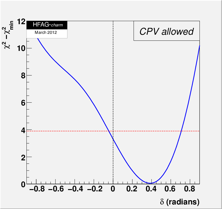


| Parameter | No | No direct | -allowed | -allowed 95% C.L. |
|---|---|---|---|---|
| Observable | ||
|---|---|---|
| 2.61 | 2.61 | |
| 0.00 | 2.61 | |
| Belle | 0.28 | 2.88 |
| Belle | 1.65 | 4.54 |
| Belle | 0.01 | 4.54 |
| Belle | 0.51 | 5.05 |
| BABAR | 2.97 | 8.02 |
| BABAR | 0.37 | 8.38 |
| 0.09 | 8.48 | |
| BABAR | 5.71 | 14.19 |
| BABAR | 2.22 | 16.40 |
| CLEOc | ||
| () | 7.28 | 23.68 |
| BABAR | 2.34 | 26.02 |
| BABAR | 1.30 | 27.31 |
| Belle | 4.12 | 31.44 |
| Belle | 1.35 | 32.79 |
| CDF | 0.39 | 33.17 |
| BABAR | 1.89 | 35.06 |
| Belle | 0.12 | 35.18 |
| CDF | 0.06 | 35.25 |
| LHCb | 0.37 | 35.62 |
8.1.4 Conclusions
From the fit results listed in Table 167 and shown in Figs. 65 and 66, we conclude the following:
- •
the experimental data consistently indicate that mesons undergo mixing. The no-mixing point is excluded at . The parameter differs from zero by , and differs from zero by . This mixing is presumably dominated by long-distance processes, which are difficult to calculate. Unless it turns out that [505], which is not indicated, it will probably be difficult to identify new physics from alone.
- •
Since is positive, the -even state is shorter-lived as in the - system. However, since also appears to be positive, the -even state is heavier, unlike in the - system.
- •
The LHCb and CDF experiments have obtained first evidence for direct in decays. Higher statistics measurements should be able to clarify this effect. There is no evidence for arising from - mixing () or from a phase difference between the mixing amplitude and a direct decay amplitude ().
8.2 Semileptonic decays
8.2.1 Introduction
Semileptonic decays of mesons involve the interaction of a leptonic current with a hadronic current. The latter is nonperturbative and cannot be calculated from first principles; thus it is usually parameterized in terms of form factors. The transition matrix element is written
| (187) |
where is the Fermi constant and is a CKM matrix element. The leptonic current is evaluated directly from the lepton spinors and has a simple structure; this allows one to extract information about the form factors (in ) from data on semileptonic decays [534]. Conversely, because there are no final-state interactions between the leptonic and hadronic systems, semileptonic decays for which the form factors can be calculated allow one to determine [2].
8.2.2 decays
When the final state hadron is a pseudoscalar, the hadronic current is given by
| (188) |
where and are the mass and four momentum of the parent meson, and are those of the daughter meson, and are form factors, and . Kinematics require that . The contraction results in terms proportional to [535], and thus for the last two terms in Eq. (188) are negligible. Considering that, only the form factor is relevant, the differential partial width is
| (189) |
where is the magnitude of the momentum of the final state hadron in the rest frame.
8.2.3 Form factor parameterizations
The form factor is traditionally parametrized with an explicit pole and a sum of effective poles:
| (190) |
where and are expansion parameters. The parameter is the mass of the lowest-lying resonance with the appropriate quantum numbers; this is expected to provide the largest contribution to the form factor for the transition. For example, for transitions the dominant resonance is expected to be , and thus .
Simple pole
Equation (190) can be simplified by neglecting the sum over effective poles, leaving only the explicit vector meson pole. This approximation is referred to as “nearest pole dominance” or “vector-meson dominance.” The resulting parameterization is
| (191) |
However, values of that give a good fit to the data do not agree with the expected vector meson masses [536]. To address this problem, the “modified pole” or Becirevic-Kaidalov (BK) parameterization [537] was introduced. is interpreted as the mass of an effective pole, higher than , thus it is expected that .
The parameterization takes the form
| (192) |
This parameterization has been used by several experiments to determine form factor parameters. Measured values of and are listed Tables 169 and 170 for and decays, respectively.
expansion
Several groups have advocated an alternative series expansion around some value to parameterize [538, 539, 540, 534]. This expansion is given in terms of a complex parameter , which is the analytic continuation of into the complex plane:
| (193) |
where and is the (arbitrary) value corresponding to . The physical region corresponds to .
The form factor is expressed as
| (194) |
where the factor accommodates sub-threshold resonances via
| (195) |
The “outer” function can be any analytic function, but a preferred choice (see, e.g. Refs. [538, 539, 541]) obtained from the Operator Product Expansion (OPE) is
| (196) | |||||
with . The OPE analysis provides a constraint upon the expansion coefficients, . These coefficients receive corrections, and thus the constraint is only approximate. However, the expansion is expected to converge rapidly since for () over the entire physical range, and Eq. (194) remains a useful parameterization.
8.2.4 Experimental techniques and results
Different techniques by several experiments have been used to measure D meson semileptonic decays with a pseudoscalar particle in the final state. The most recent results are provided by the Belle [542], BABAR [543] and CLEO-c [544],[545] collaborations. The BES III experiment has also reported preliminary results at the CHARM 2012 conference with 923 [546]. The Belle experiment fully reconstruct the D events from the continuum under the resonance, achieving a very good resolution () and low background level, but having a low efficiency. Using 282 , about 1300 and 115 signal semileptonic decays are isolated for each lepton flavour (e and ). The BABAR experiment uses a partial reconstruction technique where the semileptonic decays are tagged through the decay. The D direction and neutrino energy is obtained using information of the rest of the event. With 75 74000 signal events in the mode are obtained. The measurement of the Cabibbo suppressed mode has not been published yet. This technique provides larger statistics but higher background level and poorer resolution ( ranges from 66 to 219 ). In this case the measurement of the branching fraction is obtained by normalizing to the decay channel and can benefit from future improvements in the determination of this reference channel. The CLEO-c experiment uses two different methods to measure charm semileptonic decays. Tagged analyses [544] rely on the full reconstruction of events. One of the D mesons is reconstructed in a hadronic decay mode, the other in the semileptonic channel. The only missing particle is the neutrino so the resolution is very good and the background level very low. With the entire CLEO-c data sample, 818 , 14123 and 1374 signal events are reconstructed for the and channels, respectively, and 8467 and 838 for the and decays. Another technique without tagging the D meson in a hadronic mode (“untagged” in the following) has been also used by CLEO-c [545]. This method rests upon the association of the missing energy and momentum in an event with the neutrino four momentum, with the penalty of larger background as compared to the tagged method.
Previous measurements were also performed by CLEO III and FOCUS experiments. Events registered at the energy corresponding to an integrated luminosity of 7 were analyzed by CLEO III [547]. In the FOCUS fixed target photo-production experiment semileptonic events were obtained from the decay of a , and the kaon or pion was reconstructed in the muon channel.
Results of the hadronic form factor parameters by the different groups are given in Tables 169 and 170 for and .
| Expt. | Ref. | (GeV) | |
|---|---|---|---|
| CLEO III | [547] | ||
| FOCUS | [548] | ||
| Belle | [542] | ||
| BABAR | [543] | ||
| CLEO-c (tagged) | [544] | ||
| CLEO-c (untagged, ) | [545] | ||
| CLEO-c (untagged, ) | [545] | ||
| BESIII (prel) | [546] | ||
| Fermilab lattice/MILC/HPQCD | [549] | – |
| Expt. | Ref. | (GeV) | |
|---|---|---|---|
| CLEO III | [547] | ||
| FOCUS | [548] | – | |
| Belle | [542] | ||
| CLEO-c (tagged) | [544] | ||
| CLEO-c (untagged, ) | [545] | ||
| CLEO-c (untagged, ) | [545] | ||
| BESIII (prel) | [546] | ||
| Fermilab lattice/MILC/HPQCD | [549] | – |
The -expansion formalism has been used by BABAR [543] and CLEOc [544], [545]. BES III has also shown preliminary results[546] . Their fits used the first three terms of the expansion, and the results for the ratios and are listed in Tables 171 and 172. The CLEO III[547] and FOCUS[548] results listed are obtained by refitting their data using the full covariance matrix. The BABAR correlation coefficient listed is obtained by refitting their published branching fraction using their published covariance matrix.
These measurements correspond to using the standard outer function of Eq. (196) and . This choice of constrains to vary between
| Expt. | mode | Ref. | |||
| CLEO III | [547] | -0.99 | |||
| FOCUS | [548] | -0.97 | |||
| BABAR | [543] | -0.64 | |||
| CLEO-c (tagged) | [544] | -0.82 | |||
| CLEO-c (tagged) | [544] | -0.82 | |||
| CLEO-c (untagged) | [545] | -0.81 | |||
| CLEO-c (untagged) | [545] | -0.84 | |||
| BES III | [546] | ||||
| Combined | -0.82 |
| Expt. | mode | Ref. | |||
| CLEO-c (tagged) | [544] | 0 | -0.94 | ||
| CLEO-c (tagged) | [544] | 1 | -0.96 | ||
| CLEO-c (untagged) | [545] | -0.96 | |||
| CLEO-c (untagged) | [545] | -0.97 | |||
| BES III | [546] | 1 | |||
| Combined | -0.95 |
Tables 171 and 172 also list average values for and obtained from a 3D fit, taking the full correlations between , and into account, to CLEO III, FOCUS, BABAR, CLEO-c, and BES III data. Only the channels are entering in the fit. The fit is constrained by the branching fractions measured at Belle [542].
In the values quoted in Tables 169 and 171 the effect of radiative events has been taken into account slightly modifying the values from BABAR by correcting the numbers given in Tab. III of Ref. [543] by the shifts quoted in the last column of Tab. IV given in Ref. [543].
The of the combined fits are and for and , respectively. The correlation matrices are given in Tables 173 and 174.
| 1.000 | -0.446 | 0.672 | |
| -0.446 | 1.000 | -0.946 | |
| 0.672 | -0.946 | 1.000 |
| 1.000 | -0.088 | 0.433 | |
| -0.088 | 1.000 | -0.824 | |
| 0.433 | -0.824 | 1.000 |


| Experiment | Ref. | ||
|---|---|---|---|
| E691 (1989) | [552] | ||
| CLEO (1991) | [553] | ||
| CLEOII (1993) | [554] | ||
| CLEOII (1995) | [555] | ||
| E687 (1995) | [556] | ||
| E687 (1996) | [557] | ||
| BESII (2004) | [558] | ||
| CLEOIII (2005) | [547] | ||
| FOCUS (2005) | [548] | ||
| Belle (2006) | [542] | ||
| BABAR (2007) | [543] | ||
| CLEO-c (2008)(untagged) | [545] | ||
| CLEO-c (2009) (tagged) | [544] | ||
| BESIII (2012)(prel.) | [546] | ||
| Combined fit | |||
| HPQCD | [551][550] |
8.2.5 decays
When the final state hadron is a vector meson, the decay can proceed through both vector and axial vector currents, and four form factors are needed. The hadronic current is , where [535]
| (197) | |||||
| (198) | |||||
In this expression, is the daughter meson mass and
| (199) |
Kinematics require that . The differential partial width is
| (200) | |||||
where and are helicity amplitudes given by
| (201) | |||||
| (202) | |||||
is the three-momentum of the system, measured in the rest frame. The left-handed nature of the quark current manifests itself as . The differential decay rate for followed by the vector meson decaying into two pseudoscalars is
| (203) | |||||
where the angles , , and are defined in Fig. 68.

Ratios between the values of the hadronic form factors expressed at are usually introduced:
| (204) |
Table 176 lists measurements of and from several experiments. Most of measurements assume that the dependence of hadronic form factors is given by the simple pole anzats. The measurements are plotted in Fig. 69 which shows that they are all consistent.
| Experiment | Ref. | ||
|---|---|---|---|
| E691 | [559] | 2.0 0.6 0.3 | 0.0 0.5 0.2 |
| E653 | [560] | 2.00 0.33 0.16 | 0.82 0.22 0.11 |
| E687 | [561] | 1.74 0.27 0.28 | 0.78 0.18 0.11 |
| E791 (e) | [562] | 1.90 0.11 0.09 | 0.71 0.08 0.09 |
| E791 () | [563] | 1.840.110.09 | 0.750.080.09 |
| Beatrice | [564] | 1.45 0.23 0.07 | 1.00 0.15 0.03 |
| FOCUS | [565] | 1.5040.0570.039 | 0.8750.0490.064 |
| FOCUS | [566] | 1.7060.6770.342 | 0.9120.3700.104 |
| BABAR | [567] | ||
| BABAR | [568] | 1.6360.0670.038 | 0.7050.0560.029 |
| CLEO | [569] | 1.400.250.03 | 0.570.180.06 |

8.2.6 -wave component
In 2002 FOCUS reported [570] an asymmetry in the observed distribution. This is interpreted as evidence for an -wave component in the decay amplitude as follows. Since typically dominates over , the distribution given by Eq. (203) is, after integration over , roughly proportional to . Inclusion of a constant -wave amplitude of the form leads to an interference term proportional to ; this term causes an asymmetry in . When FOCUS fit their data including this -wave amplitude, they obtained GeV-1 and [565].
8.2.7 Model-independent form factor measurement
Subsequently the CLEO-c collaboration extracted the form factors , , and in a model-independent fashion directly as functions of [572] and also determined the -wave form factor via the interference term, despite the fact that the mass distribution appears dominated by the vector state. Their results are shown in Figs. 71 and 70. Plots in Fig. 71 clearly show that dominates over essentially the full range of , but especially at low . They also show that the transverse form factor (which can be related to is small (compared to Lattice Gauge Theory calculations) and suggest that the form factor ratio is large and negative.
The product is shown in Fig. 70 and clearly indicates the existence of , although it seems to fall faster with than . The other plots in that figure show that - and -wave versions of the -wave are not significant.


8.2.8 Detailed measurements of the decay channel
BABAR [567] has selected a large sample of signal events with a ratio from an analyzed integrated luminosity of . With four particles emitted in the final state, the differential decay rate depends on five variables. In addition to the four variables defined in previous sections there is , the mass squared of the system. Apart for this last variable, the reconstruction algorithm does not provide a high resolution on the other measured quantities and a multi-dimensional unfolding procedure is not used to correct for efficiency and resolution effects. Meanwhile these limitations still allow an essentially model independent measurement of the differential decay rate. This is because, apart for the and mass dependence of the form factors, angular distributions are fixed by kinematics. In addition, present accurate measurements of decays have shown that the dependence of the form factors can be well described by several models as long as the corresponding model parameter(s) are fitted on data. This is even more true in decays because the range is reduced. To analyze the decay channel it is assumed that all form factors have a variation given by the simple pole model and the effective pole mass value, , is fitted for the axial vector form factors. This value is compatible with expectations when comparing with the mass of charm mesons. Data are not sensitive to the effective mass of the vector form factor for which is used, nor to the effective pole mass of the scalar component for which is used. For the mass dependence of the form factors, a Breit-Wigner with a mass dependent width and a Blatt-Weisskopf damping factor is used. For the S-wave amplitude, considering what was measured in decays, a polynomial variation below the and a Breit-Wigner distribution, above are assumed. For the polynomial part, a linear term is sufficient to fit data.
It is verified that the variation of the S-wave phase is compatible with expectations from elastic scattering, according to the Watson theorem. At variance with elastic scattering, a negative relative sign between the S- and P-waves is measured; this is compatible with the previous theorem. In Fig. 72, the measured S-wave phase is compared with the phase of the elastic, , elastic phase for different values of the mass.

Contributions from other resonances decaying into are considered. A small signal from the is observed, compatible with expectations from decays and this component is included in the nominal fit. In total, 11 parameters are fitted in addition to the total number of signal events. They give a detailed description of the differential decay rate versus the 5 variables and corresponding matrices for statistical and systematic uncertainties are provided allowing to evaluate the compatibility of data with future theoretical expectations.
In Fig. 73 are compared measured values from CLEO-c of the products and with corresponding results from BABAR illustrating the difference in behaviour of the scalar component and the helicity zero P-wave form factor. For this comparison, plotted values from BABAR for the two distributions are equal to 1 at . The different behaviour of and can be explained by they different dependence in the variable.

Results of this analysis for the rates and few characteristics for S, P and D-waves are given in Table 177.
| Measurement | BABAR result |
|---|---|
| ( at 90 C.L.) | |
| ( at 90 C.L.) |
8.3 CP asymmetries
CP violation occurs if the decay rate for a particle differs from that of its CP-conjugate[574]. In general there are two classes of CP violation, termed indirect and direct[575]. Indirect CP violation refers to processes and arises in decays due to - mixing. It can occur as an asymmetry in the mixing itself, or it can result from interference between a decay amplitude arising via mixing and a non-mixed amplitude. Direct CP violation refers to processes and occurs in both charged and neutral decays. It results from interference between two different decay amplitudes (e.g., a penguin and tree amplitude) that have different weak (CKM) and strong phases5151 51 The weak phase difference will have opposite signs for and decays, while the strong phase difference will have the same sign. As a result, squaring the total amplitudes to obtain the decay rates gives interference terms having opposite sign, i.e., non-identical decay rates.. A difference in strong phases typically arises due to final-state interactions (FSI)[576]. A difference in weak phases arises from different CKM vertex couplings, as is often the case for spectator and penguin diagrams.
The CP asymmetry is defined as the difference between and partial widths divided by their sum:
| (205) |
However, to take into account differences in production rates between and (which would affect the number of respective decays observed), experiments usually normalize to a Cabibbo-favored mode. In this case there is the additional benefit that most corrections due to inefficiencies cancel out, reducing systematic uncertainties. An implicit assumption is that there is no measurable CP violation in the Cabibbo-favored normalizing mode. The CP asymmetry is calculated as
| (206) |
where (considering, for example, )
| (207) | |||||
| (208) |
In the case of and decays, measures direct CP violation; in the case of decays, measures direct and indirect CP violation combined. Values of for , and decays are listed in Tables 178, 179 and 180 respectively.
| Mode | Year | Collaboration | |
| 2008 | CLEOc [577] | ||
| 2010 | CLEOc [578] | ||
| 2010 | CLEOc [578] | ||
| 2010 | CLEOc [578] | ||
| 2010 | CLEOc [578] | ||
| 2011 | BABAR [579] | ||
| 2010 | Belle [580] | ||
| 2010 | CLEOc [578] | ||
| 2002 | FOCUS [581] | ||
| COMBOS average | |||
| 2010 | Belle [580] | ||
| 2010 | CLEOc [578] | ||
| 2002 | FOCUS [581] | ||
| COMBOS average | |||
| 1997 | E791 [582] | (stat.) | |
| 2010 | CLEOc [578] | ||
| 2007 | CLEO-c [583] | ||
| 2008 | CLEO-c [584] | ||
| 2005 | BABAR [585] | ||
| 2000 | FOCUS [586] | ||
| 1997 | E791 [582] | (stat.) | |
| 1994 | E687 [587] | (stat.) | |
| COMBOS average | |||
| 2007 | CLEOc [583] | ||
| 2007 | CLEOc [583] | ||
| 2005 | FOCUS [588] |
| Mode | Year | Collaboration | |
| 2012 | CDF [589] | ||
| 2008 | Belle [526] | ||
| 2008 | BABAR [525] | ||
| 2002 | CLEO [521] | ||
| 2000 | FOCUS [586] | ||
| 1998 | E791 [590] | ||
| COMBOS average | |||
| 2001 | CLEO [591] | (stat. and syst. combined) | |
| 2011 | Belle [592] | ||
| 2001 | CLEO [591] | (stat. and syst. combined) | |
| COMBOS average | |||
| 2011 | Belle [592] | ||
| 2011 | Belle [592] | ||
| 2001 | CLEO [591] | (stat. and syst. combined) | |
| 2012 | CDF [589] | ||
| 2008 | Belle [526] | ||
| 2008 | BABAR [525] | ||
| 2002 | CLEO [521] | ||
| 2000 | FOCUS [586] | ||
| 1998 | E791 [590] | ||
| 1995 | CLEO [593] | (stat.) | |
| 1994 | E687 [587] | (stat.) | |
| COMBOS average | |||
| 2008 | BABAR [594] | ||
| 2008 | Belle [595] | ||
| 2005 | CLEO [596] | ||
| COMBOS average | |||
| 2007 | CLEOc [583] | ||
| 2001 | CLEO [597] | (stat.) | |
| COMBOS average | |||
| 2005 | Belle [598] | (stat.) | |
| 2001 | CLEO [599] | (stat.) | |
| COMBOS average | |||
| 2004 | CLEO [600] | ||
| 2008 | BABAR [594] | ||
| 2005 | Belle [598] | (stat.) | |
| 2005 | FOCUS [588] |
| Mode | Year | Collaboration | |
| 2009 | CLEOc [601] | ||
| 2010 | CLEOc [578] | ||
| 2010 | CLEOc [578] | ||
| 2010 | Belle [580] | ||
| 2010 | CLEOc [578] | ||
| COMBOS average | |||
| 2010 | CLEOc [578] | ||
| 2010 | CLEOc [578] | ||
| 2010 | CLEOc [578] | ||
| 2010 | Belle [580] | ||
| 2010 | CLEOc [578] | ||
| COMBOS average | |||
| 2008 | CLEOc [602] | ||
| 2008 | CLEOc [602] | ||
| 2008 | CLEOc [602] | ||
| 2008 | CLEOc [602] | ||
| 2008 | CLEOc [602] |
8.4 -violating asymmetries
-violating asymmetries are measured using triple-product correlations and assuming the validity of the theorem. Triple-product correlations of the form , where , , and are spins or momenta, are odd under time reversal (T). For example, for decays, changes sign (i.e., is odd) under a T transformation. The corresponding quantity for is . Defining
| (209) |
for decay and
| (210) |
for decay, in the absence of strong phases either or indicates violation. In these expressions the ’s are partial widths. The asymmetry
| (211) |
tests for violation even with nonzero strong phases (see Refs. [603, 604, 605, 606, 607]). Values of for some , , and decay modes are listed in Table 181.
| Mode | Year | Collaboration | |
|---|---|---|---|
| 2010 | BABAR [608] | ||
| 2005 | FOCUS [588] | ||
| COMBOS average | |||
| 2010 | BABAR [609] | ||
| 2005 | FOCUS [588] | ||
| COMBOS average | |||
| 2010 | BABAR [609] | ||
| 2005 | FOCUS [588] | ||
| COMBOS average |
—————
8.5 World average for the decay constant
The Heavy Flavor Averaging Group has used measurements of the branching fractions [601, 610, 611] and [601, 612, 613, 610, 614, 611] from Belle, BABAR, and CLEO to calculate a world average (WA) value for the decay constant . We do not use older results from the ALEPH [615], BEATRICE [616], OPAL [617], and L3 [618] experiments as the errors are large and these measurements have some unknown systematic errors.
The value for is calculated using the formula
| (212) |
where or . For we use the WA values obtained below. The error on is calculated as follows: values for variables on the right-hand-side of Eq. (212) are sampled from Gaussian distributions having mean values equal to the central values and standard deviations equal to their respective errors. The resulting values of are plotted, and the r.m.s. of the distribution is taken as the errors on . The procedure is done separately for and ; the resulting two values for are averaged together using COMBOS [619], which accounts for correlations such as the values of , , and used5252 52 These values (taken from the PDG [21]) are ; GeV/; GeV/; and s. in Eq. (212). The result is plotted in Fig. 74. The WA value is
| (213) |
where the statistical and systematic errors are combined.

The WA value for is calculated from CLEOc [601], Belle [611], and BABAR [610] measurements of absolute branching fractions. These measurements are not normalized to decays as was done for earlier measurements, and thus they do not have uncertainties due to the non-resonant contribution. All input values and the result are plotted in Fig. 75. The WA value is .

The WA value for is also calculated from CLEOc, Belle, and BABAR measurements. CLEOc made separate measurements for [613], [601], and [612]; BABAR made separate measurements for [610] and [610, 614]; and Belle made separate measurements for , , and [611]. All input values and the result are plotted in Fig. 76. The WA value is .

8.6 Two-body hadronic decays and final state radiation
Branching fractions measurements for , and have reached sufficient precision to allow averages with relative uncertainties. At these precisions, Final State Radiation (FSR) must be treated correctly and consistently across the input measurements for the accuracy of the averages to match the precision. The sensitivity of measurements to FSR arises because of a tail in the distribution of radiated energy that extends to the kinematic limit. The tail beyond MeV causes typical selection variables like the hadronic invariant mass to shift outside the selection range dictated by experimental resolution (see Fig. 77). While the differential rate for the tail is small, the integrated rate amounts to several percent of the total rate because of the tail’s extent. The tail therefore translates directly into a several percent loss in experimental efficiency.
All measurements that include an FSR correction have a correction based on use of PHOTOS [620, 621, 622, 623] within the experiment’s Monte Carlo simulation. PHOTOS itself, however, has evolved, over the period spanning the set of measurements. In particular, incorporation of interference between radiation off of the two separate mesons has proceeded in stages: it was first available for particle–antiparticle pairs in version 2.00 (1993), and extended to any two body, all charged, final states in version 2.02 (1999). The effects of interference are clearly visible (Figure 77), and cause a roughly 30% increase in the integrated rate into the high energy photon tail. To evaluate the FSR correction incorporated into a given measurement, we must therefore note whether any correction was made, the version of PHOTOS used in correction, and whether the interference terms in PHOTOS were turned on.
8.6.1 Branching fraction corrections

Before averaging the measured branching fractions, the published results are updated, as necessary, to the FSR prediction of PHOTOS 2.15 with interference included. The correction will always shift a branching fraction to a higher value: with no FSR correction or with no interference term in the correction, the experimental efficiency determination will be biased high, and therefore the branching fraction will be biased low.
Most of the branching fraction analyses used the kinematic quantity sensitive to FSR in the candidate selection criteria. For the analyses at the , the variable was , the difference between the candidate energy and the beam energy (e.g., for ). In the remainder of the analyses, the relevant quantity was the reconstructed hadronic two-body mass . To correct we need only to evaluate the fraction of decays that FSR moves outside of the range accepted for the analysis.
The corrections were evaluated using an event generator (EvtGen [624]) that incorporates PHOTOS to simulate the portions of the decay process most relevant to the correction. We compared corrections determined both with and without smearing to account for experimental resolution. The differences were negligible, typically of order of a 1% of the correction itself. The immunity of the correction to resolution effects comes about because most of the long FSR-induced tail in, for example, the distribution resides well away from the selection boundaries. The smearing from resolution, on the other hand, mainly affects the distribution of events right at the boundary.
For measurements incorporating an FSR correction that did not include interference, we update by assessing the FSR-induced efficiency loss for both the PHOTOS version and configuration used in the analysis and our nominal version 2.15 with interference. For measurements that published their sensitivity to FSR, our generator-level predictions for the original efficiency loss agreed to within a few percent (of the correction). This agreement lends additional credence to the procedure.
Once the event loss from FSR in the most sensitive kinematic quantity is accounted for, the event loss from other quantities is very small. Analyses using tags, for example, showed little sensitivity to FSR in the reconstructed mass difference: for example, in . Because the effect of FSR tends to cancel in the difference of the reconstructed masses, this difference showed a much smaller sensitivity than the two body mass even before a two body mass requirement. In the analyses, the beam-constrained mass distributions () showed little further sensitivity.

The FOCUS [625] analysis of the branching ratios and obtained yields using fits to the two body mass distributions. FSR will both distort the low end of the signal mass peak, and will contribute a signal component to the low side tail used to estimate the background. The fitting procedure is not sensitive to signal events out in the FSR tail, which would be counted as part of the background.
A more complex toy Monte Carlo procedure was required to analyze the effect of FSR on the fitted yields, which were published with no FSR corrections applied. A detailed description of the procedure and results is available on the HFAG web page, and a brief summary is provided here. Determining the correction involved an iterative procedure in which samples of similar size to the FOCUS sample were generated and then fit using the FOCUS signal and background parameterizations. The MC parameterizations were tuned based on differences between the fits to the toy MC data and the FOCUS fits, and the procedure was repeated. These steps were iterated until the fit parameters matched the original FOCUS parameters.
| Experiment | result (rescaled) | correction [%] | PHOTOS |
|---|---|---|---|
| CLEO-c 07 (CC07) [583] | – | 2.15/Yes | |
| BABAR 07 (BB07) [626] | 0.69 | 2.02/No | |
| CLEO II 98 (CL98) [627] | 2.80 | none | |
| ALEPH 97 (AL97) [628] | 0.79 | 2.0/No | |
| ARGUS 94 (AR94) [629] | 2.33 | none | |
| CLEO II 93 (CL93) [630] | 0.38 | 2.0/No | |
| ALEPH 91 (AL91) [631] | 3.12 | none | |
| CLEO-c 10 (CC10) [578] | – | 2.15/Yes | |
| CDF 05 (CD05) [632] | – | 2.15/Yes | |
| FOCUS 02 (FO02) [625] | 3.10 | none | |
| CLEO-c 10 [578] | – | 2.15/Yes | |
| CDF 05 [632] | – | 2.15/Yes | |
| FOCUS 02 [625] | -1.12 | none | |
The toy MC samples for the first iteration were based on the generator-level distribution of , and , including the effects of FSR, smeared according to the original FOCUS resolution function, and on backgrounds thrown using the parameterization from the final FOCUS fits. For each iteration, 400 to 1600 individual data-sized samples were thrown and fit. The means of the parameters from these fits determined the corrections to the generator parameters for the following iteration. The ratio between the number of signal events generated and the final signal yield provides the required FSR correction in the final iteration. Only a few iterations were required in each mode. Figure 78 shows the FOCUS data, the published FOCUS fits, and the final toy MC parameterizations. The toy MC provides an excellent description of the data.
The corrections obtained to the individual FOCUS yields were for , for , and for . These corrections tend to cancel in the branching ratios, leading to corrections of 1.031 to , and 0.9888 for .
Table 182 summarizes the corrected branching fractions. The published FSR-related modeling uncertainties have been replaced by with a new, common, estimate based on the assumption that the dominant uncertainty in the FSR corrections come from the fact that the mesons are treated like structureless particles. No contributions from structure-dependent terms in the decay process (eg. radiation off individual quarks) are included in PHOTOS. Internal studies done by various experiments have indicated that in decay, the PHOTOS corrections agree with data at the 20-30% level. We therefore attribute a 25 uncertainty to the FSR prediction from potential structure-dependent contributions. For the other two modes, the only difference in structure is the final state valence quark content. While radiative corrections typically come in with a dependence, one would expect the additional contribution from the structure terms to come in on time scales shorter than the hadronization time scale. In this case, you might expect LambdaQCD to be the relevant scale, rather than the quark masses, and therefore that the amplitude is the same for the three modes. In treating the correlations among the measurements this is what we assume. We also assume that the PHOTOS amplitudes and any missing structure amplitudes are relatively real with constructive interference. The uncertainties largely cancel in the branching fraction ratios. For the final average branching fractions, the FSR uncertainty on dominates. Note that because of the relative sizes of FSR in the different modes, the branching ratio uncertainty from FSR is positively correlated with that for branching, while the branching ratio FSR uncertainty is negatively correlated.
The measurement of reference [633], the measurements of references [590] and [521] and the measurement of reference [521] are excluded from the branching fraction averages presented here. The measurements appear not to have incorporated any FSR corrections, and insufficient information is available to determine the 2-3% corrections that would be required.
| CC07 | BB07 | CL98 | AL97 | AR94 | CL93 | AL91 | FO02 | CD05 | CC10 | FO02 | CD05 | CC10 | ||||||||||||||
|---|---|---|---|---|---|---|---|---|---|---|---|---|---|---|---|---|---|---|---|---|---|---|---|---|---|---|
| CC07 | 1. | 000 | 0. | 106 | 0. | 044 | 0. | 064 | 0. | 023 | 0. | 025 | 0. | 018 | 0. | 053 | 0. | 078 | 0. | 052 | -0. | 015 | -0. | 025 | -0. | 065 |
| BB07 | 0. | 106 | 1. | 000 | 0. | 035 | 0. | 051 | 0. | 019 | 0. | 020 | 0. | 014 | 0. | 042 | 0. | 062 | 0. | 041 | -0. | 012 | -0. | 019 | -0. | 051 |
| CL98 | 0. | 044 | 0. | 035 | 1. | 000 | 0. | 021 | 0. | 008 | 0. | 298 | 0. | 006 | 0. | 017 | 0. | 026 | 0. | 017 | -0. | 005 | -0. | 008 | -0. | 021 |
| AL97 | 0. | 064 | 0. | 051 | 0. | 021 | 1. | 000 | 0. | 011 | 0. | 012 | 0. | 116 | 0. | 025 | 0. | 038 | 0. | 025 | -0. | 007 | -0. | 012 | -0. | 031 |
| AR94 | 0. | 023 | 0. | 019 | 0. | 008 | 0. | 011 | 1. | 000 | 0. | 004 | 0. | 003 | 0. | 009 | 0. | 014 | 0. | 009 | -0. | 003 | -0. | 004 | -0. | 011 |
| CL93 | 0. | 025 | 0. | 020 | 0. | 298 | 0. | 012 | 0. | 004 | 1. | 000 | 0. | 003 | 0. | 010 | 0. | 015 | 0. | 010 | -0. | 003 | -0. | 005 | -0. | 012 |
| AL91 | 0. | 018 | 0. | 014 | 0. | 006 | 0. | 116 | 0. | 003 | 0. | 003 | 1. | 000 | 0. | 007 | 0. | 010 | 0. | 007 | -0. | 002 | -0. | 003 | -0. | 009 |
| FO02 | 0. | 053 | 0. | 042 | 0. | 017 | 0. | 025 | 0. | 009 | 0. | 010 | 0. | 007 | 1. | 000 | 0. | 031 | 0. | 021 | -0. | 006 | -0. | 010 | -0. | 026 |
| CD05 | 0. | 078 | 0. | 062 | 0. | 026 | 0. | 038 | 0. | 014 | 0. | 015 | 0. | 010 | 0. | 031 | 1. | 000 | 0. | 031 | -0. | 009 | -0. | 014 | -0. | 038 |
| CC10 | 0. | 052 | 0. | 041 | 0. | 017 | 0. | 025 | 0. | 009 | 0. | 010 | 0. | 007 | 0. | 021 | 0. | 031 | 1. | 000 | -0. | 006 | -0. | 010 | -0. | 025 |
| FO02 | -0. | 015 | -0. | 012 | -0. | 005 | -0. | 007 | -0. | 003 | -0. | 003 | -0. | 002 | -0. | 006 | -0. | 009 | -0. | 006 | 1. | 000 | 0. | 003 | 0. | 007 |
| CD05 | -0. | 025 | -0. | 019 | -0. | 008 | -0. | 012 | -0. | 004 | -0. | 005 | -0. | 003 | -0. | 010 | -0. | 014 | -0. | 010 | 0. | 003 | 1. | 000 | 0. | 012 |
| CC10 | -0. | 065 | -0. | 051 | -0. | 021 | -0. | 031 | -0. | 011 | -0. | 012 | -0. | 009 | -0. | 026 | -0. | 038 | -0. | 025 | 0. | 007 | 0. | 012 | 1. | 000 |
8.6.2 Average branching fractions

The average branching fractions for , and are obtained from a single minimization procedure, in which the three branching fractions are floating parameters. The central values derive from a fit in which the covariance matrix is the sum of the covariance matrices for the statistical, systematic (excluding FSR) and FSR uncertainties. The statistical uncertainties are obtained from a fit using only the statistical covariance matrix. The systematic uncertainties are obtained from the quadrature uncertainties from a fit with statistical-only and statistical+systematic covariance matrices, and the FSR uncertainties on the averages from the quadrature differences in the uncertainties obtained from the nominal fit and a fit excluding the FSR uncertainties.
In forming the covariance matrix for the FSR uncertainties, the FSR uncertainties are treated as fully correlated (or anti-correlated) as described above. For the systematic covariance matrix, ALEPH’s systematic uncertainties in the parameter are treated as fully correlated between the ALEPH 97 and ALEPH 91 measurements. Similarly, the tracking efficiency uncertainties in the CLEO II 98 and the CLEO II 93 measurements are treated as fully correlated. Table 183 presents the correlation matrix for the nominal fit (stat.+syst.+FR).
The averaging procedure results in a final of 11.6 for 13-3 degrees of freedom. The branching fractions obtained are
The uncertainties, estimated as described above, are statistical, systematic (excluding FSR), and FSR modeling. The correlation coefficients from the fit using the total uncertainties are
| 1.00 | 0.72 | 0.78 | |
| 0.72 | 1.00 | 0.55 | |
| 0.78 | 0.55 | 1.00 |
| Modes | description | (%) | / (d.o.f.) |
|---|---|---|---|
| fit | |||
| PDG summer 2011 equivalent | 6.0 / (8-1) | ||
| drop Ref. [633] | 4.8 / (7-1) | ||
| add FSR corrections | 4.0 / (7-1) | ||
| add FSR correlations | 4.2 / (7-1) | ||
| all | – | 11.6 /(13-3) |
As the would suggest and Fig. 79 shows, the average value for and the input branching fractions agree very well. With the estimated uncertainty in the FSR modeling used here, the FSR uncertainty dominates the statistical uncertainty in the average, suggesting that experimental work in the near future should focus on verification of FSR with MeV. The and measurements inferred from the branching ration measurements also agree well (Fig. 80).
The average obtained here is approximately one statistical standard deviation higher than the 2011 PDG update average [6]. Table 184 shows the evolution from a fit similar to the PDG’s (no FSR corrections or correlations, reference [633] included) to the average presented here. There are two main contributions to the difference. The branching fraction in reference [633] is low, and its exclusion shifts the result upwards. The FSR corrections also shift the result upwards, as expected, and contribute the dominant shift of .


8.7 Direct violation
In decays of mesons, asymmetry measurements have contributions from both direct and indirect violation as discussed in Sec. 8.1. The contribution from indirect violation depends on the decay-time distribution of the data sample [532]. This section describes a combination of measurements that allows the extraction of the individual contributions of the two types of violation. At the same time, the level of agreement for a no--violation hypothesis is tested. The observables are:
| (214) |
where can be or , and
| (215) |
where are time-integrated asymmetries. The underlying theoretical parameters are:
| (216) |
where is the amplitude for [634]. We use the following relations between the observables and the underlying parameters [635]:
| (217) | |||||
| (218) |
The first relation constrains mostly indirect violation, and the direct violation contribution can differ for different final states. In the second relation, denotes the mean decay time in units of the lifetime; denotes the difference in quantity between and final states; and denotes the average for quantity . We neglect the last term in this relation as all three factors are or smaller, and thus this term is negligible with respect to the other two terms. Note that , and it is expected that because and are expected to have opposite signs.
A fit is performed in the plane vs. . For the BABAR result the difference of the quoted values for and is calculated, adding all uncertainties in quadrature. This may overestimate the systematic uncertainty for the difference as it neglects correlated errors; however, the result is conservative and the effect is small as all measurements are statistically limited. For all measurements, statistical and systematic uncertainties are added in quadrature when calculating the . We use the current world average value (see Sec. 8.1) and the measurements listed in Table 185.
| Year | Experiment | Results | Reference | ||
|---|---|---|---|---|---|
| 2007 | Belle | - | - | [502] | |
| 2008 | BABAR | - | - | [522] | |
| 2011 | LHCb | - | - | [524] | |
| 2008 | BABAR | ||||
| [525] | |||||
| 2008 | Belle | [526] | |||
| 2011 | LHCb | [527] | |||
| 2012 | CDF Prelim. | [529] |
The combination plot shows the measurements listed in Table 185 for and , where the bands represent intervals. The point of no violation (0,0) is shown as a filled circle, and two-dimensional CL, CL, and CL regions are plotted as ellipses. The best fit value is indicated by a cross showing the one-dimensional errors.

From the fit, the change in from the minimum value for the no- point (0,0) is , which corresponds to a CL of for two degrees of freedom. Thus the data are consistent with the no--violation hypothesis at only CL. The central values and errors for the individual parameters are
| (219) |
These results indicate that the origin of this violation lies in the difference between direct violation in the two final states, rather than in a common indirect violation.
8.8 Charm baryons
Here we summarizes present status of excited charm baryons, decaying strongly or electromagnetically: their masses (or mass difference between excited baryon and the corresponding ground state), natural widths, decay modes and presumably assigned quantum numbers. Table 186 summarizes the excited ’s. First two states, and are well established. Based on measured masses they are believed to be orbitally excited ’s with total momentum of light quarks L=1. Therefore, it’s quantum numbers are assigned to be and . Recently, their masses were precisely measured by CDF [636]: MeV/c2, MeV/c2. Next two states, and , were discovered by CLEO [637] in final state. They found that decays also through the mode. Later, BABAR [638] observed that this state has also decay mode. It is the first example where excited charm baryon decays into charm meson and light baryon. (Usually, excited charm baryons decay onto charm baryon and light mesons.) In that analysis BABAR observed for the first time else one state, , decaying into . By looking at final state, they found no signals which results in the conclusion that the and are really excited states, not . Belle reported the result of an angular analysis that favors the for the spin hypothesis. Moreover, the measured ratio of branching fractions combined with theoretical predictions based on HQS [430, 639] favoring even parity.
The open questions in the present excited family are the experimental determination of quantum numbers for almost all states and the nature of state: whether it is excited or .
| Charmed Baryon | Mode | Mass or , | Natural Width, | |
| Excited State | MeV/c2 | MeV/c2 | ||
| , | ||||
| , | ||||
| , | ?? | |||
| , , | ||||
| , | (experimental evidence) | |||
| , | ?? |
Table 187 summarizes the excited baryons. Triplet of baryons is well established. Recently CDF [636] precisely measured the masses and widths of the double charged and neutral members of this triplet to be MeV/c2, MeV/c2 and MeV/c2, MeV/c2, respectively. The short list of excited baryons completes the triplet of states observed by Belle [640]. Based on measured mass and theoretical predictions [641, 642] one can tentatively identify these states as members of the predicted triplet. From the study of resonant substructure in decays, BABAR found significant signal in with the mean value higher by about from obtained by Belle (see Table 187). The widths from measurements, Belle and BABAR, are consistent.
| Charmed Baryon | Mode | Mass or , | Natural Width, | |
| Excited State | MeV/c2 | MeV/c2 | ||
| @ 90 CL | ||||
| tentatively identified | ||||
| as members of the predicted | ||||
| isospin triplet | ||||
Table 188 summarizes the excited and baryons. Recently, the list of excited baryons have enriched by several states with masses above 2900 MeV/c2 and decaying into and . Some of these states are seen by both Belle [643] and BABAR [644] and are believed to be well-established, these are and . All others need to be confirmed or studied in more depth. These are seen in final state, found in final state, and claimed by BABAR [644] in final state.
The excited double charm baryon are seen by both BABAR [645] and Belle [646], the are in good agreement agreement in both experiments and consistent with most theoretical predictions [647, 648, 649, 650].
| Charmed Baryon | Mode | Mass or , | Natural Width, | |
| Excited State | MeV/c2 | MeV/c2 | ||
| , | ||||
| , | ||||
| ?? | ||||
| , , | ?? | |||
| ?? | ||||
| ?? | ||||
| , , | ?? | |||
| , , | ?? | |||
| ?? | ||||
Figure 82 shows the levels of excited charm baryons with the corresponding transitions between them or to the charm baryon ground states. Interesting feature recently discovered by BABAR and Belle is that now we know that transitions between families are possible (between and families of excited baryons). Also, highly excited baryons can decay into charm meson and proton.

8.9 Rare and forbidden decays
This section provides a summary of rare and forbidden charm decays in tabular form. The decay modes can be categorized as flavor-changing neutral currents, lepton-flavor-violating, lepton-number-violating, and both baryon- and lepton-number-violating decays. Figures 83-85 plot the upper limits for , , , and decays. Tables 189-192 give the corresponding numerical results. Some theoretical predictions are given in Refs. [651, 652, 653, 654, 655, 656].


| Decay | Limit | Experiment | Reference |
|---|---|---|---|
| 26.0 | CLEO II | [657] | |
| 2.2 | BABAR Preliminary | [658] | |
| 220.0 | CLEO | [659] | |
| 170.0 | Argus | [660] | |
| 130.0 | Mark3 | [661] | |
| 13.0 | CLEO II | [662] | |
| 8.19 | E789 | [663] | |
| 6.2 | E791 | [664] | |
| 1.2 | BABAR | [665] | |
| 0.079 | Belle | [666] | |
| 70.0 | Argus | [660] | |
| 44.0 | E653 | [667] | |
| 34.0 | CLEO II | [662] | |
| 15.6 | E789 | [663] | |
| 5.2 | E791 | [664] | |
| 2.0 | HERAb | [668] | |
| 1.3 | BABAR | [665] | |
| 0.21 | CDF | [669] | |
| 0.14 | Belle | [666] | |
| 0.011 | LHCb Preliminary | [670] | |
| 45.0 | CLEO II | [662] | |
| 540.0 | CLEO II | [662] | |
| 180.0 | E653 | [667] | |
| 110.0 | CLEO II | [662] | |
| 530.0 | CLEO II | [662] | |
| 370.0 | E791 | [671] | |
| 450.0 | CLEO | [659] | |
| 124.0 | E791 | [671] | |
| 100.0 | CLEO II | [662] | |
| 30.0 | E791 | [671] | |
| 810.0 | CLEO | [659] | |
| 490.0 | CLEO II | [662] | |
| 230.0 | E653 | [667] | |
| 22.0 | E791 | [671] | |
| 180.0 | CLEO II | [662] | |
| 830.0 | CLEO II | [662] | |
| 315.0 | E791 | [671] | |
| 59.0 | E791 | [671] | |
| 52.0 | CLEO II | [662] | |
| 33.0 | E791 | [671] | |
| 410.0 | CLEO II | [662] | |
| 31.0 | E791 | [671] | |
| 1700.0 | Mark3 | [672] | |
| 110.0 | CLEO II | [662] | |
| 670.0 | CLEO II | [662] | |
| 260.0 | E653 | [667] | |
| 385.0 | E791 | [671] | |
| 140.0 | CLEO II | [662] | |
| 47.0 | E791 | [671] | |
| 360.0 | E791 | [671] | |
| 1180.0 | CLEO II | [662] | |
| 24.0 | E791 | [671] | |
| 810.0 | E653 | [667] | |
| 270.0 | CLEO | [659] | |
| 120.0 | Mark3 | [673] | |
| 100.0 | Argus | [660] | |
| 19.0 | CLEO II | [662] | |
| 17.2 | E789 | [663] | |
| 8.1 | E791 | [664] | |
| 0.81 | BABAR | [665] | |
| 0.26 | Belle | [666] | |
| 86.0 | CLEO II | [662] | |
| 100.0 | CLEO II | [662] | |
| 15.0 | E791 | [671] | |
| 66.0 | E791 | [671] | |
| 49.0 | CLEO II | [662] | |
| 120.0 | CLEO II | [662] | |
| 180.0 | E791 | [671] | |
| 47.0 | E791 | [671] | |
| 34.0 | CLEO II | [662] | |
| 100.0 | CLEO II | [662] | |
| 550.0 | E791 | [671] | |
| 100.0 | CLEO II | [662] | |
| 83.0 | E791 | [671] | |
| 112.0 | E791 | [671] | |
| 29.0 | E791 | [671] | |
| 206.0 | E791 | [671] | |
| 390.0 | E791 | [671] | |
| 152.0 | E791 | [671] | |
| 94.0 | E791 | [671] | |
| 79.0 | E791 | [671] | |
| 218.0 | E791 | [671] | |
| 57.0 | E791 | [671] | |
| 10.0 | CLEO | [674] | |
| 11.0 | CLEO | [674] |
| Decay | Limit | Experiment | Reference |
|---|---|---|---|
| 110.0 | E687 | [675] | |
| 52.0 | E791 | [664] | |
| 5.9 | CLEO | [676] | |
| 1.1 | BABAR | [677] | |
| 220.0 | E653 | [667] | |
| 89.0 | E687 | [675] | |
| 15.0 | E791 | [664] | |
| 8.8 | FOCUS | [678] | |
| 6.5 | BABAR | [677] | |
| 3.9 | D0 | [679] | |
| 560.0 | E653 | [667] | |
| 200.0 | E687 | [675] | |
| 3.0 | CLEO | [676] | |
| 1.0 | BABAR | [677] | |
| 34.0 | E791 | [664] | |
| 110.0 | E687 | [675] | |
| 2.9 | BABAR | [677] | |
| 130.0 | E687 | [675] | |
| 3.6 | BABAR | [677] | |
| 68.0 | E791 | [664] | |
| 130.0 | E687 | [675] | |
| 1.2 | BABAR | [677] | |
| 120.0 | E687 | [675] | |
| 2.8 | BABAR | [677] | |
| 110.0 | E687 | [675] | |
| 96.0 | E791 | [664] | |
| 1.9 | BABAR | [677] | |
| 1.1 | CLEO | [676] | |
| 87.0 | E687 | [675] | |
| 17.0 | E791 | [664] | |
| 4.8 | FOCUS | [678] | |
| 2.0 | BABAR | [677] | |
| 110.0 | E687 | [675] | |
| 50.0 | E791 | [664] | |
| 560.0 | E653 | [667] | |
| 120.0 | E687 | [675] | |
| 3.5 | CLEO | [676] | |
| 0.9 | BABAR | [677] | |
| 320.0 | E653 | [667] | |
| 120.0 | E687 | [675] | |
| 13.0 | FOCUS | [678] | |
| 10.0 | BABAR | [677] | |
| 130.0 | E687 | [675] | |
| 850.0 | E653 | [667] |
| Decay | Limit | Experiment | Reference |
|---|---|---|---|
| 270.0 | E791 | [664] | |
| 22.0 | CLEO | [676] | |
| 13.0 | BABAR | [677] | |
| 430.0 | E653 | [667] | |
| 140.0 | E791 | [664] | |
| 43.0 | BABAR | [677] | |
| 26.0 | FOCUS | [678] | |
| 1600.0 | E791 | [664] | |
| 52.0 | CLEO | [676] | |
| 3.7 | BABAR | [677] | |
| 140.0 | E791 | [664] | |
| 36.0 | FOCUS | [678] | |
| 21.0 | BABAR | [677] | |
| 1400.0 | E653 | [667] | |
| 610.0 | E791 | [664] | |
| 12.0 | BABAR | [677] | |
| 20.0 | BABAR | [677] | |
| 630.0 | E791 | [664] | |
| 14.0 | BABAR | [677] | |
| 9.7 | BABAR | [677] | |
| 690.0 | E791 | [664] | |
| 18.0 | CLEO | [676] | |
| 4.1 | BABAR | [677] | |
| 430.0 | E653 | [667] | |
| 82.0 | E791 | [664] | |
| 29.0 | FOCUS | [678] | |
| 14.0 | BABAR | [677] | |
| 730.0 | E791 | [664] | |
| 630.0 | E791 | [664] | |
| 17.0 | CLEO | [676] | |
| 5.2 | BABAR | [677] | |
| 590.0 | E653 | [667] | |
| 180.0 | E791 | [664] | |
| 13.0 | FOCUS | [678] | |
| 680.0 | E791 | [664] | |
| 1400.0 | E653 | [667] |
9 Tau lepton properties
We present averages of a selection of physics quantities related to the tau lepton, where we follow the HFAG methodology [5] to improve the Review of Particle Physics (PDG) [6] results by:
- •
including a selection of reliable preliminary results, hence obtaining more up-to-date results;
- •
updating the experimental measurements value and systematic error when it depends on external parameters whose values and uncertainties are updated;
- •
taking into account the statistical correlation that is induced by the dependence from common systematic contributions.
All published statistical correlations are considered, and a selection of measurements, particularly the most precise and the most recent, were examined to obtain all the significant systematic dependencies. The HFAG techniques are most useful in the global fit of the tau branching fractions (Section 9.1). We use the branching fraction fit results to obtain updated lepton universality tests (Section 9.2) and updated determinations of with tau measurements (Section 9.4). Finally, we report in Section 9.5 the most up-to-date limits on the lepton-flavour-violating tau branching fractions.
9.1 Branching fractions fit
The measurements listed in Table 193 have been used in a minimum fit subject to the equality constraints that are listed either in the same table (where some fitted quantities and experimental measurements are expressed as ratios of fit quantities) or in Section 9.1.2. The fitted quantities and the measurements are labelled using the PDG [6] notation, where is an integer number, which matches the PDG notation for . We use to denote some additional branching fractions, as documented in the former HFAG report [5].
The fitted branching fractions consist on 40 “base nodes” and 45 derived branching fractions, described either as sum of base nodes (see Section 9.1.2) or as ratios of branching fractions (see Table 193). Furthermore, we define (see Section 9.1.2) as the sum of all the base modes, which correspond to all non-overlapping tau decay modes, and , which is the total branching fraction of the tau to modes with the strangeness quantum number equal to one.
The fitted HFAG-Tau averages are reported in Table 193. The fit has , corresponding to a confidence level . We use a total of 157 measurements and 47 constraint equations to fit 86 quantities. The fit is statistically consistent with the unitarity constraint, but the unitarity constraint is not applied.
In several cases, when it is statistically equivalent within the HFAG-Tau fitting procedure, for historical reasons the statistical and systematic errors are added in quadrature and are reported in the above table in the location of the statistical error, reporting zero as systematic error. A scale factor of 5.44 (as in the former report [5]) has been applied in the fit to the quoted errors of the two inconsistent measurements of by BABAR and Belle.
With respect to the end-of-2009 HFAG report [5], following comments by M. Davier [680], we have included 3 new modes:
along with the related measurements
the estimate
and the constraint
Furthermore, the following new measurements were added:
Finally, the constraint parameters (see Section 9.1.2) have been updated to the PDG 2011 results [6].
| Tau lepton branching fraction | Value | Exp. | Ref. |
|---|---|---|---|
| HFAG | Winter 2012 fit | ||
| ALEPH | [683] | ||
| DELPHI | [686] | ||
| L3 | [687] | ||
| OPAL | [688] | ||
| HFAG | Winter 2012 fit | ||
| ARGUS | [689] | ||
| BABAR | [690] | ||
| CLEO | [691] | ||
| HFAG | Winter 2012 fit | ||
| ALEPH | [683] | ||
| CLEO | [691] | ||
| DELPHI | [686] | ||
| L3 | [687] | ||
| OPAL | [692] | ||
| HFAG | Winter 2012 fit | ||
| DELPHI | [693] | ||
| L3 | [694] | ||
| OPAL | [695] | ||
| HFAG | Winter 2012 fit | ||
| ALEPH | [683] | ||
| CLEO | [691] | ||
| DELPHI | [696] | ||
| OPAL | [697] | ||
| HFAG | Winter 2012 fit | ||
| HFAG | Winter 2012 fit | ||
| BABAR | [690] | ||
| HFAG | Winter 2012 fit | ||
| ALEPH | [698] | ||
| CLEO | [699] | ||
| DELPHI | [700] | ||
| OPAL | [701] | ||
| HFAG | Winter 2012 fit | ||
| BABAR | [690] | ||
| HFAG | Winter 2012 fit | ||
| ALEPH | [683] | ||
| Belle | [702] | ||
| CLEO | [703] | ||
| DELPHI | [696] | ||
| L3 | [694] | ||
| OPAL | [697] | ||
| HFAG | Winter 2012 fit | ||
| HFAG | Winter 2012 fit | ||
| ALEPH | [698] | ||
| BABAR | [704] | ||
| CLEO | [699] | ||
| OPAL | [705] | ||
| HFAG | Winter 2012 fit | ||
| OPAL | [697] | ||
| HFAG | Winter 2012 fit | ||
| ALEPH | [683] | ||
| DELPHI | [696] | ||
| L3 | [694] | ||
| HFAG | Winter 2012 fit | ||
| CLEO | [706] | ||
| HFAG | Winter 2012 fit | ||
| HFAG | Winter 2012 fit | ||
| ALEPH | [698] | ||
| CLEO | [699] | ||
| HFAG | Winter 2012 fit | ||
| DELPHI | [696] | ||
| HFAG | Winter 2012 fit | ||
| ALEPH | [683] | ||
| L3 | [694] | ||
| HFAG | Winter 2012 fit | ||
| CLEO | [706] | ||
| HFAG | Winter 2012 fit | ||
| HFAG | Winter 2012 fit | ||
| ALEPH | [698] | ||
| HFAG | Winter 2012 fit | ||
| CLEO | [706] | ||
| HFAG | Winter 2012 fit | ||
| ALEPH | [683] | ||
| HFAG | Winter 2012 fit | ||
| CLEO | [699] | ||
| DELPHI | [700] | ||
| OPAL | [701] | ||
| HFAG | Winter 2012 fit | ||
| ALEPH | [681] | ||
| OPAL | [707] | ||
| HFAG | Winter 2012 fit | ||
| CLEO | [708] | ||
| HFAG | Winter 2012 fit | ||
| ALEPH | [698] | ||
| BABAR | [709] | ||
| Belle | [710] | ||
| L3 | [711] | ||
| OPAL | [712] | ||
| HFAG | Winter 2012 fit | ||
| ALEPH | [681] | ||
| ALEPH | [698] | ||
| CLEO | [708] | ||
| HFAG | Winter 2012 fit | ||
| OPAL | [712] | ||
| HFAG | Winter 2012 fit | ||
| CLEO | [708] | ||
| HFAG | Winter 2012 fit | ||
| ALEPH | [681] | ||
| ALEPH | [698] | ||
| BABAR | [713] | ||
| Belle | [685] | ||
| L3 | [711] | ||
| HFAG | Winter 2012 fit | ||
| ALEPH | [681] | ||
| ALEPH | [698] | ||
| Belle | [685] | ||
| CLEO | [708] | ||
| HFAG | Winter 2012 fit | ||
| OPAL | [712] | ||
| HFAG | Winter 2012 fit | ||
| ALEPH | [682] | ||
| HFAG | Winter 2012 fit | ||
| ALEPH | [681] | ||
| HFAG | Winter 2012 fit | ||
| ALEPH | [681] | ||
| CLEO | [708] | ||
| HFAG | Winter 2012 fit | ||
| ALEPH | [681] | ||
| HFAG | Winter 2012 fit | ||
| ALEPH | [682] | ||
| HFAG | Winter 2012 fit | ||
| ALEPH | [681] | ||
| HFAG | Winter 2012 fit | ||
| CELLO | [714] | ||
| L3 | [715] | ||
| TPC | [716] | ||
| HFAG | Winter 2012 fit | ||
| L3 | [717] | ||
| OPAL | [718] | ||
| HFAG | Winter 2012 fit | ||
| CLEO | [719] | ||
| DELPHI | [696] | ||
| HFAG | Winter 2012 fit | ||
| OPAL | [718] | ||
| HFAG | Winter 2012 fit | ||
| ALEPH | [683] | ||
| HFAG | Winter 2012 fit | ||
| BABAR | [720] | ||
| Belle | [721] | ||
| CLEO3 | [722] | ||
| HFAG | Winter 2012 fit | ||
| HFAG | Winter 2012 fit | ||
| ALEPH | [683] | ||
| CLEO | [719] | ||
| DELPHI | [696] | ||
| HFAG | Winter 2012 fit | ||
| CLEO | [723] | ||
| HFAG | Winter 2012 fit | ||
| HFAG | Winter 2012 fit | ||
| DELPHI | [696] | ||
| HFAG | Winter 2012 fit | ||
| ALEPH | [683] | ||
| HFAG | Winter 2012 fit | ||
| CLEO | [724] | ||
| HFAG | Winter 2012 fit | ||
| HFAG | Winter 2012 fit | ||
| CLEO | [725] | ||
| HFAG | Winter 2012 fit | ||
| CLEO | [726] | ||
| HFAG | Winter 2012 fit | ||
| CLEO | [726] | ||
| HFAG | Winter 2012 fit | ||
| TPC | [727] | ||
| HFAG | Winter 2012 fit | ||
| ALEPH | [728] | ||
| BABAR | [720] | ||
| Belle | [721] | ||
| CLEO3 | [722] | ||
| OPAL | [705] | ||
| HFAG | Winter 2012 fit | ||
| ALEPH | [728] | ||
| CLEO3 | [729] | ||
| HFAG | Winter 2012 fit | ||
| OPAL | [730] | ||
| TPC | [727] | ||
| HFAG | Winter 2012 fit | ||
| ALEPH | [728] | ||
| BABAR | [720] | ||
| Belle | [721] | ||
| CLEO3 | [722] | ||
| HFAG | Winter 2012 fit | ||
| CLEO | [726] | ||
| HFAG | Winter 2012 fit | ||
| ALEPH | [728] | ||
| CLEO3 | [729] | ||
| HFAG | Winter 2012 fit | ||
| CLEO | [726] | ||
| HFAG | Winter 2012 fit | ||
| BABAR | [720] | ||
| Belle | [721] | ||
| HFAG | Winter 2012 fit | ||
| CLEO | [731] | ||
| HRS | [732] | ||
| L3 | [717] | ||
| HFAG | Winter 2012 fit | ||
| ALEPH | [683] | ||
| ARGUS | [733] | ||
| BABAR | [734] | ||
| CLEO | [731] | ||
| DELPHI | [696] | ||
| HRS | [732] | ||
| OPAL | [735] | ||
| HFAG | Winter 2012 fit | ||
| ALEPH | [683] | ||
| CLEO | [725] | ||
| DELPHI | [696] | ||
| OPAL | [735] | ||
| HFAG | Winter 2012 fit | ||
| HFAG | Winter 2012 fit | ||
| ALEPH | [736] | ||
| Belle | [737] | ||
| CLEO | [738] | ||
| HFAG | Winter 2012 fit | ||
| BABAR | [684] | ||
| Belle | [737] | ||
| HFAG | Winter 2012 fit | ||
| Belle | [737] | ||
| CLEO | [739] | ||
| HFAG | Winter 2012 fit | ||
| Belle | [737] | ||
| CLEO | [739] | ||
| HFAG | Winter 2012 fit | ||
| BABAR | [740] | ||
| CLEO | [725] | ||
| HFAG | Winter 2012 fit | ||
| ALEPH | [736] | ||
| CLEO | [741] | ||
| HFAG | Winter 2012 fit | ||
| ALEPH | [742] | ||
| CLEO | [719] | ||
| HFAG | Winter 2012 fit | ||
| CLEO3 | [729] | ||
| HFAG | Winter 2012 fit | ||
| ALEPH | [736] | ||
| HFAG | Winter 2012 fit | ||
| CLEO | [724] | ||
| HFAG | Winter 2012 fit | ||
| HFAG | Winter 2012 fit | ||
| HFAG | Winter 2012 fit | ||
| HFAG | Winter 2012 fit | ||
| HFAG | Winter 2012 fit | ||
| HFAG | Winter 2012 fit | ||
| ALEPH | [683] | ||
| HFAG | Winter 2012 fit |
9.1.1 Correlation between base nodes uncertainties
The following tables report the correlation coefficients between base nodes, in percent.
| 23 | ||||||||||||||
| 7 | 5 | |||||||||||||
| 3 | 6 | 1 | ||||||||||||
| -13 | -14 | -12 | -3 | |||||||||||
| -0 | -1 | 2 | -1 | -16 | ||||||||||
| -5 | -5 | -7 | -1 | -40 | 2 | |||||||||
| 0 | 0 | -0 | -2 | 2 | -12 | -22 | ||||||||
| -4 | -3 | -8 | -1 | 0 | 3 | -36 | 6 | |||||||
| 0 | 0 | -0 | -1 | 2 | -12 | 4 | -19 | -29 | ||||||
| -5 | -4 | -11 | -2 | -9 | -0 | 6 | 0 | -42 | 0 | |||||
| -0 | -1 | 1 | 0 | -0 | 2 | -1 | 1 | -0 | 1 | -0 | ||||
| 0 | 0 | -1 | -1 | 1 | -8 | 3 | -12 | 4 | -12 | 0 | -6 | |||
| -0 | -1 | 1 | -0 | -0 | 0 | 1 | -2 | -2 | -2 | -0 | 0 | -3 | ||
| -0 | -0 | 0 | -0 | 0 | -3 | 1 | -5 | -1 | -5 | 0 | -0 | -7 | 30 | |
| 0 | 0 | -0 | 0 | -0 | 0 | -0 | 0 | 0 | 0 | 0 | -2 | -2 | -4 | |
| -0 | -0 | -0 | -0 | -0 | 0 | 0 | 0 | 0 | 0 | 0 | -0 | -0 | -0 | |
| 0 | 0 | 0 | 0 | 0 | 0 | -0 | 1 | -0 | 0 | -0 | -4 | -3 | -3 | |
| 0 | 0 | 0 | 0 | 0 | -0 | 0 | 0 | 0 | 0 | 0 | -0 | -0 | -0 | |
| -3 | -5 | 8 | 0 | -4 | 5 | -7 | -1 | -5 | -1 | -5 | 4 | -1 | 3 | |
| -6 | -6 | -7 | -1 | -9 | -1 | -1 | 0 | -1 | 0 | 3 | -1 | 0 | -1 | |
| -1 | -0 | -3 | -1 | -2 | -0 | -0 | 0 | 2 | 0 | 2 | -0 | 0 | -0 | |
| 1 | 1 | 2 | 0 | 1 | 1 | -0 | -0 | -0 | -0 | 0 | 1 | -0 | 1 | |
| -1 | -1 | 2 | 0 | -1 | 2 | -1 | -0 | -1 | -0 | -1 | 2 | -0 | 1 | |
| -0 | -0 | -0 | -0 | -0 | -0 | -0 | 0 | -0 | 0 | 0 | -0 | 0 | -0 | |
| 0 | 0 | 2 | 0 | 0 | 1 | -1 | -0 | -0 | -0 | -1 | 1 | -0 | 1 | |
| -1 | -1 | -1 | -0 | -1 | 0 | 0 | -0 | 0 | -0 | -1 | 0 | -0 | 0 | |
| 0 | 0 | 0 | 0 | 0 | 0 | -1 | -0 | 0 | -0 | -2 | 0 | -0 | 0 | |
| -0 | -0 | 1 | -0 | -0 | 1 | -0 | -1 | -0 | -1 | -0 | 1 | -0 | 1 | |
| 0 | 0 | 0 | 0 | 0 | 0 | -0 | -0 | 0 | -0 | -0 | 0 | -0 | 0 | |
| 0 | 0 | -0 | 0 | -0 | 0 | -0 | -0 | 0 | -0 | -0 | 0 | -0 | 0 | |
| -0 | -0 | -0 | -0 | -0 | 0 | -0 | -0 | -0 | -0 | 0 | -0 | -0 | -0 | |
| -1 | -0 | -3 | -1 | -2 | -0 | -1 | 0 | 2 | 0 | 2 | -0 | 0 | 0 | |
| -2 | -2 | -2 | -0 | -3 | -0 | -0 | 0 | -0 | 0 | 1 | -0 | 0 | -0 | |
| -0 | -0 | 0 | -0 | -0 | 0 | -0 | -0 | 0 | -0 | -0 | -0 | -0 | -0 | |
| -1 | -1 | 0 | 0 | -1 | -1 | -2 | 0 | -2 | 0 | -1 | -1 | -0 | -0 | |
| -0 | -0 | -0 | -0 | -0 | -0 | -0 | 0 | -0 | 0 | 0 | -0 | -0 | -0 | |
| 0 | 0 | 0 | 0 | 0 | 0 | 0 | 0 | 0 | 0 | 0 | 0 | 0 | 0 | |
| -2 | ||||||||||||||
| -0 | -0 | |||||||||||||
| -2 | -5 | -19 | ||||||||||||
| -0 | 0 | 0 | -0 | |||||||||||
| 1 | -0 | -0 | -0 | -0 | ||||||||||
| -0 | 0 | 0 | -0 | -0 | -19 | |||||||||
| 0 | -0 | -0 | 0 | 0 | -1 | -7 | ||||||||
| 0 | -0 | -0 | -0 | -0 | 2 | -2 | -1 | |||||||
| 0 | -0 | -0 | -0 | -0 | 14 | -4 | -0 | 1 | ||||||
| 0 | 0 | 0 | -0 | -0 | -0 | -2 | -0 | -0 | -0 | |||||
| 0 | -0 | -0 | -0 | -0 | 3 | -1 | -0 | 4 | 1 | -0 | ||||
| -0 | -0 | 0 | 0 | 0 | -0 | 0 | 1 | -36 | 0 | 0 | -11 | |||
| 0 | -0 | -0 | -0 | -0 | 1 | -0 | -5 | 0 | 0 | -0 | 0 | 0 | ||
| 0 | -0 | -0 | -0 | -0 | 2 | -0 | -0 | 0 | 1 | -0 | 1 | 0 | 4 | |
| 0 | -0 | -0 | -0 | -0 | 0 | -0 | -1 | 0 | 0 | -0 | 0 | 0 | 1 | |
| -0 | -0 | -0 | -0 | -0 | 0 | -0 | -0 | 0 | 0 | -0 | 0 | -0 | 2 | |
| 0 | 0 | 0 | -0 | -0 | 0 | 12 | 0 | 0 | 0 | -0 | 0 | 0 | 0 | |
| 0 | -0 | -0 | 0 | 0 | -1 | -11 | -64 | -1 | -0 | -0 | -0 | 1 | -0 | |
| -0 | 0 | 0 | -0 | -0 | -8 | -69 | -2 | -0 | -1 | 0 | -0 | 0 | -0 | |
| -0 | -0 | -0 | -0 | -0 | -1 | -0 | -0 | 0 | 1 | -0 | 0 | 0 | 0 | |
| -0 | 0 | 0 | -0 | -0 | 17 | -6 | -0 | -0 | -0 | -0 | -0 | -0 | -0 | |
| -0 | 0 | 0 | 0 | -0 | -1 | -19 | -0 | -0 | -0 | -2 | -0 | 0 | -0 | |
| 0 | 0 | 0 | 0 | 0 | 0 | 0 | 0 | 0 | 0 | 0 | 0 | 0 | 0 | |
| 1 | ||||||||||
| 1 | 0 | |||||||||
| 0 | 0 | -0 | ||||||||
| -0 | -0 | 0 | 0 | |||||||
| -0 | -0 | -0 | -14 | -3 | ||||||
| 0 | 0 | -0 | -0 | -0 | -0 | |||||
| -0 | -0 | -0 | -2 | -0 | -1 | 1 | ||||
| -1 | -0 | -0 | -58 | -0 | 9 | -0 | 1 | |||
| 0 | 0 | 0 | 0 | 0 | 0 | 0 | 0 | 0 | ||
9.1.2 Equality constraints
We use equality constraints that relate a branching fraction to a sum of branching fractions. As mentioned above, the tau branching fractions are denoted with labels. In the constraint relations we use the values of some non-tau branching fractions, denoted e.g. with the self-describing notation . We also use probabilities corresponding to modulus square amplitudes describing quantum mixtures of states such as , , , , denoted with e.g. . In the fit, all non-tau quantities are taken from the PDG 2011 [6] fits (when available) or averages, and are used without accounting for their uncertainties, which are however in general small with respect to the uncertainties on the tau branching fractions. The tau branching fractions are illustrated in Table 193. The equations in the following permit the computation of the values and uncertainties for branching fractions that are not listed in Table 193, once they are expressed as function of the quantities that are listed there. The following list does not include the (non-linear) constraints already introduced in Section 9.1, and illustrated in Table 193, where some measured branching fractions are expressed as ratios of “base” branching fractions.
9.1.3 Fit procedure
The fit procedure is functionally equivalent to the one employed in the former HFAG report [5] and consists in a minimum fit subject to linear and non-linear constraints. The fit code has been improved to automatize the treatment of non-linear constraints, which are iteratively Taylor-expanded to obtain numerically approximate linear constraints, which permit an analytical solution for the minimization when, as it happens in this case, the is a quadratic function of the fitted quantities.
9.2 Tests of lepton universality
In the Standard Model, the partial widths of a heavier lepton decaying to a lighter lepton are, neglecting neutrino masses and including radiative corrections [743],
where
Proper ratios of the above partial widths, corrected by the suitable above-illustrated factors to remove the dependencies from masses and radiative corrections, measure ratios of charged weak lepton coupling constants. Using the HFAG-Tau fit values where available and using PDG 2011 for the remaining quantities, we measure, accounting for the statistical correlations emerging from the HFAG-Tau fit:
Tau decays partial widths to hadrons compared to the same hadron decay to muons measure the tau-muon universality of charged weak couplings as follows:
where = or and the radiative corrections are and [744]. Using the HFAG-Tau data and PDG 2011 we measure:
Similar tests could be performed with decays to electrons, however they are less precise because the hadron two body decays to electrons are helicity-suppressed. Averaging the three ratios we obtain
accounting for statistical correlations.
9.3 Universality improved and
Following Ref. [745], we assume lepton universality to obtain a more precise experimental determination of using the tau branching fraction to muon and the tau lifetime, by averaging the direct measurement, the determination from assuming that hence (see also Section 9.2) , and from assuming that hence where . Accounting for statistical correlations, we obtain
We use to obtain the ratio
Here is obtained by summing all tau hadronic decay modes.
9.4 measurement
The CKM coefficient can be measured in several ways from the comparison of tau partial widths to strange and non-strange final states.
9.4.1 Inclusive tau partial width to strange
The tau hadronic partial width is the sum of the tau partial width to strange and to non-strange hadronic final states, . Dividing by the partial width to electron, , we obtain partial width ratios (which are equal to the respective branching fraction ratios) for which . In terms of such ratios, is measured as
| (220) |
where can be determined in the context of low energy QCD theory, partly relying on experimental low energy scattering data. We use [746], which induces a systematic error on that lies between two more recent estimates [747, 748].
In the following, we use the universality improved (see Section 9.3) to compute the ratios. The most direct experimental determination of and come from the tau inclusive branching fractions to hadronic and strange hadronic states, and . However often the total hadronic branching fraction has been replaced by the indirect but more precise expression (or similar expressions based on ), using unitarity, see for example the 2009 HFAG report [5]. We depart from this choice here, and we use the most direct determination of , for two reasons: first there is no significant statistical gain in the final errors, because of statistical correlations in the expression , and second the indirect determination of would absorb the effect of possible unobserved hadronic states entirely in , while they could also be strange final states.
With the above choices, using [749], using HFAG values of this report, including the above-mentioned , (see also Table 200), ) and the PDG 2011 averages, we obtain , which is lower than the unitarity CKM prediction , from . The uncertainty includes a systematic error contribution of 0.0010 from the theory uncertainty on ,
If we use the alternative above mentioned definitions of , the mismatch remains . Using a unitarity-constrained tau branching fraction fit, the mismatch remains . The discrepancy is close to the unconstrained fit result of the 2009 HFAG report, [5], and also to the from the HFAG-Tau 2011 intermediate document [750], based on a unitarity-constrained fit.
| Branching fraction | HFAG Winter 2012 fit |
|---|---|
9.4.2 from and from
We use the ratio of branching fractions to measure from the equation
In this ratio, the short-distance radiative corrections cancel. The term corresponds to the long-distance electroweak radiative correction factor for the process . Following Ref. [751], the ratio of radiative correction factors is estimated as , where the first ratio is [752] and the second ratio is [753], hence assuming independent errors . The ratio is estimated in lattice QCD to be [219]. We measure , below the CKM unitarity prediction.
We use the branching fraction to measure from the equation
where [219] is the kaon decay constant estimated with lattice QCD, and [754] accounts for the radiative corrections. We obtain , wich is below the CKM unitarity prediction. CODATA 2006 results [755] and PDG 2011 have been used for the physics constants.
9.4.3 from tau summary

We summarize the results reporting the values, the discrepancy with respect to the determination from CKM unitarity, and an illustration of the measurement method:
Thanks to the improved lattice QCD determination of [219], the uncertainty on has been significantly reduced with respect to the previous HFAG report. Averaging the three above determinations we obtain:
We could not find a published estimate of the correlation of the uncertainties on and , but even if we assume correlation, the uncertainty on does not change more than about . Figure 86 summarizes the results.
9.5 Upper limits on tau LFV branching fractions
We list in Table 201 the up-to-date upper limits on the tau LFV branching fractions.
| Decay mode | Category |
|
Exp. | Ref. | |||
|---|---|---|---|---|---|---|---|
| Belle | [757] | ||||||
| BABAR | [758] | ||||||
| Belle | [757] | ||||||
| BABAR | [758] | ||||||
| Belle | [759] | ||||||
| BABAR | [760] | ||||||
| Belle | [759] | ||||||
| BABAR | [760] | ||||||
| Belle | [759] | ||||||
| BABAR | [760] | ||||||
| Belle | [759] | ||||||
| BABAR | [760] | ||||||
| Belle | [759] | ||||||
| BABAR | [760] | ||||||
| Belle | [759] | ||||||
| BABAR | [760] | ||||||
| Belle | [761] | ||||||
| BABAR | [762] | ||||||
| Belle | [761] | ||||||
| BABAR | [762] | ||||||
| Belle | [763] | ||||||
| Belle | [763] | ||||||
| Belle | [764] | ||||||
| BABAR | [765] | ||||||
| Belle | [764] | ||||||
| BABAR | [765] | ||||||
| Belle | [764] | ||||||
| BABAR | [765] | ||||||
| Belle | [764] | ||||||
| BABAR | [765] | ||||||
| Belle | [764] | ||||||
| BABAR | [765] | ||||||
| Belle | [764] | ||||||
| BABAR | [765] | ||||||
| Belle | [764] | ||||||
| BABAR | [765] | ||||||
| Belle | [764] | ||||||
| BABAR | [765] | ||||||
| Belle | [764] | ||||||
| BABAR | [766] | ||||||
| Belle | [764] | ||||||
| BABAR | [766] | ||||||
| Belle | [767] | ||||||
| BABAR | [768] | ||||||
| Belle | [767] | ||||||
| BABAR | [768] | ||||||
| Belle | [767] | ||||||
| BABAR | [768] | ||||||
| Belle | [767] | ||||||
| BABAR | [768] | ||||||
| Belle | [767] | ||||||
| BABAR | [768] | ||||||
| Belle | [767] | ||||||
| BABAR | [768] | ||||||
| Belle | [769] | ||||||
| BABAR | [770] | ||||||
| Belle | [769] | ||||||
| BABAR | [770] | ||||||
| Belle | [769] | ||||||
| BABAR | [770] | ||||||
| Belle | [769] | ||||||
| BABAR | [770] | ||||||
| Belle | [769] | ||||||
| BABAR | [770] | ||||||
| Belle | [769] | ||||||
| BABAR | [770] | ||||||
| Belle | [769] | ||||||
| BABAR | [770] | ||||||
| Belle | [769] | ||||||
| BABAR | [770] | ||||||
| Belle | [761] | ||||||
| Belle | [761] | ||||||
| (L) | Belle | [769] | |||||
| (L) | BABAR | [770] | |||||
| (L) | Belle | [769] | |||||
| (L) | BABAR | [770] | |||||
| (L) | Belle | [769] | |||||
| (L) | BABAR | [770] | |||||
| (L) | Belle | [769] | |||||
| (L) | BABAR | [770] | |||||
| (L) | Belle | [769] | |||||
| (L) | BABAR | [770] | |||||
| (L) | Belle | [769] | |||||
| (L) | BABAR | [770] | |||||
| Belle | [771] | ||||||
| BABAR | [772] | ||||||
| Belle | [771] | ||||||
| BABAR | [772] | ||||||
| Belle | [771] | ||||||
| BABAR | [772] | ||||||
| Belle | [771] | ||||||
| BABAR | [772] | ||||||
Figure 87 summarizes the upper limits on the tau lepton-flavor-violating branching fractions.

10 Summary
This article provides updated world averages for -hadron properties using results available before the end of 2011. In some sections, results that appeared before the end of April 2012 are also included.
| -hadron lifetimes | |
|---|---|
| -hadron fractions | |
| in decays | |
| in decays | |
| , in decays | , |
| , at Tevatron | , |
| and mixing / parameters | |
| Measurements related to Unitarity Triangle angles | |
| Semileptonic decay parameters | |
|---|---|
| from | |
| from | |
| from | |
| from | |
| from | |
| Rare decays | |
| in bins of | see Table 142 |
| (90 % C.L.) | |
| mixing and parameters | |
|---|---|
| (no direct ) | |
| (no direct ) | |
| (no direct ) | |
| parameters, Lepton Universality, and | |
| from | |
| from | |
| from inclusive sum of strange branching fractions | |
| tau average |
Concerning -hadron lifetime and mixing averages, the most significant changes in the past two years are due to new results from the CDF, D0 and LHCb experiments, mainly in the sector. While the Tevatron experiments have updated some of their analyses with the full Run II data sample, LHCb has just entered the game and is taking the lead already with results based on the 2010–2011 data samples collected at the LHC. While the updated D0 like-sign dimuon asymmetry still deviates from the Standard Model prediction (with a significance increased to ), there is still no evidence of violation in either or mixing, with precisions on the semileptonic asymmetries reaching below the 1% level. However, the most impressive progress was achieved in the analysis of decays, where new or significantly improved results became recently available from CDF, D0 and LHCb. The non-zero decay width difference in the system is now firmly established, with a relative difference of . Its sign has also been determined by LHCb: the heavy state of the system lives longer than the light state, as expected in the Standard Model. In contrast, and despite the recent efforts from Belle, the relative decay width difference in the system, which has momentarily reached a slightly better absolute precision, is still consistent with zero. One the other hand, a quantum step has been achieved in the measurement of mixing-induced violation in decays proceeding through the transition: the corresponding weak phase has been pinned down to a precision below 0.1 radian and is so far compatible with the Standard Model expectation.
The measurement of from transitions such as has reached precision: . Measurements of the same parameter using different quark-level processes provide a consistency test of the Standard Model and allow insight into possible new physics. Recent improvements include the use of time-dependent Dalitz plot analyses of and to obtain violation parameters for , and . All results among hadronic penguin dominated decays are currently consistent with the Standard Model expectations. Among measurements related to the Unitarity Triangle angle , results from the system allow constraints at the level of . Knowledge of the third angle also continues to improve. Notwithstanding the well-known statistical issues in extracting the value of the angle itself, the world average values of the parameters in decays now show significant direct violation effects.
Regarding semileptonic meson decays, the factories Belle and BABAR continue to dominate the field and a number of results have appeared since the last update. Semileptonic decays remain a focus of interest for theorists: New lattice QCD and light-cone sum rule results help to understand exclusive transitions. Inclusive semileptonic decays are understood at full . Still, the experimental situation is not satisfactory: While inclusive and exclusive determinations of agree at the level of , inclusive and exclusive measurements of differ by three standard deviations. Clearly more effort on the experimental and theory side is required in the future.
The most important new measurements of rare decays are coming from the LHC. CMS and LHCb both have restrictive limits for the decays and . The sensitivity is approaching the SM expectations with no significant signals seen yet. LHCb has already produced many other results on a wide variety of decays as indicated in the tables in Sec. 7. Belle and BABAR continue to produce new results though their rates are dwindling. It will still be some years before we see new results from upgraded factories.
Many to charm results from LHCb are included in our report for the first time this year, combining with results from BABAR, Belle and CDF to yield a total of 632 measurements reported in 216 papers. The huge combined sample of hadrons allows measurements of decays to states with open or hidden charm content with unprecedented precision.
In the charm sector, - mixing is now well-established. Measurements of 38 separate observables from five experiments are input into a global fit for 10 underlying parameters, and the no-mixing hypothesis is excluded at a confidence level corresponding to . The mixing parameters and (see Table 204) differ from zero by and , respectively. The central values are consistent with mixing arising from long-distance processes, as predicted by theory; thus it will probably be difficult to identify new physics from mixing alone. The WA value for the observable is positive, which indicates that the -even state is shorter-lived as in the - system. However, also appears to be positive, which implies that the -even state is heavier, unlike in the - system. In the - system, there is no evidence for arising from mixing () or from a phase difference between the mixing amplitude and a direct decay amplitude (). However, both the LHCb and CDF experiments have obtained evidence for direct in and decays. These experiments measure nonzero values for the difference in direct between and modes, which requires that direct exists in at least one of them. Inputting these measurements into a global fit and also including measurements from Belle and BABAR gives with a significance greater than .
Concerning tau decays, in this report we include three new tau branching fraction measurements from the -factories, and we provide more information on the tau branching fraction fit. The calculation uses now a more complete set of tau branching fractions to strange final states, and thanks primarily to improvements in QCD lattice predictions, two tau determinations of have reduced errors. For the first time, we compute an average of all determinations with tau data.
11 Acknowledgments
We are grateful for the strong support of the Belle, BABAR, CLEO, CDF, D0 and LHCb collaborations, without whom this compilation of results and world averages would not have been possible. The success of these experiments in turn would not have been possible without the excellent operations of the KEKB, PEP-II, CESR, Tevatron and LHC accelerators, and fruitful collaborations between the accelerator groups and the experiments.
Our averages and this compilation have benefitted greatly from contributions to the Heavy Flavor Averaging Group from numerous individuals. We especially thank David Kirkby, Yoshihide Sakai, Simon Eidelman, Soeren Prell and Gianluca Cavoto for their past leadership of HFAG. We are grateful to Paolo Gambino for assistance with averages that appear in Chapter 5, to David Asner, David Cassel and Milind Purohit for significant contributions to Chapter 8, and to Michel Davier for providing valuable input to Chapter 9.
References
- [1] N. Cabibbo, Phys. Rev. Lett. 10, 531–533 (1963)
- [2] M. Kobayashi and T. Maskawa, Prog. Theor. Phys. 49, 652–657 (1973)
- [3] D. Abbaneo et al. (ALEPH, CDF, DELPHI, L3, OPAL, and SLD collaborations), arXiv:hep-ex/0009052 (2000), CERN-EP-2000-096
- [4] arXiv:hep-ex/0112028 (2001), CERN-EP-2001-050
- [5] D. Asner et al. (Heavy Flavor Averaging Group collaboration) (2010), arXiv:1010.1589 [hep-ex]
- [6] K. Nakamura et al. (Particle Data Group), J. Phys. G37, 075021 (2010), and 2011 partial update for the 2012 edition
- [7] B. Aubert et al. (BABAR collaboration), Phys. Rev. Lett. 94, 141801 (2005), arXiv:hep-ex/0412062
- [8] B. Aubert et al. (BABAR collaboration), Phys. Rev. D65, 032001 (2002), arXiv:hep-ex/0107025
- [9] B. Aubert et al. (BABAR collaboration), Phys. Rev. D69, 071101 (2004), arXiv:hep-ex/0401028
- [10] J. P. Alexander et al. (CLEO collaboration), Phys. Rev. Lett. 86, 2737–2741 (2001), arXiv:hep-ex/0006002
- [11] S. B. Athar et al. (CLEO collaboration), Phys. Rev. D66, 052003 (2002), arXiv:hep-ex/0202033
- [12] N. C. Hastings et al. (Belle collaboration), Phys. Rev. D67, 052004 (2003), arXiv:hep-ex/0212033
- [13] B. Aubert et al. (BABAR collaboration), Phys. Rev. Lett. 95, 042001 (2005), arXiv:hep-ex/0504001
- [14] B. Aubert et al. (BABAR collaboration), Phys. Rev. Lett. 96, 232001 (2006), arXiv:hep-ex/0604031
- [15] A. Sokolov et al. (Belle collaboration), Phys. Rev. D75, 071103 (2007), arXiv:hep-ex/0611026
- [16] B. Aubert et al. (BABAR collaboration), Phys. Rev. D78, 112002 (2008), arXiv:0807.2014 [hep-ex]
- [17] B. Barish et al. (CLEO collaboration), Phys. Rev. Lett. 76, 1570–1574 (1996)
- [18] A. Drutskoy et al. (Belle collaboration), Phys. Rev. D81, 112003 (2010), arXiv:1003.5885 [hep-ex]
- [19] G. S. Huang et al. (CLEO collaboration), Phys. Rev. D75, 012002 (2007), arXiv:hep-ex/0610035; this supersedes the results of Ref. [22]
- [20] A. Drutskoy et al. (Belle collaboration), Phys. Rev. Lett. 98, 052001 (2007), arXiv:hep-ex/0608015
- [21] J. Beringer et al. (Particle Data Group), Phys. Rev. D86, 010001 (2012)
- [22] M. Artuso et al. (CLEO collaboration), Phys. Rev. Lett. 95, 261801 (2005), arXiv:hep-ex/0508047
- [23] K. F. Chen et al. (Belle collaboration), Phys. Rev. Lett. 100, 112001 (2008), arXiv:0710.2577 [hep-ex]
- [24] I. Adachi et al. (Belle collaboration), Phys. Rev. Lett. 108, 032001 (2012), arXiv:1103.3419 [hep-ex]
- [25] R. Louvot, PhD thesis #5213, EPFL, Lausanne (2012), {http://dx.doi.org/10.5075/epfl-thesis-5213}
- [26] J. P. Lees et al. (BABAR collaboration), Phys. Rev. D85, 011101 (2012), arXiv:1110.5600 [hep-ex]
- [27] J. Li et al. (Belle collaboration), Phys. Rev. Lett. 106, 121802 (2011), arXiv:1102.2759 [hep-ex]
- [28] R. Louvot et al. (Belle collaboration), Phys. Rev. Lett. 102, 021801 (2009), arXiv:0809.2526 [hep-ex]
- [29] P. Abreu et al. (DELPHI collaboration), Phys. Lett. B289, 199–210 (1992)
- [30] P. D. Acton et al. (OPAL collaboration), Phys. Lett. B295, 357–370 (1992)
- [31] D. Buskulic et al. (ALEPH collaboration), Phys. Lett. B361, 221–233 (1995)
- [32] P. Abreu et al. (DELPHI collaboration), Z. Phys. C68, 375–390 (1995)
- [33] R. Barate et al. (ALEPH collaboration), Eur. Phys. J. C2, 197–211 (1998)
- [34] D. Buskulic et al. (ALEPH collaboration), Phys. Lett. B384, 449–460 (1996)
- [35] J. Abdallah et al. (DELPHI collaboration), Eur. Phys. J. C44, 299–309 (2005), arXiv:hep-ex/0510023
- [36] P. Abreu et al. (DELPHI collaboration), Z. Phys. C68, 541–554 (1995)
- [37] R. Barate et al. (ALEPH collaboration), Eur. Phys. J. C5, 205–227 (1998)
- [38] J. Abdallah et al. (DELPHI collaboration), Phys. Lett. B576, 29–42 (2003), arXiv:hep-ex/0311005
- [39] T. Affolder et al. (CDF collaboration), Phys. Rev. Lett. 84, 1663–1668 (2000), arXiv:hep-ex/9909011
- [40] T. Aaltonen et al. (CDF collaboration), Phys. Rev. D77, 072003 (2008), arXiv:0801.4375 [hep-ex]
- [41] T. Aaltonen et al. (CDF collaboration), Phys. Rev. D79, 032001 (2009), arXiv:0810.3213 [hep-ex]
- [42] F. Abe et al. (CDF collaboration), Phys. Rev. D60, 092005 (1999)
- [43] V. M. Abazov et al. (D0 collaboration), Phys. Rev. Lett. 99, 052001 (2007), arXiv:0706.1690 [hep-ex]
- [44] V. M. Abazov et al. (D0 collaboration), Phys. Rev. Lett. 101, 232002 (2008), arXiv:0808.4142 [hep-ex]
- [45] T. Aaltonen et al. (CDF collaboration), Phys. Rev. D80, 072003 (2009), arXiv:0905.3123 [hep-ex]
- [46] R. Aaij et al. (LHCb collaboration), Phys. Rev. D85, 032008 (2012), arXiv:1111.2357 [hep-ex]; the full covariance matrix of the measurements is available at {https://cdsweb.cern.ch/record/1390838}
- [47] R. Aaij et al. (LHCb collaboration), Phys. Rev. Lett. 107, 211801 (2011), arXiv:1106.4435 [hep-ex]
- [48] S. Schael et al. (ALEPH, CDF, DELPHI, L3, OPAL, and SLD collaborations, LEP electroweak working group, SLD electroweak and heavy flavour working groups), Phys. Rept. 427, 257 (2006), arXiv:hep-ex/0509008; we use the average given in Eq. 5.39 of this paper, obtained from a 10-parameter global fit of all electroweak data where the asymmetry measurements have been excluded
- [49] V. M. Abazov et al. (D0 collaboration), Phys. Rev. D74, 092001 (2006), arXiv:hep-ex/0609014
- [50] CDF collaboration, CDF note 10335, 27 January 2011, {http://www-cdf.fnal.gov/physics/new/bottom/110127.blessed-chibar/}
- [51] D. Acosta et al. (CDF collaboration), Phys. Rev. D69, 012002 (2004), arXiv:hep-ex/0309030; this supersedes the value of Ref. [224]
- [52] M. A. Shifman and M. B. Voloshin, Sov. Phys. JETP 64, 698 (1986)
- [53] J. Chay, H. Georgi, and B. Grinstein, Phys. Lett. B247, 399–405 (1990)
- [54] I. I. Bigi, N. G. Uraltsev, and A. I. Vainshtein, Phys. Lett. B293, 430–436 (1992), arXiv:hep-ph/9207214
- [55] erratum Phys. Lett. B297, 477 (1992)
- [56] I. I. Bigi, arXiv:hep-ph/9508408 (1995)
- [57] G. Bellini, I. I. Bigi, and P. J. Dornan, Phys. Rept. 289, 1–155 (1997)
- [58] M. Ciuchini, E. Franco, V. Lubicz, and F. Mescia, Nucl. Phys. B625, 211–238 (2002), arXiv:hep-ph/0110375
- [59] M. Beneke, G. Buchalla, C. Greub, A. Lenz, and U. Nierste, Nucl. Phys. B639, 389–407 (2002), arXiv:hep-ph/0202106
- [60] E. Franco, V. Lubicz, F. Mescia, and C. Tarantino, Nucl. Phys. B633, 212–236 (2002), arXiv:hep-ph/0203089
- [61] C. Tarantino, Eur. Phys. J. C33, s895–s899 (2004), arXiv:hep-ph/0310241
- [62] F. Gabbiani, A. I. Onishchenko, and A. A. Petrov, Phys. Rev. D68, 114006 (2003), arXiv:hep-ph/0303235
- [63] F. Gabbiani, A. I. Onishchenko, and A. A. Petrov, Phys. Rev. D70, 094031 (2004), arXiv:hep-ph/0407004
- [64] L. Di Ciaccio et al. (1996), internal note by former lifetime working group, {http://lepbosc.web.cern.ch/LEPBOSC/lifetimes/ps/final_blife.ps}
- [65] D. Buskulic et al. (ALEPH collaboration), Phys. Lett. B314, 459–470 (1993)
- [66] P. Abreu et al. (DELPHI collaboration), Z. Phys. C63, 3–16 (1994)
- [67] P. Abreu et al. (DELPHI collaboration), Phys. Lett. B377, 195–204 (1996)
- [68] J. Abdallah et al. (DELPHI collaboration), Eur. Phys. J. C33, 307–324 (2004), arXiv:hep-ex/0401025
- [69] M. Acciarri et al. (L3 collaboration), Phys. Lett. B416, 220–232 (1998)
- [70] K. Ackerstaff et al. (OPAL collaboration), Z. Phys. C73, 397–408 (1997)
- [71] K. Abe et al. (SLD collaboration), Phys. Rev. Lett. 75, 3624–3628 (1995), arXiv:hep-ex/9511005
- [72] D. Buskulic et al. (ALEPH collaboration), Phys. Lett. B369, 151–162 (1996)
- [73] P. D. Acton et al. (OPAL collaboration), Z. Phys. C60, 217–228 (1993)
- [74] F. Abe et al. (CDF collaboration), Phys. Rev. D57, 5382–5401 (1998)
- [75] ATLAS collaboration, ATLAS note ATLAS-CONF-2011-145, 11 October 2011, {https://cdsweb.cern.ch/record/1389455}
- [76] R. Barate et al. (ALEPH collaboration), Phys. Lett. B492, 275–287 (2000), arXiv:hep-ex/0008016
- [77] D. Buskulic et al. (ALEPH collaboration), Z. Phys. C71, 31–44 (1996)
- [78] P. Abreu et al. (DELPHI collaboration), Z. Phys. C68, 13–24 (1995)
- [79] W. Adam et al. (DELPHI collaboration), Z. Phys. C68, 363–374 (1995)
- [80] P. Abreu et al. (DELPHI collaboration), Z. Phys. C74, 19–32 (1997)
- [81] M. Acciarri et al. (L3 collaboration), Phys. Lett. B438, 417–429 (1998)
- [82] R. Akers et al. (OPAL collaboration), Z. Phys. C67, 379–388 (1995)
- [83] G. Abbiendi et al. (OPAL collaboration), Eur. Phys. J. C12, 609–626 (2000), arXiv:hep-ex/9901017
- [84] G. Abbiendi et al. (OPAL collaboration), Phys. Lett. B493, 266–280 (2000), arXiv:hep-ex/0010013
- [85] K. Abe et al. (SLD collaboration), Phys. Rev. Lett. 79, 590–596 (1997)
- [86] F. Abe et al. (CDF collaboration), Phys. Rev. D58, 092002 (1998), arXiv:hep-ex/9806018
- [87] D. E. Acosta et al. (CDF collaboration), Phys. Rev. D65, 092009 (2002)
- [88] T. Aaltonen et al. (CDF collaboration), Phys. Rev. Lett. 106, 121804 (2011), arXiv:1012.3138 [hep-ex]
- [89] these results replace the and lifetime measurements of A. Abulencia et al. (CDF collaboration), Phys. Rev. Lett. 98, 122001 (2007), arXiv:hep-ex/0609021, as well as the lifetime measurement of Ref. [312]
- [90] V. M. Abazov et al. (D0 collaboration), Phys. Rev. Lett. 102, 032001 (2009), arXiv:0810.0037 [hep-ex]
- [91] this replaces V. M. Abazov et al. (D0 collaboration), Phys. Rev. Lett. 95, 171801 (2005), arXiv:hep-ex/0507084
- [92] V. M. Abazov et al. (D0 collaboration), Phys. Rev. D85, 112003 (2012), arXiv:1204.2340 [hep-ex]
- [93] this replaces V. M. Abazov et al. (D0 collaboration), Phys. Rev. Lett. 99, 142001 (2007), arXiv:0704.3909 [hep-ex]
- [94] and V. M. Abazov et al. (D0 collaboration), Phys. Rev. Lett. 94, 102001 (2005), arXiv:hep-ex/0410054
- [95] B. Aubert et al. (BABAR collaboration), Phys. Rev. Lett. 87, 201803 (2001), arXiv:hep-ex/0107019
- [96] B. Aubert et al. (BABAR collaboration), Phys. Rev. Lett. 89, 011802 (2002), arXiv:hep-ex/0202005
- [97] erratum Phys. Rev. Lett. 89, 169903 (2002)
- [98] B. Aubert et al. (BABAR collaboration), Phys. Rev. D67, 072002 (2003), arXiv:hep-ex/0212017
- [99] B. Aubert et al. (BABAR collaboration), Phys. Rev. D67, 091101 (2003), arXiv:hep-ex/0212012
- [100] B. Aubert et al. (BABAR collaboration), Phys. Rev. D73, 012004 (2006), arXiv:hep-ex/0507054
- [101] K. Abe et al. (Belle collaboration), Phys. Rev. D71, 072003 (2005), arXiv:hep-ex/0408111
- [102] ATLAS collaboration, ATLAS note ATLAS-CONF-2011-092, 5 July 2011, {https://cdsweb.cern.ch/record/1363779}
- [103] LHCb collaboration, LHCb note LHCb-CONF-2011-001, 25 March 2011, {https://cdsweb.cern.ch/record/1328683}
- [104] T. Aaltonen et al. (CDF collaboration), Phys. Rev. D83, 032008 (2011), arXiv:1004.4855 [hep-ex]
- [105] V. M. Abazov et al. (D0 collaboration), Phys. Rev. Lett. 94, 182001 (2005), arXiv:hep-ex/0410052
- [106] CDF collaboration, CDF note 7514, 1 March 2005, {http://www-cdf.fnal.gov/physics/new/bottom/050224.blessed-bsemi-life/}
- [107] CDF collaboration, CDF note 7386, 23 March 2005, {http://www-cdf.fnal.gov/physics/new/bottom/050303.blessed-bhadlife/}
- [108] A. Lenz and U. Nierste (2011), arXiv:1102.4274 [hep-ph]
- [109] this updates the results of A. Lenz and U. Nierste, JHEP 06, 072 (2007), arXiv:hep-ph/0612167
- [110] M. Beneke, G. Buchalla, C. Greub, A. Lenz, and U. Nierste, Phys. Lett. B459, 631–640 (1999), arXiv:hep-ph/9808385
- [111] R. Aaij et al. (LHCb collaboration) (2012), arXiv:1202.4717 [hep-ex], to appear in Phys. Rev. Lett.
- [112] D. Buskulic et al. (ALEPH collaboration), Phys. Lett. B377, 205–221 (1996)
- [113] F. Abe et al. (CDF collaboration), Phys. Rev. D59, 032004 (1999), arXiv:hep-ex/9808003
- [114] P. Abreu et al. (DELPHI collaboration), Eur. Phys. J. C16, 555 (2000), arXiv:hep-ex/0107077
- [115] K. Ackerstaff et al. (OPAL collaboration), Phys. Lett. B426, 161–179 (1998), arXiv:hep-ex/9802002
- [116] V. M. Abazov et al. (D0 collaboration), Phys. Rev. Lett. 97, 241801 (2006), arXiv:hep-ex/0604046
- [117] T. Aaltonen et al. (CDF collaboration), Phys. Rev. Lett. 107, 272001 (2011), arXiv:1103.1864 [hep-ex]
- [118] we consider that these results supersede those from the old CDF note 7386 [107], although the lifetime analysis of one of the modes () has not been updated
- [119] R. Barate et al. (ALEPH collaboration), Eur. Phys. J. C4, 367–385 (1998)
- [120] P. Abreu et al. (DELPHI collaboration), Eur. Phys. J. C18, 229–252 (2000), arXiv:hep-ex/0105077
- [121] K. Ackerstaff et al. (OPAL collaboration), Eur. Phys. J. C2, 407–416 (1998), arXiv:hep-ex/9708023
- [122] V. M. Abazov et al. (D0 collaboration), Phys. Rev. Lett. 94, 042001 (2005), arXiv:hep-ex/0409043
- [123] R. Barate et al. (ALEPH collaboration), Phys. Lett. B486, 286–299 (2000)
- [124] R. Aaij et al. (LHCb collaboration), Phys. Lett. B707, 349–356 (2012), arXiv:1111.0521 [hep-ex]
- [125] LHCb collaboration, LHCb note LHCb-CONF-2012-001, 7 March 2012, {http://cdsweb.cern.ch/record/1422996}
- [126] T. Aaltonen et al. (CDF collaboration), Phys. Rev. D84, 052012 (2011), arXiv:1106.3682 [hep-ex]
- [127] K. Hartkorn and H. G. Moser, Eur. Phys. J. C8, 381–383 (1999)
- [128] CDF collaboration, CDF note 7757, 13 August 2005, {http://www-cdf.fnal.gov/physics/new/bottom/050707.blessed-bs-semi_life/}
- [129] CDF collaboration, CDF note 8524, 7 March 2007, {http://www-cdf.fnal.gov/physics/new/bottom/061130.blessed-bh-lifetime_v2/}
- [130] all these preliminary results are superseded by Ref. [88, *Abulencia:2006dr_mod_cont, 312] except those on
- [131] D. Tonelli (for the CDF collaboration), arXiv:hep-ex/0605038 (2006)
- [132] F. Abe et al. (CDF collaboration), Phys. Rev. Lett. 81, 2432–2437 (1998), arXiv:hep-ex/9805034
- [133] CDF collaboration, CDF note 9294, 28 April 2008, {http://www-cdf.fnal.gov/physics/new/bottom/080327.blessed-BC_LT_SemiLeptonic/}
- [134] this replaces A. Abulencia et al. (CDF collaboration), Phys. Rev. Lett. 97, 012002 (2006), arXiv:hep-ex/0603027
- [135] V. M. Abazov et al. (D0 collaboration), Phys. Rev. Lett. 102, 092001 (2009), arXiv:0805.2614 [hep-ex]
- [136] A. Abulencia et al. (CDF collaboration), Phys. Rev. Lett. 96, 082002 (2006), arXiv:hep-ex/0505076
- [137] T. Aaltonen et al. (CDF collaboration), Phys. Rev. Lett. 100, 182002 (2008), arXiv:0712.1506 [hep-ex]
- [138] CDF collaboration, CDF note 10533, 21 August 2011, {http://www-cdf.fnal.gov/physics/new/bottom/110804.blessed-bc-lifetime/}
- [139] D. E. Acosta et al. (CDF collaboration), Phys. Rev. Lett. 96, 202001 (2006), arXiv:hep-ex/0508022
- [140] D. Buskulic et al. (ALEPH collaboration), Phys. Lett. B365, 437–447 (1996)
- [141] P. Abreu et al. (DELPHI collaboration), Eur. Phys. J. C10, 185–199 (1999)
- [142] F. Abe et al. (CDF collaboration), Phys. Rev. Lett. 77, 1439–1443 (1996)
- [143] T. Aaltonen et al. (CDF collaboration), Phys. Rev. Lett. 104, 102002 (2010), arXiv:0912.3566 [hep-ex]
- [144] V. M. Abazov et al. (D0 collaboration), Phys. Rev. Lett. 99, 182001 (2007), arXiv:0706.2358 [hep-ex]
- [145] P. Abreu et al. (DELPHI collaboration), Z. Phys. C71, 199–210 (1996)
- [146] R. Akers et al. (OPAL collaboration), Z. Phys. C69, 195–214 (1996)
- [147] M. Beneke, G. Buchalla, and I. Dunietz, Phys. Rev. D54, 4419–4431 (1996), arXiv:hep-ph/9605259
- [148] Y.-Y. Keum and U. Nierste, Phys. Rev. D57, 4282–4289 (1998), arXiv:hep-ph/9710512
- [149] M. B. Voloshin, Phys. Rept. 320, 275–285 (1999), arXiv:hep-ph/9901445
- [150] B. Guberina, B. Melic, and H. Stefancic, Phys. Lett. B469, 253–258 (1999), arXiv:hep-ph/9907468
- [151] M. Neubert and C. T. Sachrajda, Nucl. Phys. B483, 339–370 (1997), arXiv:hep-ph/9603202
- [152] I. I. Bigi, M. A. Shifman, and N. Uraltsev, Ann. Rev. Nucl. Part. Sci. 47, 591–661 (1997), arXiv:hep-ph/9703290 [hep-ph]
- [153] N. G. Uraltsev, Phys. Lett. B376, 303–308 (1996), arXiv:hep-ph/9602324
- [154] D. Pirjol and N. Uraltsev, Phys. Rev. D59, 034012 (1999), arXiv:hep-ph/9805488
- [155] P. Colangelo and F. De Fazio, Phys. Lett. B387, 371–378 (1996), arXiv:hep-ph/9604425
- [156] M. Di Pierro, C. T. Sachrajda, and C. Michael (UKQCD collaboration), Phys. Lett. B468, 143 (1999), arXiv:hep-lat/9906031
- [157] D. Buskulic et al. (ALEPH collaboration), Z. Phys. C75, 397–407 (1997)
- [158] P. Abreu et al. (DELPHI collaboration), Z. Phys. C76, 579–598 (1997)
- [159] J. Abdallah et al. (DELPHI collaboration), Eur. Phys. J. C28, 155–173 (2003), arXiv:hep-ex/0303032
- [160] M. Acciarri et al. (L3 collaboration), Eur. Phys. J. C5, 195–203 (1998)
- [161] K. Ackerstaff et al. (OPAL collaboration), Z. Phys. C76, 417–423 (1997), arXiv:hep-ex/9707010
- [162] K. Ackerstaff et al. (OPAL collaboration), Z. Phys. C76, 401–415 (1997), arXiv:hep-ex/9707009
- [163] G. Alexander et al. (OPAL collaboration), Z. Phys. C72, 377–388 (1996)
- [164] F. Abe et al. (CDF collaboration), Phys. Rev. Lett. 80, 2057–2062 (1998), arXiv:hep-ex/9712004
- [165] and Phys. Rev. D59, 032001 (1999), arXiv:hep-ex/9806026
- [166] F. Abe et al. (CDF collaboration), Phys. Rev. D60, 051101 (1999)
- [167] F. Abe et al. (CDF collaboration), Phys. Rev. D60, 072003 (1999), arXiv:hep-ex/9903011
- [168] T. Affolder et al. (CDF collaboration), Phys. Rev. D60, 112004 (1999), arXiv:hep-ex/9907053
- [169] V. M. Abazov et al. (D0 collaboration), Phys. Rev. D74, 112002 (2006), arXiv:hep-ex/0609034
- [170] B. Aubert et al. (BABAR collaboration), Phys. Rev. Lett. 88, 221802 (2002), arXiv:hep-ex/0112044
- [171] B. Aubert et al. (BABAR collaboration), Phys. Rev. D66, 032003 (2002), arXiv:hep-ex/0201020
- [172] B. Aubert et al. (BABAR collaboration), Phys. Rev. Lett. 88, 221803 (2002), arXiv:hep-ex/0112045
- [173] Y. Zheng et al. (Belle collaboration), Phys. Rev. D67, 092004 (2003), arXiv:hep-ex/0211065
- [174] LHCb collaboration, LHCb note LHCb-CONF-2011-010, 28 April 2011, {https://cdsweb.cern.ch/record/1331124}
- [175] this result has been published in Ref. [217]
- [176] CDF collaboration, CDF note 8235, 26 April 2006, {http://www-cdf.fnal.gov/physics/new/bottom/060406.blessed-semi_B0mix/}
- [177] CDF collaboration, CDF note 7920, 15 November 2005, {http://www-cdf.fnal.gov/physics/new/bottom/050804.hadr_B0mix/}
- [178] H. Albrecht et al. (ARGUS collaboration), Z. Phys. C55, 357–364 (1992)
- [179] H. Albrecht et al. (ARGUS collaboration), Phys. Lett. B324, 249–254 (1994)
- [180] J. E. Bartelt et al. (CLEO collaboration), Phys. Rev. Lett. 71, 1680–1684 (1993)
- [181] B. H. Behrens et al. (CLEO collaboration), Phys. Lett. B490, 36–44 (2000), arXiv:hep-ex/0005013
- [182] B. Aubert et al. (BABAR collaboration), Phys. Rev. Lett. 92, 181801 (2004), arXiv:hep-ex/0311037
- [183] and Phys. Rev. D70, 012007 (2004), arXiv:hep-ex/0403002
- [184] T. Higuchi et al. (Belle collaboration), Phys. Rev. D85, 071105 (2012), arXiv:1203.0930 [hep-ex]
- [185] J. Charles et al. (CKMfitter group), Phys. Rev. D84, 033005 (2011), arXiv:1106.4041 [hep-ph], with updated results and plots available at , {http://ckmfitter.in2p3.fr}
- [186] smilar results are obtained by M. Bona et al. (UTfit collaboration), JHEP 10, 081 (2006), arXiv:hep-ph/0606167, with updated results and plots available at {http://www.utfit.org}
- [187] CDF collaboration, CDF note 10778, 12 March 2012, {http://www-cdf.fnal.gov/physics/new/bottom/120216.bsjpsiphi10fb}
- [188] this is an update of Ref. [189, *Aaltonen:2007he_mod, *Aaltonen:2007gf_mod]
- [189] T. Aaltonen et al. (CDF collaboration), Phys. Rev. D85, 072002 (2012), arXiv:1112.1726 [hep-ex]
- [190] this replaces T. Aaltonen et al. (CDF collaboration), Phys. Rev. Lett. 100, 161802 (2008), arXiv:0712.2397 [hep-ex]
- [191] as well as T. Aaltonen et al. (CDF collaboration), Phys. Rev. Lett. 100, 121803 (2008), arXiv:0712.2348 [hep-ex]
- [192] V. M. Abazov et al. (D0 collaboration), Phys. Rev. D85, 032006 (2012), arXiv:1109.3166 [hep-ex]
- [193] this replaces Ref. [90] and V. M. Abazov et al. (D0 collaboration), Phys. Rev. Lett. 101, 241801 (2008), arXiv:0802.2255 [hep-ex]
- [194] as well as V. M. Abazov et al. (D0 collaboration), Phys. Rev. Lett. 98, 121801 (2007), arXiv:hep-ex/0701012
- [195] LHCb collaboration, LHCb note CERN-LHCb-CONF-2012-002, 5 March 2012, {http://cdsweb.cern.ch/record/1423592}
- [196] this is an update of Ref. [197]
- [197] R. Aaij et al. (LHCb collaboration), Phys. Rev. Lett. 108, 101803 (2012), arXiv:1112.3183 [hep-ex]
- [198] R. Fleischer and R. Knegjens, Eur. Phys. J. C71, 1789 (2011), arXiv:1109.5115 [hep-ph]
- [199] S. Esen et al. (Belle collaboration), Phys. Rev. Lett. 105, 201802 (2010), arXiv:1005.5177 [hep-ex]
- [200] V. M. Abazov et al. (D0 collaboration), Phys. Rev. Lett. 102, 091801 (2009), arXiv:0811.2173 [hep-ex]
- [201] this replaces V. M. Abazov et al. (D0 collaboration), Phys. Rev. Lett. 99, 241801 (2007), arXiv:hep-ex/0702049
- [202] T. Aaltonen et al. (CDF collaboration), Phys. Rev. Lett. 100, 021803 (2008)
- [203] A. Heister et al. (ALEPH collaboration), Eur. Phys. J. C29, 143–170 (2003)
- [204] F. Abe et al. (CDF collaboration), Phys. Rev. Lett. 82, 3576–3580 (1999)
- [205] J. Abdallah et al. (DELPHI collaboration), Eur. Phys. J. C35, 35–52 (2004), arXiv:hep-ex/0404013
- [206] G. Abbiendi et al. (OPAL collaboration), Eur. Phys. J. C11, 587–598 (1999), arXiv:hep-ex/9907061
- [207] G. Abbiendi et al. (OPAL collaboration), Eur. Phys. J. C19, 241–256 (2001), arXiv:hep-ex/0011052
- [208] K. Abe et al. (SLD collaboration), Phys. Rev. D67, 012006 (2003), arXiv:hep-ex/0209002
- [209] K. Abe et al. (SLD collaboration), Phys. Rev. D66, 032009 (2002), arXiv:hep-ex/0207048
- [210] K. Abe et al. (SLD collaboration), arXiv:hep-ex/0012043 (2000)
- [211] A. Abulencia et al. (CDF collaboration), Phys. Rev. Lett. 97, 242003 (2006), arXiv:hep-ex/0609040
- [212] this supersedes A. Abulencia et al. (CDF collaboration), Phys. Rev. Lett. 97, 062003 (2006), arXiv:hep-ex/0606027
- [213] D0 collaboration, D0 note 5618-CONF v1.2, 2 May 2008, {http://www-d0.fnal.gov/Run2Physics/WWW/results/prelim/B/B54/}
- [214] D0 collaboration, D0 note 5474-CONF, 21 August 2007, {http://www-d0.fnal.gov/Run2Physics/WWW/results/prelim/B/B51/}
- [215] D0 collaboration, D0 note 5254-CONF, 24 October 2006, {http://www-d0.fnal.gov/Run2Physics/WWW/results/prelim/B/B46/}
- [216] these three notes supersede any previous preliminary results from D0 and replace V. M. Abazov et al. (D0 collaboration), Phys. Rev. Lett. 97, 021802 (2006), arXiv:hep-ex/0603029
- [217] R. Aaij et al. (LHCb collaboration), Phys. Lett. B709, 177–184 (2012), arXiv:1112.4311 [hep-ex]
- [218] LHCb collaboration, LHCb note LHCb-CONF-2011-050, 28 November 2011, {https://cdsweb.cern.ch/record/1374146}
- [219] J. Laiho, E. Lunghi, and R. S. Van de Water, Phys. Rev. D81, 034503 (2010), arXiv:0910.2928 [hep-ph], updated results and plots available at http://www.latticeaverages.org
- [220] we use the end-2011 average of obtained by combining the following three unquenched lattice QCD calculations: R. Evans, A. El-Khadra, and E. Gamiz (Fermilab lattice and MILC collaborations), PoS LATTICE2008, 052 (2008), {http://pos.sissa.it/archive/conferences/066/052/LATTICE%202008_052.pdf}
- [221] E. Gamiz, C. T. Davies, G. P. Lepage, J. Shigemitsu, and M. Wingate (HPQCD collaboration), Phys. Rev. D80, 014503 (2009), arXiv:0902.1815 [hep-lat]
- [222] C. Albertus, Y. Aoki, P. Boyle, N. Christ, T. Dumitrescu, et al. (RBC and UKQCD collaborations), Phys. Rev. D82, 014505 (2010), arXiv:1001.2023 [hep-lat]
- [223] D. E. Jaffe et al. (CLEO collaboration), Phys. Rev. Lett. 86, 5000–5003 (2001), arXiv:hep-ex/0101006
- [224] F. Abe et al. (CDF collaboration), Phys. Rev. D55, 2546–2558 (1997)
- [225] CDF collaboration, CDF note 9015, 16 October 2007, {http://www-cdf.fnal.gov/physics/new/bottom/070816.blessed-acp-bsemil/}
- [226] V. M. Abazov et al. (D0 collaboration), Phys. Rev. D84, 052007 (2011), arXiv:1106.6308 [hep-ex]
- [227] this updates V. M. Abazov et al. (D0 collaboration), Phys. Rev. D82, 032001 (2010), arXiv:1005.2757 [hep-ex]
- [228] as well as V. M. Abazov et al. (D0 collaboration), Phys. Rev. Lett. 105, 081801 (2010), arXiv:1007.0395 [hep-ex]
- [229] this paper also supersedes the search for CP violation in mixing of Ref. [49]
- [230] R. Barate et al. (ALEPH collaboration), Eur. Phys. J. C20, 431–443 (2001)
- [231] B. Aubert et al. (BABAR collaboration), Phys. Rev. Lett. 96, 251802 (2006), arXiv:hep-ex/0603053
- [232] this replaces B. Aubert et al. (BABAR collaboration), Phys. Rev. Lett. 88, 231801 (2002), arXiv:hep-ex/0202041
- [233] B. Aubert et al. (BABAR collaboration) (2006), arXiv:hep-ex/0607091
- [234] E. Nakano et al. (Belle collaboration), Phys. Rev. D73, 112002 (2006), arXiv:hep-ex/0505017
- [235] M. Beneke, G. Buchalla, and I. Dunietz, Phys. Lett. B393, 132–142 (1997), arXiv:hep-ph/9609357
- [236] I. Dunietz, Eur. Phys. J. C7, 197–203 (1999), arXiv:hep-ph/9806521
- [237] V. M. Abazov et al. (D0 collaboration), Phys. Rev. D76, 057101 (2007), arXiv:hep-ex/0702030
- [238] V. M. Abazov et al. (D0 collaboration), Phys. Rev. D82, 012003 (2010), arXiv:0904.3907 [hep-ex]
- [239] this replaces V. M. Abazov et al. (D0 collaboration), Phys. Rev. Lett. 98, 151801 (2007), arXiv:hep-ex/0701007
- [240] M. Beneke, G. Buchalla, A. Lenz, and U. Nierste, Phys. Lett. B576, 173–183 (2003), arXiv:hep-ph/0307344
- [241] R. Aaij et al. (LHCb collaboration), Phys. Lett. B707, 497–505 (2012), arXiv:1112.3056 [hep-ex]
- [242] R. Aaij et al. (LHCb collaboration) (2012), arXiv:1204.5675 [hep-ex], submitted to Phys. Lett. B; this supersedes the results of
- [243] R. Aaij et al. (LHCb collaboration) (2012), arXiv:1204.5643 [hep-ex], submitted to Phys. Rev. D
- [244] L.-L. Chau and W.-Y. Keung, Phys. Rev. Lett. 53, 1802 (1984)
- [245] L. Wolfenstein, Phys. Rev. Lett. 51, 1945 (1983)
- [246] A. J. Buras, M. E. Lautenbacher, and G. Ostermaier, Phys. Rev. D50, 3433–3446 (1994), arXiv:hep-ph/9403384
- [247] C. Jarlskog, Phys. Rev. Lett. 55, 1039 (1985)
- [248] C. Jarlskog, Phys. Lett. B615, 207–212 (2005), arXiv:hep-ph/0503199
- [249] J. D. Bjorken, P. F. Harrison, and W. G. Scott, Phys. Rev. D74, 073012 (2006), arXiv:hep-ph/0511201
- [250] P. F. Harrison, S. Dallison, and W. G. Scott, Phys. Lett. B680, 328–333 (2009), arXiv:0904.3077 [hep-ph]
- [251] P. H. Frampton and X.-G. He, Phys. Lett. B688, 67–70 (2010), arXiv:1003.0310 [hep-ph]
- [252] P. H. Frampton and X.-G. He, Phys. Rev. D82, 017301 (2010), arXiv:1004.3679 [hep-ph]
- [253] B. Aubert et al. (BABAR collaboration), Phys. Rev. Lett. 86, 2515–2522 (2001), arXiv:hep-ex/0102030
- [254] K. Abe et al. (Belle collaboration), Phys. Rev. Lett. 87, 091802 (2001), arXiv:hep-ex/0107061
- [255] A. B. Carter and A. I. Sanda, Phys. Rev. D23, 1567 (1981)
- [256] I. I. Y. Bigi and A. I. Sanda, Nucl. Phys. B193, 85 (1981)
- [257] I. Dunietz, R. Fleischer, and U. Nierste, Phys. Rev. D63, 114015 (2001), arXiv:hep-ph/0012219
- [258] B. Aubert et al. (BABAR collaboration), Phys. Rev. D79, 032002 (2009), arXiv:0808.1866 [hep-ex]
- [259] P. Krokovny et al. (Belle collaboration), Phys. Rev. Lett. 97, 081801 (2006), arXiv:hep-ex/0605023
- [260] B. Aubert et al. (BABAR collaboration), Phys. Rev. Lett. 99, 231802 (2007), arXiv:0708.1544 [hep-ex]
- [261] T. E. Browder, A. Datta, P. J. O’Donnell, and S. Pakvasa, Phys. Rev. D61, 054009 (2000), arXiv:hep-ph/9905425
- [262] B. Aubert et al. (BABAR collaboration), Phys. Rev. D74, 091101 (2006), arXiv:hep-ex/0608016
- [263] J. Dalseno et al. (Belle collaboration), Phys. Rev. D76, 072004 (2007), arXiv:0706.2045 [hep-ex]
- [264] B. Aubert et al. (BABAR collaboration), Phys. Rev. Lett. 99, 161802 (2007), arXiv:0706.3885 [hep-ex]
- [265] Y. Nakahama et al. (Belle collaboration), Phys. Rev. D82, 073011 (2010), arXiv:1007.3848 [hep-ex]
- [266] J. P. Lees et al. (BABAR collaboration), arXiv:1201.5897 [hep-ex] (2012)
- [267] A. Garmash et al. (Belle collaboration), Phys. Rev. D71, 092003 (2005), arXiv:hep-ex/0412066
- [268] B. Aubert et al. (BABAR collaboration), Phys. Rev. D74, 032003 (2006), arXiv:hep-ex/0605003
- [269] B. Aubert et al. (BABAR collaboration), Phys. Rev. D80, 112001 (2009), arXiv:0905.3615 [hep-ex]
- [270] J. Dalseno et al. (Belle collaboration), Phys. Rev. D79, 072004 (2009), arXiv:0811.3665 [hep-ex]
- [271] A. Garmash et al. (Belle collaboration), Phys. Rev. Lett. 96, 251803 (2006), arXiv:hep-ex/0512066
- [272] B. Aubert et al. (BABAR collaboration), Phys. Rev. D72, 072003 (2005), arXiv:hep-ex/0507004
- [273] B. Aubert et al. (BABAR collaboration), Phys. Rev. D78, 012004 (2008), arXiv:0803.4451 [hep-ex]
- [274] A. E. Snyder and H. R. Quinn, Phys. Rev. D48, 2139–2144 (1993)
- [275] H. R. Quinn and J. P. Silva, Phys. Rev. D62, 054002 (2000), arXiv:hep-ph/0001290
- [276] B. Aubert et al. (BABAR collaboration), Phys. Rev. D76, 012004 (2007), arXiv:hep-ex/0703008
- [277] A. Kusaka et al. (Belle collaboration), Phys. Rev. Lett. 98, 221602 (2007), arXiv:hep-ex/0701015
- [278] A. Kusaka et al. (Belle collaboration), Phys. Rev. D77, 072001 (2008), arXiv:0710.4974 [hep-ex]
- [279] J. Charles et al., Eur. Phys. J. C41, 1–131 (2005), arXiv:hep-ph/0406184, see also online updates, http://ckmfitter.in2p3.fr/
- [280] B. Aubert et al. (BABAR collaboration), Phys. Rev. Lett. 99, 071801 (2007), arXiv:0705.1190 [hep-ex]
- [281] T. Aushev et al. (Belle collaboration), Phys. Rev. Lett. 93, 201802 (2004), arXiv:hep-ex/0408051
- [282] M. Rohrken et al. (Belle collaboration), Phys. Rev. D85, 091106 (2012), arXiv:1203.6647 [hep-ex]
- [283] B. Aubert et al. (BABAR collaboration), Phys. Rev. Lett. 91, 201802 (2003), arXiv:hep-ex/0306030
- [284] C. C. Wang et al. (Belle collaboration), Phys. Rev. Lett. 94, 121801 (2005), arXiv:hep-ex/0408003
- [285] B. Aubert et al. (BABAR collaboration), Phys. Rev. D73, 111101 (2006), arXiv:hep-ex/0602049
- [286] B. Aubert et al. (BABAR collaboration), Phys. Rev. D71, 112003 (2005), arXiv:hep-ex/0504035
- [287] O. Long, M. Baak, R. N. Cahn, and D. Kirkby, Phys. Rev. D68, 034010 (2003), arXiv:hep-ex/0303030
- [288] S. Bahinipati et al. (Belle collaboration), Phys. Rev. D84, 021101 (2011), arXiv:1102.0888 [hep-ex]
- [289] F. J. Ronga et al. (Belle collaboration), Phys. Rev. D73, 092003 (2006), arXiv:hep-ex/0604013
- [290] R. Fleischer, Nucl. Phys. B671, 459–482 (2003), arXiv:hep-ph/0304027
- [291] D. Atwood, M. Gronau, and A. Soni, Phys. Rev. Lett. 79, 185–188 (1997), arXiv:hep-ph/9704272
- [292] D. Atwood, T. Gershon, M. Hazumi, and A. Soni, Phys. Rev. D71, 076003 (2005), arXiv:hep-ph/0410036
- [293] B. Grinstein, Y. Grossman, Z. Ligeti, and D. Pirjol, Phys. Rev. D71, 011504 (2005), arXiv:hep-ph/0412019
- [294] B. Grinstein and D. Pirjol, Phys. Rev. D73, 014013 (2006), arXiv:hep-ph/0510104
- [295] M. Matsumori and A. I. Sanda, Phys. Rev. D73, 114022 (2006), arXiv:hep-ph/0512175
- [296] P. Ball and R. Zwicky, Phys. Lett. B642, 478–486 (2006), arXiv:hep-ph/0609037
- [297] I. I. Y. Bigi and A. I. Sanda, Phys. Lett. B211, 213 (1988)
- [298] M. Gronau and D. London., Phys. Lett. B253, 483–488 (1991)
- [299] M. Gronau and D. Wyler, Phys. Lett. B265, 172–176 (1991)
- [300] D. Atwood, I. Dunietz, and A. Soni, Phys. Rev. Lett. 78, 3257–3260 (1997), arXiv:hep-ph/9612433
- [301] D. Atwood, I. Dunietz, and A. Soni, Phys. Rev. D63, 036005 (2001), arXiv:hep-ph/0008090
- [302] A. Giri, Y. Grossman, A. Soffer, and J. Zupan, Phys. Rev. D68, 054018 (2003), arXiv:hep-ph/0303187
- [303] A. Poluektov et al. (Belle collaboration), Phys. Rev. D70, 072003 (2004), arXiv:hep-ex/0406067
- [304] A. Bondar and T. Gershon, Phys. Rev. D70, 091503 (2004), arXiv:hep-ph/0409281
- [305] M. Rama, PoS FPCP2009, 003 (2009), arXiv:1001.2842 [hep-ex]
- [306] A. Bondar and A. Poluektov, Eur. Phys. J. C47, 347–353 (2006), arXiv:hep-ph/0510246
- [307] A. Bondar and A. Poluektov, Eur. Phys. J. C55, 51 (2008), arXiv:0801.0840 [hep-ex]
- [308] D. Atwood and A. Soni, Phys. Rev. D68, 033003 (2003), arXiv:hep-ph/0304085
- [309] B. Aubert et al. (BABAR collaboration), Phys. Rev. Lett. 99, 251801 (2007), arXiv:hep-ex/0703037
- [310] B. Aubert et al. (BABAR collaboration), Phys. Rev. D76, 031102 (2007), arXiv:0704.0522 [hep-ex]
- [311] R. Itoh et al. (Belle collaboration), Phys. Rev. Lett. 95, 091601 (2005), arXiv:hep-ex/0504030
- [312] D. Acosta et al. (CDF collaboration), Phys. Rev. Lett. 94, 101803 (2005), arXiv:hep-ex/0412057
- [313] LHCb collaboration, LHCb-CONF-2011-002, 2011, {https://cdsweb.cern.ch/record/1328956?ln=en}
- [314] B. Aubert et al. (BABAR collaboration), Phys. Rev. D79, 072009 (2009), arXiv:0902.1708 [hep-ex]
- [315] B. Aubert et al. (BABAR collaboration), Phys. Rev. D69, 052001 (2004), arXiv:hep-ex/0309039
- [316] I. Adachi et al. (Belle collaboration), Phys. Rev. Lett. 108, 171802 (2012), arXiv:1201.4643 [hep-ex]
- [317] R. Barate et al. (ALEPH collaboration), Phys. Lett. B492, 259–274 (2000), arXiv:hep-ex/0009058
- [318] K. Ackerstaff et al. (OPAL collaboration), Eur. Phys. J. C5, 379–388 (1998), arXiv:hep-ex/9801022
- [319] A. A. Affolder et al. (CDF collaboration), Phys. Rev. D61, 072005 (2000), arXiv:hep-ex/9909003
- [320] LHCb collaboration, LHCb-CONF-2011-004, 2011, {http://cdsweb.cern.ch/record/1328958?ln=en}
- [321] Y. Sato et al. (Belle collaboration), Phys. Rev. Lett. 108, 171801 (2012), arXiv:1201.3502 [hep-ex]
- [322] M. Bona et al. (UTfit collaboration), JHEP 07, 028 (2005), arXiv:hep-ph/0501199, see also online updates, http://www.utfit.org/
- [323] I. Dunietz, H. R. Quinn, A. Snyder, W. Toki, and H. J. Lipkin, Phys. Rev. D43, 2193–2208 (1991)
- [324] D. Aston et al., Nucl. Phys. B296, 493 (1988)
- [325] M. Suzuki, Phys. Rev. D64, 117503 (2001), arXiv:hep-ph/0106354
- [326] B. Aubert et al. (BABAR collaboration), Phys. Rev. D71, 032005 (2005), arXiv:hep-ex/0411016
- [327] Y. Grossman and M. P. Worah, Phys. Lett. B395, 241–249 (1997), arXiv:hep-ph/9612269
- [328] R. Fleischer, Phys. Lett. B562, 234–244 (2003), arXiv:hep-ph/0301255
- [329] R. Fleischer, Nucl. Phys. B659, 321–355 (2003), arXiv:hep-ph/0301256
- [330] B. Aubert et al. (BABAR collaboration), Phys. Rev. Lett. 99, 081801 (2007), arXiv:hep-ex/0703019
- [331] A. Bondar, T. Gershon, and P. Krokovny, Phys. Lett. B624, 1–10 (2005), arXiv:hep-ph/0503174
- [332] R. Fleischer, Int. J. Mod. Phys. A12, 2459–2522 (1997), arXiv:hep-ph/9612446
- [333] D. London and A. Soni, Phys. Lett. B407, 61–65 (1997), arXiv:hep-ph/9704277
- [334] M. Ciuchini, E. Franco, G. Martinelli, A. Masiero, and L. Silvestrini, Phys. Rev. Lett. 79, 978–981 (1997), arXiv:hep-ph/9704274
- [335] T. Gershon and M. Hazumi, Phys. Lett. B596, 163–172 (2004), arXiv:hep-ph/0402097
- [336] Y. Grossman, Z. Ligeti, Y. Nir, and H. Quinn, Phys. Rev. D68, 015004 (2003), arXiv:hep-ph/0303171
- [337] M. Gronau and J. L. Rosner, Phys. Lett. B564, 90–96 (2003), arXiv:hep-ph/0304178
- [338] M. Gronau, Y. Grossman, and J. L. Rosner, Phys. Lett. B579, 331–339 (2004), arXiv:hep-ph/0310020
- [339] M. Gronau, J. L. Rosner, and J. Zupan, Phys. Lett. B596, 107–115 (2004), arXiv:hep-ph/0403287
- [340] H.-Y. Cheng, C.-K. Chua, and A. Soni, Phys. Rev. D72, 014006 (2005), arXiv:hep-ph/0502235
- [341] M. Gronau and J. L. Rosner, Phys. Rev. D71, 074019 (2005), arXiv:hep-ph/0503131
- [342] G. Buchalla, G. Hiller, Y. Nir, and G. Raz, JHEP 09, 074 (2005), arXiv:hep-ph/0503151
- [343] M. Beneke, Phys. Lett. B620, 143–150 (2005), arXiv:hep-ph/0505075
- [344] G. Engelhard, Y. Nir, and G. Raz, Phys. Rev. D72, 075013 (2005), arXiv:hep-ph/0505194
- [345] H.-Y. Cheng, C.-K. Chua, and A. Soni, Phys. Rev. D72, 094003 (2005), arXiv:hep-ph/0506268
- [346] G. Engelhard and G. Raz, Phys. Rev. D72, 114017 (2005), arXiv:hep-ph/0508046
- [347] M. Gronau, J. L. Rosner, and J. Zupan, Phys. Rev. D74, 093003 (2006), arXiv:hep-ph/0608085
- [348] L. Silvestrini, Ann. Rev. Nucl. Part. Sci. 57, 405–440 (2007), arXiv:0705.1624 [hep-ph]
- [349] R. Dutta and S. Gardner, Phys. Rev. D78, 034021 (2008), arXiv:0805.1963 [hep-ph]
- [350] M. Fujikawa et al. (Belle collaboration), Phys. Rev. D81, 011101 (2010), arXiv:0809.4366 [hep-ex]
- [351] K. Abe et al. (Belle collaboration), arXiv:0708.1845 [hep-ex] (2007)
- [352] K. Abe et al. (Belle collaboration), Phys. Rev. D76, 091103 (2007), arXiv:hep-ex/0609006
- [353] B. Aubert et al. (BABAR collaboration), Phys. Rev. D71, 091102 (2005), arXiv:hep-ex/0502019
- [354] B. Aubert et al. (BABAR collaboration), Phys. Rev. D79, 052003 (2009), arXiv:0809.1174 [hep-ex]
- [355] K. F. Chen et al. (Belle collaboration), Phys. Rev. Lett. 98, 031802 (2007), arXiv:hep-ex/0608039
- [356] J. Lees et al. (BABAR collaboration), Phys. Rev. D85, 054023 (2012), arXiv:1111.3636 [hep-ex]
- [357] B. Aubert et al. (BABAR collaboration), Phys. Rev. D76, 071101 (2007), arXiv:hep-ex/0702010
- [358] B. Aubert et al. (BABAR collaboration), Phys. Rev. D78, 092008 (2008), arXiv:0808.3586 [hep-ex]
- [359] R. Fleischer, Phys. Lett. B459, 306–320 (1999), arXiv:hep-ph/9903456 [hep-ph]
- [360] LHCb collaboration, LHCb-CONF-2012-007, 2012, {https://cdsweb.cern.ch/record/1426663?ln=en}
- [361] K. Vervink et al. (Belle collaboration), Phys. Rev. D80, 111104 (2009), arXiv:0901.4057 [hep-ex]
- [362] B. Aubert et al. (BABAR collaboration), Phys. Rev. Lett. 101, 021801 (2008), arXiv:0804.0896 [hep-ex]
- [363] S. E. Lee et al. (Belle collaboration), Phys. Rev. D77, 071101 (2008), arXiv:0708.0304 [hep-ex]
- [364] Belle collaboration, preliminary results shown at EPS2011, available from http://belle.kek.jp/belle/talks/EPS11/higuchi.pdf
- [365] S. Fratina et al. (Belle collaboration), Phys. Rev. Lett. 98, 221802 (2007), arXiv:hep-ex/0702031
- [366] B. Aubert et al. (BABAR collaboration), Phys. Rev. Lett. 97, 171805 (2006), arXiv:hep-ex/0608036
- [367] Y. Nakahama et al. (Belle collaboration), Phys. Rev. Lett. 100, 121601 (2008), arXiv:0712.4234 [hep-ex]
- [368] B. Aubert et al. (BABAR collaboration), Phys. Rev. D78, 071102 (2008), arXiv:0807.3103 [hep-ex]
- [369] Y. Ushiroda et al. (Belle collaboration), Phys. Rev. D74, 111104 (2006), arXiv:hep-ex/0608017
- [370] B. Aubert et al. (BABAR collaboration), Phys. Rev. D79, 011102 (2009), arXiv:0805.1317 [hep-ex]
- [371] J. Li et al. (Belle collaboration), Phys. Rev. Lett. 101, 251601 (2008), arXiv:0806.1980 [hep-ex]
- [372] H. Sahoo et al. (Belle collaboration), Phys. Rev. D84, 071101 (2011), arXiv:1104.5590 [hep-ex]
- [373] Y. Ushiroda et al. (Belle collaboration), Phys. Rev. Lett. 100, 021602 (2008), arXiv:0709.2769 [hep-ex]
- [374] B. Aubert et al. (BABAR collaboration), Phys. Rev. D76, 052007 (2007), arXiv:0705.2157 [hep-ex]
- [375] A. Somov et al. (Belle collaboration), Phys. Rev. Lett. 96, 171801 (2006), arXiv:hep-ex/0601024
- [376] B. Aubert et al. (BABAR collaboration), Phys. Rev. D78, 071104 (2008), arXiv:0807.4977 [hep-ex]
- [377] C. C. Chiang et al. (Belle collaboration), Phys. Rev. D78, 111102 (2008), arXiv:0808.2576 [hep-ex]
- [378] B. Aubert et al. (BABAR collaboration), Phys. Rev. Lett. 98, 181803 (2007), arXiv:hep-ex/0612050
- [379] B. Aubert et al. (BABAR collaboration), Phys. Rev. D81, 052009 (2010), arXiv:0909.2171 [hep-ex]
- [380] B. Aubert et al. (BABAR collaboration), arXiv:0807.4226 [hep-ex] (2008)
- [381] H. Ishino et al. (Belle collaboration), Phys. Rev. Lett. 98, 211801 (2007), arXiv:hep-ex/0608035
- [382] A. Somov et al. (Belle collaboration), Phys. Rev. D76, 011104 (2007), arXiv:hep-ex/0702009
- [383] M. Gronau and D. London, Phys. Rev. Lett. 65, 3381–3384 (1990)
- [384] B. Aubert et al. (BABAR collaboration), Phys. Rev. D76, 091102 (2007), arXiv:0707.2798 [hep-ex]
- [385] B. Aubert et al. (BABAR collaboration), Phys. Rev. Lett. 102, 141802 (2009), arXiv:0901.3522 [hep-ex]
- [386] H. J. Lipkin, Y. Nir, H. R. Quinn, and A. Snyder, Phys. Rev. D44, 1454–1460 (1991)
- [387] M. Gronau and J. Zupan, Phys. Rev. D73, 057502 (2006), arXiv:hep-ph/0512148
- [388] B. Aubert et al. (BABAR collaboration), Phys. Rev. D77, 071102 (2008), arXiv:0712.3469 [hep-ex]
- [389] K. Abe et al. (Belle collaboration), arXiv:hep-ex/0307074 (2003)
- [390] P. del Amo Sanchez et al. (BABAR collaboration), Phys. Rev. D82, 072004 (2010), arXiv:1007.0504 [hep-ex]
- [391] Belle collaboration, see T. Gershon, in Proceedings of the Lepton Photon 2011 Conference, to appear in Pramana, available at arXiv:1112.1984 [hep-ex]
- [392] T. Aaltonen et al. (CDF collaboration), Phys. Rev. D81, 031105 (2010), arXiv:0911.0425 [hep-ex]
- [393] R. Aaij et al. (LHCb collaboration), Phys.Lett. B712, 203–212 (2012), arXiv:1203.3662 [hep-ex]
- [394] B. Aubert et al. (BABAR collaboration), Phys. Rev. D78, 092002 (2008), arXiv:0807.2408 [hep-ex]
- [395] K. Abe et al. (Belle collaboration), Phys. Rev. D73, 051106 (2006), arXiv:hep-ex/0601032
- [396] B. Aubert et al. (BABAR collaboration), Phys. Rev. D80, 092001 (2009), arXiv:0909.3981 [hep-ex]
- [397] P. del Amo Sanchez et al. (BABAR collaboration), Phys. Rev. D82, 072006 (2010), arXiv:1006.4241 [hep-ex]
- [398] Y. Horii et al. (Belle collaboration), Phys. Rev. Lett. 106, 231803 (2011), arXiv:1103.5951 [hep-ex]
- [399] T. Aaltonen et al. (CDF collaboration), Phys. Rev. D84, 091504 (2011), arXiv:1108.5765 [hep-ex]
- [400] J. P. Lees et al. (BABAR collaboration), Phys. Rev. D84, 012002 (2011), arXiv:1104.4472 [hep-ex]
- [401] B. Aubert et al. (BABAR collaboration), Phys. Rev. D80, 031102 (2009), arXiv:0904.2112 [hep-ex]
- [402] M. Gronau, Phys. Lett. B557, 198–206 (2003), arXiv:hep-ph/0211282
- [403] D. M. Asner et al. (CLEO collaboration), Phys. Rev. D78, 012001 (2008), arXiv:0802.2268 [hep-ex]
- [404] N. Lowrey et al. (CLEO collaboration), Phys. Rev. D80, 031105 (2009), arXiv:0903.4853 [hep-ex]
- [405] N. Negishi et al. (Belle collaboration), arXiv:1205.0422 [hep-ex] (2012)
- [406] B. Aubert et al. (BABAR collaboration), Phys. Rev. D78, 034023 (2008), arXiv:0804.2089 [hep-ex]
- [407] A. Poluektov et al. (Belle collaboration), Phys. Rev. D81, 112002 (2010), arXiv:1003.3360 [hep-ex]
- [408] A. Poluektov et al. (Belle collaboration), Phys. Rev. D73, 112009 (2006), arXiv:hep-ex/0604054
- [409] P. del Amo Sanchez et al. (BABAR collaboration), Phys. Rev. Lett. 105, 121801 (2010), arXiv:1005.1096 [hep-ex]
- [410] B. Aubert et al. (BABAR collaboration), Phys. Rev. D79, 072003 (2009), arXiv:0805.2001 [hep-ex]
- [411] E. Barberio et al. (Heavy Flavor Averaging Group) (2008), arXiv:0808.1297 [hep-ex]
- [412] I. Caprini, L. Lellouch, and M. Neubert, Nucl. Phys. B530, 153–181 (1998), arXiv:hep-ph/9712417
- [413] semileptonic decays common input parameters, http://www.slac.stanford.edu/xorg/hfag/semi/EndOfYear11/common/common.param
- [414] N. E. Adam et al. (CLEO collaboration), Phys. Rev. D67, 032001 (2003), arXiv:hep-ex/0210040
- [415] B. Aubert et al. (BABAR collaboration), Phys. Rev. D79, 012002 (2009), arXiv:0809.0828 [hep-ex]
- [416] B. Aubert et al. (BABAR collaboration), Phys. Rev. Lett. 100, 231803 (2008), arXiv:0712.3493 [hep-ex]
- [417] D. Buskulic et al. (ALEPH collaboration), Phys. Lett. B395, 373–387 (1997)
- [418] G. Abbiendi et al. (OPAL collaboration), Phys. Lett. B482, 15–30 (2000), arXiv:hep-ex/0003013
- [419] P. Abreu et al. (DELPHI collaboration), Phys. Lett. B510, 55–74 (2001), arXiv:hep-ex/0104026
- [420] J. Abdallah et al. (DELPHI collaboration), Eur. Phys. J. C33, 213–232 (2004), arXiv:hep-ex/0401023
- [421] W. Dungel et al. (Belle collaboration), Phys.Rev. D82, 112007 (2010), arXiv:1010.5620 [hep-ex]
- [422] B. Aubert et al. (BABAR collaboration), Phys. Rev. D77, 032002 (2008), arXiv:0705.4008 [hep-ex]
- [423] J. A. Bailey et al. (Fermilab Lattice and MILC collaborations collaboration), PoS LATTICE2010, 311 (2010), arXiv:1011.2166 [hep-lat]
- [424] B. Aubert et al. (BABAR collaboration), Phys. Rev. Lett. 100, 151802 (2008), arXiv:0712.3503 [hep-ex]
- [425] J. E. Bartelt et al. (CLEO collaboration), Phys. Rev. Lett. 82, 3746 (1999), arXiv:hep-ex/9811042
- [426] K. Abe et al. (Belle collaboration), Phys. Lett. B526, 258–268 (2002), arXiv:hep-ex/0111082
- [427] B. Aubert et al. (BABAR collaboration), Phys. Rev. Lett. 104, 011802 (2010), arXiv:0904.4063 [hep-ex]
- [428] M. Okamoto et al., Nucl. Phys. Proc. Suppl. 140, 461–463 (2005), arXiv:hep-lat/0409116
- [429] D. Liventsev et al. (Belle collaboration), Phys. Rev. D77, 091503 (2008), arXiv:0711.3252 [hep-ex]
- [430] N. Isgur and M. B. Wise, Phys. Rev. Lett. 66, 1130–1133 (1991)
- [431] D. Buskulic et al. (ALEPH collaboration), Z. Phys. C73, 601–612 (1997)
- [432] G. Abbiendi et al. (OPAL collaboration), Eur. Phys. J. C30, 467–475 (2003), arXiv:hep-ex/0301018
- [433] A. Anastassov et al. (CLEO collaboration), Phys. Rev. Lett. 80, 4127–4131 (1998), arXiv:hep-ex/9708035
- [434] V. M. Abazov et al. (D0 collaboration), Phys. Rev. Lett. 95, 171803 (2005), arXiv:hep-ex/0507046
- [435] B. Aubert et al. (BABAR collaboration), Phys. Rev. Lett. 101, 261802 (2008), arXiv:0808.0528 [hep-ex]
- [436] B. Aubert et al. (BABAR collaboration), Phys. Rev. Lett. 103, 051803 (2009), arXiv:0808.0333 [hep-ex]
- [437] J. Abdallah et al. (DELPHI collaboration), Eur. Phys. J. C45, 35–59 (2006), arXiv:hep-ex/0510024
- [438] D. Benson, I. I. Bigi, T. Mannel, and N. Uraltsev, Nucl. Phys. B665, 367–401 (2003), arXiv:hep-ph/0302262
- [439] P. Gambino and N. Uraltsev, Eur. Phys. J. C34, 181–189 (2004), arXiv:hep-ph/0401063
- [440] P. Gambino, JHEP 1109, 055 (2011), arXiv:1107.3100 [hep-ph]
- [441] C. W. Bauer, Z. Ligeti, M. Luke, A. V. Manohar, and M. Trott, Phys. Rev. D70, 094017 (2004), arXiv:hep-ph/0408002
- [442] B. Aubert et al. (BABAR collaboration), Phys. Rev. D72, 052004 (2005), arXiv:hep-ex/0508004
- [443] B. Aubert et al. (BABAR collaboration), Phys. Rev. Lett. 97, 171803 (2006), arXiv:hep-ex/0607071
- [444] B. Aubert et al. (BABAR collaboration), Phys. Rev. D81, 032003 (2010), arXiv:0908.0415 [hep-ex]
- [445] B. Aubert et al. (BABAR collaboration), Phys. Rev. D69, 111104 (2004), arXiv:hep-ex/0403030
- [446] C. Schwanda et al. (Belle collaboration), Phys. Rev. D75, 032005 (2007), arXiv:hep-ex/0611044
- [447] A. Limosani et al. (Belle collaboration), Phys. Rev. Lett. 103, 241801 (2009), arXiv:0907.1384 [hep-ex]
- [448] P. Urquijo et al. (Belle collaboration), Phys. Rev. D75, 032001 (2007), arXiv:hep-ex/0610012
- [449] D. E. Acosta et al. (CDF collaboration), Phys. Rev. D71, 051103 (2005), arXiv:hep-ex/0502003
- [450] S. Chen et al. (CLEO collaboration), Phys. Rev. Lett. 87, 251807 (2001), arXiv:hep-ex/0108032
- [451] S. E. Csorna et al. (CLEO collaboration), Phys. Rev. D70, 032002 (2004), arXiv:hep-ex/0403052
- [452] D. Benson, I. I. Bigi, and N. Uraltsev, Nucl. Phys. B710, 371–401 (2005), arXiv:hep-ph/0410080
- [453] B. Dehnadi, A. H. Hoang, V. Mateu, and S. M. Zebarjad (2011), arXiv:1102.2264 [hep-ph]
- [454] C. Schwanda et al. (Belle collaboration), Phys. Rev. D78, 032016 (2008), arXiv:0803.2158 [hep-ex]
- [455] N. E. Adam et al. (CLEO collaboration), Phys. Rev. Lett. 99, 041802 (2007), arXiv:hep-ex/0703041
- [456] P. del Amo Sanchez et al. (BABAR collaboration), Phys. Rev. D83, 032007 (2011), arXiv:1005.3288 [hep-ex]
- [457] P. del Amo Sanchez et al. (BABAR collaboration), Phys. Rev. D83, 052011 (2011), arXiv:1010.0987 [hep-ex]
- [458] H. H. et al. (Belle collaboration), Phys. Rev. D83, 071101 (2011), arXiv:1012.0090 [hep-ex] [hep-ex]
- [459] T. Hokuue et al. (Belle collaboration), Phys. Lett. B648, 139–148 (2007), arXiv:hep-ex/0604024
- [460] B. Aubert et al. (BABAR collaboration), Phys.Rev.Lett. 101, 081801 (2008), arXiv:0805.2408 [hep-ex]
- [461] B. Aubert et al. (BABAR collaboration), Phys. Rev. Lett. 97, 211801 (2006), arXiv:hep-ex/0607089
- [462] I. Adachi et al. (Belle collaboration) (2008), arXiv:0812.1414 [hep-ex]
- [463] A. Khodjamirian, T. Mannel, N. Offen, and Y.-M. Wang, Phys.Rev. D83, 094031 (2011), arXiv:1103.2655 [hep-ph]
- [464] P. Ball and R. Zwicky, Phys. Rev. D71, 014015 (2005), arXiv:hep-ph/0406232
- [465] E. Dalgic et al., Phys. Rev. D73, 074502 (2006), arXiv:hep-lat/0601021
- [466] J. A. Bailey, C. Bernard, C. E. DeTar, M. Di Pierro, A. El-Khadra, et al., Phys.Rev. D79, 054507 (2009), arXiv:0811.3640 [hep-lat]
- [467] B. H. Behrens et al. (CLEO collaboration), Phys. Rev. D61, 052001 (2000), arXiv:hep-ex/9905056
- [468] B. Aubert et al. (BABAR collaboration), Phys. Rev. D79, 052011 (2009), arXiv:0808.3524 [hep-ex]
- [469] R. Gray et al. (CLEO collaboration), Phys. Rev. D76, 012007 (2007), arXiv:hep-ex/0703042
- [470] P. Urquijo et al. (Belle collaboration), Phys. Rev. Lett. 104, 021801 (2010), arXiv:0907.0379 [hep-ex]
- [471] J. Lees (BABAR collaboration) (2011), arXiv:1112.0702 [hep-ex]
- [472] C. W. Bauer, Z. Ligeti, and M. E. Luke, Phys. Rev. D64, 113004 (2001), arXiv:hep-ph/0107074
- [473] C. Amsler et al. (Particle Data Group collaboration), Phys. Lett. B667, 1 (2008), and 2009 partial update for the 2010 edition
- [474] M. Neubert, Phys. Rev. D49, 4623–4633 (1994), arXiv:hep-ph/9312311
- [475] A. K. Leibovich, I. Low, and I. Z. Rothstein, Phys. Rev. D61, 053006 (2000), arXiv:hep-ph/9909404
- [476] B. O. Lange, M. Neubert, and G. Paz, JHEP 10, 084 (2005), arXiv:hep-ph/0508178
- [477] B. Aubert et al. (BABAR collaboration), Phys. Rev. Lett. 96, 221801 (2006), arXiv:hep-ex/0601046
- [478] V. B. Golubev, Y. I. Skovpen, and V. G. Luth, Phys. Rev. D76, 114003 (2007), arXiv:hep-ph/0702072
- [479] B. Aubert et al. (BABAR collaboration), Phys. Rev. D73, 012006 (2006), arXiv:hep-ex/0509040
- [480] R. V. Kowalewski and S. Menke, Phys. Lett. B541, 29–34 (2002), arXiv:hep-ex/0205038
- [481] B. Aubert et al. (BABAR collaboration), Phys. Rev. Lett. 95, 111801 (2005), arXiv:hep-ex/0506036
- [482] A. Bornheim et al. (CLEO collaboration), Phys. Rev. Lett. 88, 231803 (2002), arXiv:hep-ex/0202019
- [483] A. Limosani et al. (Belle collaboration), Phys. Lett. B621, 28–40 (2005), arXiv:hep-ex/0504046
- [484] H. Kakuno et al. (Belle collaboration), Phys. Rev. Lett. 92, 101801 (2004), arXiv:hep-ex/0311048
- [485] I. Bizjak et al. (Belle collaboration), Phys. Rev. Lett. 95, 241801 (2005), arXiv:hep-ex/0505088
- [486] B. O. Lange, M. Neubert, and G. Paz, Phys. Rev. D72, 073006 (2005), arXiv:hep-ph/0504071
- [487] S. W. Bosch, B. O. Lange, M. Neubert, and G. Paz, Nucl. Phys. B699, 335–386 (2004), arXiv:hep-ph/0402094
- [488] S. W. Bosch, M. Neubert, and G. Paz, JHEP 11, 073 (2004), arXiv:hep-ph/0409115
- [489] M. Neubert, Eur. Phys. J. C44, 205–209 (2005), arXiv:hep-ph/0411027
- [490] M. Neubert, Phys.Lett. B612, 13–20 (2005), arXiv:hep-ph/0412241 [hep-ph]
- [491] M. Neubert, Phys.Rev. D72, 074025 (2005), arXiv:hep-ph/0506245 [hep-ph]
- [492] J. R. Andersen and E. Gardi, JHEP 01, 097 (2006), arXiv:hep-ph/0509360
- [493] P. Gambino, P. Giordano, G. Ossola, and N. Uraltsev, JHEP 10, 058 (2007), arXiv:0707.2493 [hep-ph]
- [494] U. Aglietti, F. Di Lodovico, G. Ferrera, and G. Ricciardi, Eur. Phys. J. C59, 831–840 (2009), arXiv:0711.0860 [hep-ph]
- [495] U. Aglietti, G. Ferrera, and G. Ricciardi, Nucl. Phys. B768, 85–115 (2007), arXiv:hep-ph/0608047
- [496] U. Aglietti, G. Ricciardi, and G. Ferrera, Phys. Rev. D74, 034004 (2006), arXiv:hep-ph/0507285
- [497] U. Aglietti, G. Ricciardi, and G. Ferrera, Phys. Rev. D74, 034005 (2006), arXiv:hep-ph/0509095
- [498] U. Aglietti, G. Ricciardi, and G. Ferrera, Phys. Rev. D74, 034006 (2006), arXiv:hep-ph/0509271
- [499] O. Buchmüller and H. Flächer, Phys. Rev. D73, 073008 (2006), arXiv:hep-ph/0507253
- [500] K. Abe et al. (Belle collaboration), Phys. Lett. B511, 151–158 (2001), arXiv:hep-ex/0103042
- [501] B. Aubert et al. (BABAR collaboration), Phys. Rev. D77, 051103 (2008), arXiv:0711.4889 [hep-ex]
- [502] M. Staric et al. (Belle collaboration), Phys. Rev. Lett. 98, 211803 (2007), arXiv:hep-ex/0703036
- [503] B. Aubert et al. (BABAR collaboration), Phys. Rev. Lett. 98, 211802 (2007), arXiv:hep-ex/0703020
- [504] T. Aaltonen et al. (CDF collaboration), Phys. Rev. Lett. 100, 121802 (2008), arXiv:0712.1567 [hep-ex]
- [505] I. I. Y. Bigi and N. G. Uraltsev, Nucl. Phys. B592, 92–106 (2001), arXiv:hep-ph/0005089
- [506] A. A. Petrov (2003), arXiv:hep-ph/0311371
- [507] A. A. Petrov, Nucl. Phys. Proc. Suppl. 142, 333–339 (2005), arXiv:hep-ph/0409130
- [508] A. F. Falk, Y. Grossman, Z. Ligeti, Y. Nir, and A. A. Petrov, Phys. Rev. D69, 114021 (2004), arXiv:hep-ph/0402204
- [509] E. M. Aitala et al. (E791 collaboration), Phys. Rev. Lett. 77, 2384–2387 (1996), arXiv:hep-ex/9606016
- [510] C. Cawlfield et al. (CLEO collaboration), Phys. Rev. D71, 077101 (2005), arXiv:hep-ex/0502012
- [511] B. Aubert et al. (BABAR collaboration), Phys. Rev. D76, 014018 (2007), arXiv:0705.0704 [hep-ex]
- [512] U. Bitenc et al. (Belle collaboration), Phys. Rev. D77, 112003 (2008), arXiv:0802.2952 [hep-ex]
- [513] HFAG: charm physics parameters, http://www.slac.stanford.edu/xorg/hfag/charm/index.html
- [514] L. M. Zhang et al. (Belle collaboration), Phys. Rev. Lett. 96, 151801 (2006), arXiv:hep-ex/0601029
- [515] L. M. Zhang et al. (Belle collaboration), Phys. Rev. Lett. 99, 131803 (2007), arXiv:0704.1000 [hep-ex]
- [516] P. del Amo Sanchez et al. (BABAR collaboration), Phys.Rev.Lett. 105, 081803 (2010), arXiv:1004.5053 [hep-ex]
- [517] B. Aubert et al. (BABAR collaboration), Phys. Rev. Lett. 103, 211801 (2009), arXiv:0807.4544 [hep-ex]
- [518] W. M. Sun (CLEO collaboration), Prepared for 30th International Symposium on Physics in Collision (PIC 2010), Karlsruhe, Germany, 1-4 Sep 2010
- [519] E. M. Aitala et al. (E791 collaboration), Phys. Rev. Lett. 83, 32–36 (1999), arXiv:hep-ex/9903012
- [520] J. M. Link et al. (FOCUS collaboration), Phys. Lett. B485, 62–70 (2000), arXiv:hep-ex/0004034
- [521] S. E. Csorna et al. (CLEO collaboration), Phys. Rev. D65, 092001 (2002), arXiv:hep-ex/0111024
- [522] B. Aubert et al. (BABAR collaboration), Phys. Rev. D78, 011105 (2008), arXiv:0712.2249 [hep-ex]
- [523] A. Zupanc et al. (Belle collaboration), Phys. Rev. D80, 052006 (2009), arXiv:0905.4185 [hep-ex]
- [524] R. Aaij et al. (LHCb collaboration) (2011), arXiv:1112.4698 [hep-ex]
- [525] B. Aubert et al. (BABAR collaboration), Phys.Rev.Lett. 100, 061803 (2008), arXiv:0709.2715 [hep-ex]
- [526] M. Staric et al. (Belle collaboration), Phys. Lett. B670, 190–195 (2008), arXiv:0807.0148 [hep-ex]
- [527] R. Aaij et al. (LHCb collaboration), Phys.Rev.Lett. 108, 111602 (2012), arXiv:1112.0938 [hep-ex]
- [528] T. Aaltonen et al. (CDF collaboration), Phys.Rev. D85, 012009 (2012), arXiv:1111.5023 [hep-ex]
- [529] CDF collaboration, CDF note 10784, 28 February 2012, {http://www-cdf.fnal.gov/physics/new/bottom/120216.blessed-CPVcharm10fb/}
- [530] F. James, MINUIT – Function Minimization and Error Analysis, Reference Manual Version 94.1, CERN Program Library Long Writeup D506, http://wwwasdoc.web.cern.ch/wwwasdoc/minuit/minmain.html
- [531] M. Ciuchini, E. Franco, D. Guadagnoli, V. Lubicz, M. Pierini, et al., Phys.Lett. B655, 162–166 (2007), arXiv:hep-ph/0703204 [hep-ph]
- [532] A. L. Kagan and M. D. Sokoloff, Phys.Rev. D80, 076008 (2009), arXiv:0907.3917 [hep-ph]
- [533] Y. Grossman, Y. Nir, and G. Perez, Phys.Rev.Lett. 103, 071602 (2009), arXiv:0904.0305 [hep-ph]
- [534] T. Becher and R. J. Hill, Phys.Lett. B633, 61–69 (2006), arXiv:hep-ph/0509090 [hep-ph]
- [535] F. J. Gilman and R. L. Singleton, Phys.Rev. D41, 142 (1990)
- [536] R. J. Hill, eConf C060409, 027 (2006), arXiv:hep-ph/0606023 [hep-ph]
- [537] D. Becirevic and A. B. Kaidalov, Phys.Lett. B478, 417–423 (2000), arXiv:hep-ph/9904490 [hep-ph]
- [538] C. G. Boyd, B. Grinstein, and R. F. Lebed, Phys.Rev.Lett. 74, 4603–4606 (1995), arXiv:hep-ph/9412324 [hep-ph]
- [539] C. G. Boyd and M. J. Savage, Phys.Rev. D56, 303–311 (1997), arXiv:hep-ph/9702300 [hep-ph]
- [540] M. C. Arnesen, B. Grinstein, I. Z. Rothstein, and I. W. Stewart, Phys. Rev. Lett. 95, 071802 (2005)
- [541] C. Bourrely, B. Machet, and E. de Rafael, Nucl. Phys. B189, 157 (1981)
- [542] L. Widhalm et al. (Belle collaboration), Phys.Rev.Lett. 97, 061804 (2006), arXiv:hep-ex/0604049 [hep-ex]
- [543] B. Aubert et al. (BABAR collaboration), Phys.Rev. D76, 052005 (2007), arXiv:0704.0020 [hep-ex]
- [544] D. Besson et al. (CLEO collaboration), Phys.Rev. D80, 032005 (2009), arXiv:0906.2983 [hep-ex]
- [545] S. Dobbs et al. (CLEO collaboration), Phys.Rev. D77, 112005 (2008), arXiv:0712.1020 [hep-ex]
- [546] BESIII collaboration, presented at Charm 2012 conference, 2012, {http://www.phys.hawaii.edu/indico/contributionDisplay.py?contribId=43&confId=338}
- [547] G. Huang et al. (CLEO collaboration), Phys.Rev.Lett. 94, 011802 (2005), arXiv:hep-ex/0407035 [hep-ex]
- [548] J. Link et al. (FOCUS collaboration), Phys.Lett. B607, 233–242 (2005), arXiv:hep-ex/0410037 [hep-ex]
- [549] C. Aubin et al. (Fermilab Lattice collaboration, MILC collaboration, HPQCD collaboration collaboration), Phys.Rev.Lett. 94, 011601 (2005), arXiv:hep-ph/0408306 [hep-ph]
- [550] H. Na, C. T. Davies, E. Follana, G. P. Lepage, and J. Shigemitsu, Phys.Rev. D82, 114506 (2010), arXiv:1008.4562 [hep-lat]
- [551] H. Na, C. T. Davies, E. Follana, J. Koponen, G. P. Lepage, et al., Phys.Rev. D84, 114505 (2011), arXiv:1109.1501 [hep-lat]
- [552] J. Anjos et al. (Tagged Photon Spectrometer collaboration collaboration), Phys.Rev.Lett. 62, 1587–1590 (1989)
- [553] G. D. Crawford et al. (CLEO collaboration), Phys.Rev. D44, 3394–3401 (1991)
- [554] A. Bean et al. (CLEO collaboration), Phys.Lett. B317, 647–654 (1993)
- [555] F. Butler et al. (CLEO collaboration), Phys.Rev. D52, 2656–2660 (1995)
- [556] P. Frabetti et al. (E687 collaboration), Phys.Lett. B364, 127–136 (1995)
- [557] P. Frabetti et al. (E687 collaboration), Phys.Lett. B382, 312–322 (1996)
- [558] M. Ablikim et al. (BES collaboration), Phys.Lett. B597, 39–46 (2004), arXiv:hep-ex/0406028 [hep-ex]
- [559] J. Anjos et al. (Fermilab E691 collaboration), Phys.Rev.Lett. 65, 2630–2633 (1990)
- [560] K. Kodama et al. (Fermilab E653 collaboration), Phys.Lett. B274, 246–252 (1992)
- [561] P. Frabetti et al. (Fermilab E687 collaboration), Phys.Lett. B307, 262–268 (1993)
- [562] E. Aitala et al. (E791 collaboration), Phys.Rev.Lett. 80, 1393–1397 (1998), arXiv:hep-ph/9710216 [hep-ph]
- [563] E. Aitala et al. (E791 collaboration), Phys.Lett. B440, 435–441 (1998), arXiv:hep-ex/9809026 [hep-ex]
- [564] M. Adamovich et al. (BEATRICE collaboration), Eur.Phys.J. C6, 35–41 (1999)
- [565] J. Link et al. (FOCUS collaboration), Phys.Lett. B544, 89–96 (2002), arXiv:hep-ex/0207049 [hep-ex]
- [566] J. Link et al. (FOCUS collaboration), Phys.Lett. B607, 67–77 (2005), arXiv:hep-ex/0410067 [hep-ex]
- [567] P. del Amo Sanchez et al. (BABAR collaboration), Phys.Rev. D83, 072001 (2011), arXiv:1012.1810 [hep-ex]
- [568] B. Aubert et al. (BABAR collaboration), Phys. Rev. D78, 051101 (2008), arXiv:0807.1599 [hep-ex]
- [569] H. Mahlke, eConf C0610161, 014 (2006), arXiv:hep-ex/0702014 [hep-ex]
- [570] J. Link et al. (FOCUS collaboration), Phys.Lett. B535, 43–51 (2002), arXiv:hep-ex/0203031 [hep-ex]
- [571] K. M. Ecklund et al. (CLEO collaboration), Phys. Rev. D80, 052009 (2009), arXiv:0907.3201 [hep-ex]
- [572] R. A. Briere et al. (CLEO collaboration), Phys.Rev. D81, 112001 (2010), arXiv:1004.1954 [hep-ex]
- [573] P. Estabrooks, R. Carnegie, A. D. Martin, W. Dunwoodie, T. Lasinski, et al., Nucl.Phys. B133, 490 (1978)
- [574] I. I. Y. Bigi and A. I. Sanda, Camb. Monogr. Part. Phys. Nucl. Phys. Cosmol. 9, 1–382 (2000)
- [575] Y. Nir (1999), arXiv:hep-ph/9911321
- [576] F. Buccella, M. Lusignoli, G. Miele, A. Pugliese, and P. Santorelli, Phys. Rev. D51, 3478–3486 (1995), arXiv:hep-ph/9411286
- [577] B. I. Eisenstein et al. (CLEO collaboration), Phys. Rev. D78, 052003 (2008), arXiv:0806.2112 [hep-ex]
- [578] H. Mendez et al. (CLEO collaboration), Phys.Rev. D81, 052013 (2010), arXiv:0906.3198 [hep-ex]
- [579] P. del Amo Sanchez et al. (BABAR collaboration), Phys. Rev. D83, 071103 (2011), arXiv:1011.5477 [hep-ex]
- [580] B. R. Ko, E. Won, et al. (Belle collaboration), Phys. Rev. Lett. 104, 181602 (2010), arXiv:1001.3202 [hep-ex]
- [581] J. M. Link et al. (FOCUS collaboration), Phys. Rev. Lett. 88, 041602; 159903(E) (2002), arXiv:hep-ex/0109022
- [582] E. M. Aitala et al. (E791 collaboration), Phys. Lett. B403, 377–382 (1997), arXiv:hep-ex/9612005
- [583] S. Dobbs et al. (CLEO collaboration), Phys. Rev. D76, 112001 (2007), arXiv:0709.3783 [hep-ex]
- [584] P. Rubin et al. (CLEO collaboration), Phys. Rev. D78, 072003 (2008), arXiv:0807.4545 [hep-ex]
- [585] B. Aubert et al. (BABAR collaboration), Phys. Rev. D71, 091101 (2005), arXiv:hep-ex/0501075
- [586] J. M. Link et al. (FOCUS collaboration), Phys. Lett. B491, 232–239 (2000), arXiv:hep-ex/0005037
- [587] P. L. Frabetti et al. (E687 collaboration), Phys. Rev. D50, 2953–2956 (1994)
- [588] J. M. Link et al. (FOCUS collaboration), Phys. Lett. B622, 239–248 (2005), arXiv:hep-ex/0506012
- [589] T. Aaltonen et al. (CDF collaboration), Phys. Rev. D85, 012009 (2012), arXiv:1111.5023 [hep-ex]
- [590] E. M. Aitala et al. (E791 collaboration), Phys. Lett. B421, 405–411 (1998), arXiv:hep-ex/9711003
- [591] G. Bonvicini et al. (CLEO collaboration), Phys. Rev. D63, 071101 (2001), arXiv:hep-ex/0012054
- [592] B. R. Ko et al. (Belle collaboration), Phys. Rev. Lett. 106, 211801 (2011), arXiv:1101.3365 [hep-ex]
- [593] J. E. Bartelt et al. (CLEO collaboration), Phys. Rev. D52, 4860–4867 (1995)
- [594] B. Aubert et al. (BABAR collaboration), Phys. Rev. D78, 051102 (2008), arXiv:0802.4035 [hep-ex]
- [595] K. Arinstein (Belle collaboration), Phys. Lett. B662, 102–110 (2008), arXiv:0801.2439 [hep-ex]
- [596] D. Cronin-Hennessy et al. (CLEO collaboration), Phys. Rev. D72, 031102 (2005), arXiv:hep-ex/0503052
- [597] S. Kopp et al. (CLEO collaboration), Phys. Rev. D63, 092001 (2001), arXiv:hep-ex/0011065
- [598] X. C. Tian et al. (Belle collaboration), Phys. Rev. Lett. 95, 231801 (2005), arXiv:hep-ex/0507071
- [599] G. Brandenburg et al. (CLEO collaboration), Phys. Rev. Lett. 87, 071802 (2001), arXiv:hep-ex/0105002
- [600] D. M. Asner et al. (CLEO collaboration), Phys. Rev. D70, 091101 (2004), arXiv:hep-ex/0311033
- [601] J. Alexander et al. (CLEO collaboration), Phys.Rev. D79, 052001 (2009), arXiv:0901.1216 [hep-ex]
- [602] J. P. Alexander et al. (CLEO collaboration), Phys. Rev. Lett. 100, 161804 (2008), arXiv:0801.0680 [hep-ex]
- [603] E. Golowich and G. Valencia, Phys. Rev. D40, 112 (1989)
- [604] I. I. Y. Bigi (2001), arXiv:hep-ph/0107102
- [605] W. Bensalem, A. Datta, and D. London, Phys. Rev. D66, 094004 (2002), arXiv:hep-ph/0208054
- [606] W. Bensalem and D. London, Phys. Rev. D64, 116003 (2001), arXiv:hep-ph/0005018
- [607] W. Bensalem, A. Datta, and D. London, Phys. Lett. B538, 309–320 (2002), arXiv:hep-ph/0205009
- [608] P. del Amo Sanchez et al. (BABAR collaboration), Phys. Rev. D81, 111103 (2010), arXiv:1003.3397 [hep-ex]
- [609] J. P. Lees et al. (BABAR collaboration), Phys. Rev. D84, 031103 (2011), arXiv:1105.4410 [hep-ex]
- [610] P. del Amo Sanchez et al. (BABAR collaboration), Phys.Rev. D82, 091103 (2010), arXiv:1008.4080 [hep-ex]
- [611] Belle collaboration, presented at Charm 2012, 2012, {http://www.phys.hawaii.edu/indico/contributionDisplay.py?contribId=45&confId=338}
- [612] P. Onyisi et al. (CLEO collaboration), Phys.Rev. D79, 052002 (2009), arXiv:0901.1147 [hep-ex]
- [613] P. Naik et al. (CLEO collaboration), Phys.Rev. D80, 112004 (2009), arXiv:0910.3602 [hep-ex]
- [614] J. Lees et al. (BABAR collaboration) (2010), arXiv:1003.3063 [hep-ex]
- [615] A. Heister et al. (ALEPH collaboration), Phys.Lett. B528, 1–18 (2002), arXiv:hep-ex/0201024 [hep-ex]
- [616] Y. Alexandrov et al. (BEATRICE collaboration), Phys.Lett. B478, 31–38 (2000)
- [617] G. Abbiendi et al. (OPAL collaboration), Phys.Lett. B516, 236–248 (2001), arXiv:hep-ex/0103012 [hep-ex]
- [618] M. Acciarri et al. (L3 collaboration), Phys.Lett. B396, 327–337 (1997)
- [619] 1999, http://www.slac.stanford.edu/xorg/hfag/docs/combos.ps
- [620] E. Barberio, B. van Eijk, and Z. Was, Comput. Phys. Commun. 66, 115–128 (1991)
- [621] E. Barberio and Z. Was, Comput. Phys. Commun. 79, 291–308 (1994)
- [622] P. Golonka and Z. Was, Eur. Phys. J. C45, 97–107 (2006), arXiv:hep-ph/0506026
- [623] P. Golonka and Z. Was, Eur. Phys. J. C50, 53–62 (2007), arXiv:hep-ph/0604232
- [624] A. Ryd et al. (2005), EVTGEN-V00-11-07
- [625] J. M. Link et al. (FOCUS collaboration), Phys. Lett. B555, 167–173 (2003), arXiv:hep-ex/0212058
- [626] B. Aubert et al. (BABAR collaboration), Phys. Rev. Lett. 100, 051802 (2008), arXiv:0704.2080 [hep-ex]
- [627] M. Artuso et al. (CLEO collaboration), Phys. Rev. Lett. 80, 3193–3197 (1998), arXiv:hep-ex/9712023
- [628] R. Barate et al. (ALEPH collaboration), Phys. Lett. B403, 367–376 (1997)
- [629] H. Albrecht et al. (ARGUS collaboration), Phys. Lett. B340, 125–128 (1994)
- [630] D. S. Akerib et al. (CLEO collaboration), Phys. Rev. Lett. 71, 3070–3074 (1993)
- [631] D. Decamp et al. (ALEPH collaboration), Phys. Lett. B266, 218–230 (1991)
- [632] D. E. Acosta et al. (CDF collaboration), Phys. Rev. Lett. 94, 122001 (2005), arXiv:hep-ex/0504006
- [633] T. E. Coan et al. (CLEO collaboration), Phys. Rev. Lett. 80, 1150–1155 (1998), arXiv:hep-ex/9710028
- [634] Y. Grossman, A. L. Kagan, and Y. Nir, Phys.Rev. D75, 036008 (2007), arXiv:hep-ph/0609178 [hep-ph]
- [635] M. Gersabeck, M. Alexander, S. Borghi, V. Gligorov, and C. Parkes, J.Phys.G G39, 045005 (2012), arXiv:1111.6515 [hep-ex]
- [636] T. Aaltonen et al. (CDF collaboration), Phys.Rev. D84, 012003 (2011), arXiv:1105.5995 [hep-ex]
- [637] M. Artuso et al. (CLEO collaboration), Phys.Rev.Lett. 86, 4479–4482 (2001), arXiv:hep-ex/0010080 [hep-ex]
- [638] B. Aubert et al. (BABAR collaboration), Phys.Rev.Lett. 98, 012001 (2007), arXiv:hep-ex/0603052 [hep-ex]
- [639] H.-Y. Cheng and C.-K. Chua, Phys.Rev. D75, 014006 (2007), arXiv:hep-ph/0610283 [hep-ph]
- [640] R. Mizuk et al. (Belle collaboration), Phys.Rev.Lett. 94, 122002 (2005), arXiv:hep-ex/0412069 [hep-ex]
- [641] L. Copley, N. Isgur, and G. Karl, Phys.Rev. D20, 768 (1979)
- [642] D. Pirjol and T.-M. Yan, Phys.Rev. D56, 5483–5510 (1997), arXiv:hep-ph/9701291 [hep-ph]
- [643] R. Chistov et al. (Belle collaboration), Phys.Rev.Lett. 97, 162001 (2006), arXiv:hep-ex/0606051 [hep-ex]
- [644] B. Aubert et al. (BABAR collaboration), Phys.Rev. D77, 012002 (2008), arXiv:0710.5763 [hep-ex]
- [645] B. Aubert et al. (BABAR collaboration), Phys.Rev.Lett. 97, 232001 (2006), arXiv:hep-ex/0608055 [hep-ex]
- [646] E. Solovieva, R. Chistov, I. Adachi, H. Aihara, K. Arinstein, et al., Phys.Lett. B672, 1–5 (2009), arXiv:0808.3677 [hep-ex]
- [647] J. L. Rosner, Phys.Rev. D52, 6461–6465 (1995), arXiv:hep-ph/9508252 [hep-ph]
- [648] L. Y. Glozman and D. Riska, Nucl.Phys. A603, 326–344 (1996), arXiv:hep-ph/9509269 [hep-ph]
- [649] E. E. Jenkins, Phys.Rev. D54, 4515–4531 (1996), arXiv:hep-ph/9603449 [hep-ph]
- [650] L. Burakovsky, J. T. Goldman, and L. Horwitz, Phys.Rev. D56, 7124–7132 (1997), arXiv:hep-ph/9706464 [hep-ph]
- [651] G. Burdman, E. Golowich, J. L. Hewett, and S. Pakvasa, Phys.Rev. D66, 014009 (2002), arXiv:hep-ph/0112235 [hep-ph]
- [652] S. Fajfer, A. Prapotnik, S. Prelovsek, P. Singer, and J. Zupan, Nucl.Phys.Proc.Suppl. 115, 93–97 (2003), arXiv:hep-ph/0208201 [hep-ph]
- [653] S. Fajfer, N. Kosnik, and S. Prelovsek, Phys.Rev. D76, 074010 (2007), arXiv:0706.1133 [hep-ph]
- [654] E. Golowich, J. Hewett, S. Pakvasa, and A. A. Petrov, Phys.Rev. D79, 114030 (2009), arXiv:0903.2830 [hep-ph]
- [655] A. Paul, I. I. Bigi, and S. Recksiegel, Phys.Rev. D82, 094006 (2010), arXiv:1008.3141 [hep-ph]
- [656] A. Borisov (2011), arXiv:1112.3269 [hep-ph]
- [657] T. Coan et al. (CLEO collaboration), Phys.Rev.Lett. 90, 101801 (2003), arXiv:hep-ex/0212045 [hep-ex]
- [658] J. Lees (BABAR collaboration) (2011), arXiv:1110.6480 [hep-ex]
- [659] P. Haas et al. (CLEO collaboration), Phys.Rev.Lett. 60, 1614 (1988)
- [660] H. Albrecht et al. (ARGUS collaboration), Phys.Lett. B209, 380 (1988)
- [661] J. Adler et al. (MARK-III collaboration), Phys.Rev. D37, 2023 (1988), erratum ibid D40, 3788 (1989)
- [662] A. Freyberger et al. (CLEO collaboration), Phys.Rev.Lett. 76, 3065–3069 (1996)
- [663] D. Pripstein et al. (E789 collaboration), Phys.Rev. D61, 032005 (2000), arXiv:hep-ex/9906022 [hep-ex]
- [664] E. Aitala et al. (E791 collaboration), Phys.Lett. B462, 401–409 (1999), arXiv:hep-ex/9906045 [hep-ex]
- [665] B. Aubert et al. (BABAR collaboration), Phys.Rev.Lett. 93, 191801 (2004), arXiv:hep-ex/0408023 [hep-ex]
- [666] M. Petric et al. (Belle collaboration), Phys.Rev. D81, 091102 (2010), arXiv:1003.2345 [hep-ex]
- [667] K. Kodama et al. (E653 collaboration), Phys.Lett. B345, 85–92 (1995)
- [668] I. Abt et al. (HERA-B collaboration), Phys.Lett. B596, 173–183 (2004), arXiv:hep-ex/0405059 [hep-ex]
- [669] T. Aaltonen et al. (CDF collaboration), Phys.Rev. D82, 091105 (2010), arXiv:1008.5077 [hep-ex]
- [670] LHCb-CONF-2012-005, 2012, {https://cdsweb.cern.ch/record/1426268?ln=en}
- [671] E. Aitala et al. (E791 collaboration), Phys.Rev.Lett. 86, 3969–3972 (2001), arXiv:hep-ex/0011077 [hep-ex]
- [672] J. Adler et al. (MARK-III collaboration), Phys.Rev. D40, 906 (1989)
- [673] J. Becker et al. (MARK-III collaboration), Phys.Lett. B193, 147 (1987)
- [674] P. Rubin et al. (CLEO collaboration), Phys.Rev. D79, 097101 (2009), arXiv:0904.1619 [hep-ex]
- [675] P. Frabetti et al. (E687 collaboration), Phys.Lett. B398, 239–244 (1997)
- [676] P. Rubin et al. (CLEO collaboration), Phys.Rev. D82, 092007 (2010), arXiv:1009.1606 [hep-ex]
- [677] J. Lees et al. (BABAR collaboration), Phys.Rev. D84, 072006 (2011), arXiv:1107.4465 [hep-ex]
- [678] J. Link et al. (FOCUS collaboration), Phys.Lett. B572, 21–31 (2003), arXiv:hep-ex/0306049 [hep-ex]
- [679] V. Abazov et al. (D0 collaboration), Phys.Rev.Lett. 100, 101801 (2008), arXiv:0708.2094 [hep-ex]
- [680] M. Davier. Private communication, 2011
- [681] R. Barate et al. (ALEPH collaboration), Eur.Phys.J. C4, 29–45 (1998), http://cdsweb.cern.ch/record/346304
- [682] R. Barate et al. (ALEPH collaboration), Eur.Phys.J. C11, 599–618 (1999), arXiv:hep-ex/9903015 [hep-ex]
- [683] S. Schael et al. (ALEPH collaboration), Phys.Rept. 421, 191–284 (2005), arXiv:hep-ex/0506072 [hep-ex], HFAG-tau uses measurements of and and obtains by difference; the measurement of has been read as whereas PDG11 uses
- [684] P. del Amo Sanchez et al. (BABAR collaboration), Phys.Rev. D83, 032002 (2011), arXiv:1011.3917 [hep-ex]
- [685] S. Ryu (Belle collaboration), “Measurement of the branching fractions for and .” Presented at the International Workshop on collisions from phi to psi (PHIPSI11), Novosibirsk, 19-22 Sep, 2011. http://q2c.snu.ac.kr/sryu/phipsi2011_sryu.pdf. To be published in Nucl. Phys. B Proceedings Supplement
- [686] P. Abreu et al. (DELPHI collaboration), Eur.Phys.J. C10, 201–218 (1999)
- [687] M. Acciarri et al. (L3 collaboration), Phys.Lett. B507, 47–60 (2001), arXiv:hep-ex/0102023 [hep-ex]
- [688] G. Abbiendi et al. (OPAL collaboration), Phys.Lett. B551, 35–48 (2003), arXiv:hep-ex/0211066 [hep-ex]
- [689] H. Albrecht et al. (ARGUS collaboration), Z.Phys. C53, 367–374 (1992)
- [690] B. Aubert et al. (BABAR collaboration), Phys.Rev.Lett. 105, 051602 (2010), arXiv:0912.0242 [hep-ex]
- [691] A. Anastassov et al. (CLEO collaboration), Phys.Rev. D55, 2559–2576 (1997), erratum ibid D58, 119903 (1998)
- [692] G. Abbiendi et al. (OPAL collaboration), Phys.Lett. B447, 134–146 (1999), arXiv:hep-ex/9812017 [hep-ex]
- [693] P. Abreu et al. (DELPHI collaboration), Z.Phys. C55, 555–568 (1992)
- [694] M. Acciarri et al. (L3 collaboration), Phys.Lett. B345, 93–102 (1995)
- [695] G. Alexander et al. (OPAL collaboration), Phys.Lett. B266, 201–217 (1991)
- [696] J. Abdallah et al. (DELPHI collaboration), Eur.Phys.J. C46, 1–26 (2006), arXiv:hep-ex/0603044 [hep-ex]
- [697] K. Ackerstaff et al. (OPAL collaboration), Eur.Phys.J. C4, 193–206 (1998), arXiv:hep-ex/9801029 [hep-ex]
- [698] R. Barate et al. (ALEPH collaboration), Eur.Phys.J. C10, 1–18 (1999), arXiv:hep-ex/9903014 [hep-ex]
- [699] M. Battle et al. (CLEO collaboration), Phys.Rev.Lett. 73, 1079–1083 (1994), arXiv:hep-ph/9403329 [hep-ph]
- [700] P. Abreu et al. (DELPHI collaboration), Phys.Lett. B334, 435–449 (1994)
- [701] G. Abbiendi et al. (OPAL collaboration), Eur.Phys.J. C19, 653–665 (2001), arXiv:hep-ex/0009017 [hep-ex]
- [702] M. Fujikawa et al. (Belle collaboration), Phys.Rev. D78, 072006 (2008), arXiv:0805.3773 [hep-ex]
- [703] M. Artuso et al. (CLEO collaboration), Phys.Rev.Lett. 72, 3762–3766 (1994), arXiv:hep-ph/9404310 [hep-ph]
- [704] B. Aubert et al. (BABAR collaboration), Phys.Rev. D76, 051104 (2007), arXiv:0707.2922 [hep-ex]
- [705] G. Abbiendi et al. (OPAL collaboration), Eur.Phys.J. C35, 437–455 (2004), arXiv:hep-ex/0406007 [hep-ex]
- [706] M. Procario et al. (CLEO collaboration), Phys.Rev.Lett. 70, 1207–1211 (1993)
- [707] R. Akers et al. (OPAL collaboration), Phys.Lett. B339, 278–292 (1994)
- [708] T. Coan et al. (CLEO collaboration), Phys.Rev. D53, 6037–6053 (1996)
- [709] B. Aubert et al. (BABAR collaboration), Nucl. Phys. Proc. Suppl. 189, 193–198 (2009), arXiv:0808.1121 [hep-ex], contributed to 34th International Conference on High Energy Physics (ICHEP 2008), Philadelphia, Pennsylvania, 30 Jul - 5 Aug 2008
- [710] D. Epifanov et al. (Belle collaboration), Phys.Lett. B654, 65–73 (2007), arXiv:0706.2231 [hep-ex]
- [711] M. Acciarri et al. (L3 collaboration), Phys.Lett. B352, 487–497 (1995)
- [712] G. Abbiendi et al. (OPAL collaboration), Eur.Phys.J. C13, 213–223 (2000), arXiv:hep-ex/9911029 [hep-ex]
- [713] S. Paramesvaran (BABAR collaboration) (2009), arXiv:0910.2884 [hep-ex], contributed to the proceedings of Meeting of the Division of Particles and Fields of the American Physical Society (DPF 2009), Detroit, Michigan, 26-31 Jul 2009
- [714] H. Behrend et al. (CELLO collaboration), Phys.Lett. B222, 163 (1989)
- [715] B. Adeva et al. (L3 collaboration), Phys.Lett. B265, 451–461 (1991)
- [716] H. Aihara et al. (TPC/Two Gamma collaboration), Phys.Rev. D35, 1553 (1987)
- [717] P. Achard et al. (L3 collaboration), Phys.Lett. B519, 189–198 (2001), arXiv:hep-ex/0107055 [hep-ex]
- [718] R. Akers et al. (OPAL collaboration), Z.Phys. C68, 555–568 (1995)
- [719] R. Balest et al. (CLEO collaboration), Phys.Rev.Lett. 75, 3809–3813 (1995)
- [720] B. Aubert et al. (BABAR collaboration), Phys.Rev.Lett. 100, 011801 (2008), arXiv:0707.2981 [hep-ex]
- [721] M. Lee et al. (Belle collaboration), Phys.Rev. D81, 113007 (2010), arXiv:1001.0083 [hep-ex], HFAG-tau uses more detailed and numerically precise information on errors and correlations that has been privately provided by the Belle collaboration; the errors have been symmetrized.
- [722] R. A. Briere et al. (CLEO collaboration), Phys.Rev.Lett. 90, 181802 (2003), arXiv:hep-ex/0302028 [hep-ex]
- [723] K. Edwards et al. (CLEO collaboration), Phys.Rev. D61, 072003 (2000), arXiv:hep-ex/9908024 [hep-ex]
- [724] D. Bortoletto et al. (CLEO collaboration), Phys.Rev.Lett. 71, 1791–1795 (1993)
- [725] A. Anastassov et al. (CLEO collaboration), Phys.Rev.Lett. 86, 4467–4471 (2001), arXiv:hep-ex/0010025 [hep-ex]
- [726] S. Richichi et al. (CLEO collaboration), Phys.Rev. D60, 112002 (1999), arXiv:hep-ex/9810026 [hep-ex]
- [727] D. A. Bauer et al. (TPC/Two Gamma collaboration), Phys.Rev. D50, 13–17 (1994)
- [728] R. Barate et al. (ALEPH collaboration), Eur.Phys.J. C1, 65–79 (1998)
- [729] K. E. Arms et al. (CLEO collaboration), Phys.Rev.Lett. 94, 241802 (2005), arXiv:hep-ex/0501042 [hep-ex]
- [730] G. Abbiendi et al. (OPAL collaboration), Eur.Phys.J. C13, 197–212 (2000), arXiv:hep-ex/9908013 [hep-ex]
- [731] D. Gibaut et al. (CLEO collaboration), Phys.Rev.Lett. 73, 934–938 (1994)
- [732] B. Bylsma, S. Abachi, P. S. Baringer, R. DeBonte, D. Koltick, et al., Phys.Rev. D35, 2269 (1987)
- [733] H. Albrecht et al. (ARGUS collaboration), Phys.Lett. B202, 149 (1988)
- [734] B. Aubert et al. (BaBaR collaboration), Phys.Rev. D72, 072001 (2005), arXiv:hep-ex/0505004 [hep-ex]
- [735] K. Ackerstaff et al. (OPAL collaboration), Eur.Phys.J. C8, 183–189 (1999), arXiv:hep-ex/9808011 [hep-ex]
- [736] D. Buskulic et al. (ALEPH collaboration), Z.Phys. C74, 263–273 (1997)
- [737] K. Inami et al. (Belle collaboration), Phys.Lett. B672, 209–218 (2009), arXiv:0811.0088 [hep-ex]
- [738] M. Artuso et al. (CLEO collaboration), Phys.Rev.Lett. 69, 3278–3281 (1992)
- [739] M. Bishai et al. (CLEO collaboration), Phys.Rev.Lett. 82, 281–285 (1999), arXiv:hep-ex/9809012 [hep-ex]
- [740] B. Aubert et al. (BABAR collaboration), Phys.Rev. D77, 112002 (2008), arXiv:0803.0772 [hep-ex]
- [741] P. S. Baringer et al. (CLEO collaboration), Phys.Rev.Lett. 59, 1993 (1987)
- [742] D. Buskulic et al. (ALEPH collaboration), Z.Phys. C70, 579–608 (1996)
- [743] W. Marciano and A. Sirlin, Phys.Rev.Lett. 61, 1815–1818 (1988)
- [744] R. Decker and M. Finkemeier, Phys.Lett. B334, 199–202 (1994)
- [745] M. Davier, A. Hocker, and Z. Zhang, Rev.Mod.Phys. 78, 1043–1109 (2006), arXiv:hep-ph/0507078 [hep-ph]
- [746] E. Gamiz, M. Jamin, A. Pich, J. Prades, and F. Schwab, Nucl. Phys. Proc. Suppl. 169, 85–89 (2007), arXiv:hep-ph/0612154
- [747] E. Gamiz, M. Jamin, A. Pich, J. Prades, and F. Schwab, PoS KAON, 008 (2008), arXiv:0709.0282 [hep-ph]
- [748] K. Maltman (2010), arXiv:1011.6391 [hep-ph]
- [749] J. C. Hardy and I. S. Towner, Phys. Rev. C79, 055502 (2009), arXiv:0812.1202 [nucl-ex]
- [750] S. Banerjee, K. Hayasaka, H. Hayashii, A. Lusiani, J. Roney, et al., Nucl. Phys. Proc. Suppl. 218, 329–334 (2011), arXiv:1101.5138 [hep-ex]
- [751] S. Banerjee (BABAR collaboration) (2008), arXiv:0811.1429 [hep-ex], presented at ICHEP08, Philadelphia, USA, July, 2008
- [752] R. Decker and M. Finkemeier, Nucl. Phys. B438, 17–53 (1995), arXiv:hep-ph/9403385
- [753] W. J. Marciano, Phys. Rev. Lett. 93, 231803 (2004), arXiv:hep-ph/0402299
- [754] J. Erler, Rev. Mex. Fis. 50, 200–202 (2004), arXiv:hep-ph/0211345
- [755] P. J. Mohr, B. N. Taylor, and D. B. Newell, Rev.Mod.Phys. 80, 633–730 (2008), arXiv:0801.0028 [physics.atom-ph]
- [756] M. Antonelli, V. Cirigliano, G. Isidori, F. Mescia, M. Moulson, et al., Eur.Phys.J. C69, 399–424 (2010), arXiv:1005.2323 [hep-ph]
- [757] K. Hayasaka et al. (Belle collaboration), Phys.Lett. B666, 16–22 (2008), arXiv:0705.0650 [hep-ex]
- [758] B. Aubert et al. (BABAR collaboration), Phys.Rev.Lett. 104, 021802 (2010), arXiv:0908.2381 [hep-ex]
- [759] K. Hayasaka (Belle collaboration), J.Phys.Conf.Ser. 335, 012029 (2011)
- [760] B. Aubert et al. (BABAR collaboration), Phys.Rev.Lett. 98, 061803 (2007), arXiv:hep-ex/0610067 [hep-ex]
- [761] Y. Miyazaki et al. (Belle collaboration), Phys.Lett. B692, 4–9 (2010), arXiv:1003.1183 [hep-ex]
- [762] B. Aubert et al. (BABAR collaboration), Phys.Rev. D79, 012004 (2009), arXiv:0812.3804 [hep-ex]
- [763] Y. Miyazaki et al. (Belle collaboration), Phys.Lett. B672, 317–322 (2009), arXiv:0810.3519 [hep-ex]
- [764] Y. Miyazaki (Belle collaboration), Phys.Lett. B699, 251–257 (2011), arXiv:1101.0755 [hep-ex]
- [765] B. Aubert et al. (BABAR collaboration), Phys.Rev.Lett. 103, 021801 (2009), arXiv:0904.0339 [hep-ex]
- [766] B. Aubert et al. (BABAR collaboration), Phys.Rev.Lett. 100, 071802 (2008), arXiv:0711.0980 [hep-ex]
- [767] K. Hayasaka, K. Inami, Y. Miyazaki, K. Arinstein, V. Aulchenko, et al., Phys.Lett. B687, 139–143 (2010), arXiv:1001.3221 [hep-ex]
- [768] J. Lees et al. (BABAR collaboration), Phys.Rev. D81, 111101 (2010), arXiv:1002.4550 [hep-ex]
- [769] Y. Miyazaki et al. (Belle collaboration) (2012), arXiv:1206.5595 [hep-ex]
- [770] B. Aubert et al. (BABAR collaboration), Phys.Rev.Lett. 95, 191801 (2005), arXiv:hep-ex/0506066 [hep-ex]
- [771] K. Hayasaka (Belle collaboration), “Recent LFV results on tau lepton from Belle.” Presented at the International Workshop on collisions from phi to psi (PHIPSI11), Novosibirsk, 19-22 Sep, 2011. http://phipsi11.inp.nsk.su/talks/phipsi11_hayasaka.pdf. To be published in Nucl. Phys. B Proceedings Supplement
- [772] G. Lafferty (BABAR collaboration), Nucl.Phys.Proc.Suppl. 169, 186–191 (2007)