A Fast Projected Fixed-Point Algorithm for Large Graph Matching
Abstract
We propose a fast approximate algorithm for large graph matching. A new projected fixed-point method is defined and a new doubly stochastic projection is adopted to derive the algorithm. Previous graph matching algorithms suffer from high computational complexity and therefore do not have good scalability with respect to graph size. For matching two weighted graphs of nodes, our algorithm has time complexity only per iteration and space complexity . In addition to its scalability, our algorithm is easy to implement, robust, and able to match undirected weighted attributed graphs of different sizes. While the convergence rate of previous iterative graph matching algorithms is unknown, our algorithm is theoretically guaranteed to converge at a linear rate. Extensive experiments on large synthetic and real graphs (more than 1,000 nodes) were conducted to evaluate the performance of various algorithms. Results show that in most cases our proposed algorithm achieves better performance than previous state-of-the-art algorithms in terms of both speed and accuracy in large graph matching. In particular, with high accuracy, our algorithm takes only a few seconds (in a PC) to match two graphs of 1,000 nodes.
Index Terms:
Graph matching, projected fixed-point, large graph algorithm, feature correspondence, point matchingI Introduction
Graph matching, aiming to find the optimal correspondences between the nodes of two graphs, is an important and active topic in computer vision and pattern recognition [1, 2]. It has been extensively applied in various fields including optical character recognition [3, 4], object recognition [5, 6], shape matching [6, 7, 8], face recognition [9], feature correspondence [10], point matching [11], image retrieval [12], and video indexing [13].
Graph matching is in general an NP-hard discrete optimization problem. Exact graph isomorphism algorithms include Ullman’s method [14], Nauty [15] and VF2 [16], all of which have exponential time complexity in worst cases. To match two graphs within a reasonable time, one has to look for approximate solutions. Moreover, due to noise and variability in real world graphs, the usage of exact graph matching algorithms is very limited. The focus of this paper is the design of a approximate algorithm for efficiently matching general large graphs (e.g. graphs of 1,000 nodes) in computer vision and patter recognition.
One approach of approximate graph matching algorithms is based tree search [17, 18]. Its basic idea is tree search with backtracking while using heurstics to prune unfrutful paths. Another approach of graph matching algorithms is based on continuous relaxation of the discrete problem while using cotinuous optimization techniques or heuristics to optimize a matching score. Classic work include Relaxation Labeling [19, 20, 21, 22] and Graduated Assignment [23]. Generally, continuous relaxation based algorithms have lower computational costs than heurstic search based ones [1].
In this paper, we propose a novel fast graph matching algorithm called Fast Projected Fixed-Point (FastPFP), which is capable of dealing with large graphs of over 1,000 nodes. By using a new projected fixed-point method and a new partial doubly stochastic projection, our algorithm has time complexity per iteration and space complexity . In addition to its scalability, our algorithm is easy to implement, robust, and able to match undirected weighted attributed graphs of different sizes. We also proved the linear convergence of the new projected fixed-point algorithm, based on the theory of Convex Projection [37][38]. To the best of our knowledge, our algorithm is the only iterative graph matching algorithm with linear convergence guarantee. We conduct extensive experiments on benchmark datasets of large graphs. FastPFP demonstrated better performance compared to previous state-of-the-art algorithms in most cases (only except for the graph isomorphism case, in which Umeyama’s method is the fastest algorithm). In particular, in a PC, FastPFP is able to match two graphs of 1,000 nodes within a few seconds.
The rest of this paper is organized as follows: In Section 2, we review previous work on continuous relaxation based graph matching algorithms. A simplied analysis of performance of different algorithms is given. In Section 3, we present our formulation of the graph matching problem. In Section 4, we introduce our FastPFP algorithm including the derivation, the new projection method, and convergence analysis. In Section 5, we show extensive experiments conducted on various benchmark datasets in comparison with previous state-of-the-art fast algorithms in large graph matching. In Section 6, we discuss FastPFP’s comparison to FastGA, parameter sensitivity and limitations of our algorithm. Finally, we give concluding remarks in Section 7.
II Previous Work
| Algorithm | Time | Space | Able to Match Graphs | Calling Hungarian method | Convergence | Convergence |
|---|---|---|---|---|---|---|
| Complexity | Complexity | of Different Sizes? | for each iteration? | Guarantee | Rate | |
| LP | No | No | N/A | N/A | ||
| RL | /iteration | Yes | No | Yes | Unknown | |
| GA, POCS | /iteration | Yes | No | Yes | Unknown | |
| RRWM | /iteration | Yes | No | No | N/A | |
| IPFP | /iteration | Yes | Yes | Yes | Unknown | |
| SM, SMAC | Yes | No | N/A | N/A | ||
| PGM | Yes | No | N/A | N/A | ||
| PATH | /iteration | Yes | Yes | Yes | Unknown | |
| Umeyama | No | No | N/A | N/A | ||
| FastGA, PG | /iteration | Yes | No | Yes | Unknown | |
| FastPFP | /iteration | Yes | No | Yes | Linear |
In this section, we review and analyze continuous relaxation based graph matching algorithms. The main idea of continuous relaxation approach is to relax the original discrete optimization problem into a continuous one and solve it by continuous optimization techniques. For a simplified analysis, let us consider the performance of different algorithms based on continuous relaxation in matching two weighted graphs of nodes. Relaxation Labeling (RL) [19, 20, 21, 22] is an iterative updating algorithm with the assumption that the likelihood of two nodes to be corresponded can be inferred from their neighboring nodes. The algorithm has time complexity per iteration. Graduated Assignment (GA) [23] is another iterative algorithm based on continuous relaxation. It enjoys a clear optimization objective function and is widely regarded as a state-of-the-art algorithm in the field. Several techniques, including continuous relaxation, linear approximation, softmax and Sinkhorn normalization, are used to optimize this objective function. Compared to RL, GA also has time complexity per iteration but is more accurate and robust [23]. Although the Linear Programming (LP) [24] approach is also based on linear approximation as GA, it has time complexity .
The recently proposed new graph matching algorithms include Projections Onto Convex Sets (POCS) [25], Spectral Matching (SM) [26], Spectral Matching with Affine Constraint (SMAC) [27], Integer Projected Fixed Point (IPFP) [29], and Reweighted Random Walks Matching (RRWM) [30]. They all have time complexity (per iteration), since they all require to construct and compute on a compatibility matrix or an association graph, which is an matrix. Probabilistic Graph Matching (PGM) [28] requires the construction of a marginalization matrix, which takes operations as well. Note that, although it is claimed that the compatibility matrix can be very sparse so that sparse matrix techniques can be used for efficient storage and computation, this is not the case for either weighted graphs or densely connected unweighted graphs. Path Following (PATH) algorithm [31] has time complexity per iteration. However, it calls the Hungarian method [32] many times for each iteration. Although the Hungarian method has time complexity , the constant factor inside the big-O notation is large. In a PC, it takes more than 500 seconds to apply Hungarian method to a non-sparse random matrix (See Fig. 1). Therefore, these methods do not have good scalability with respect to graph size. Although some of the above algorithms have high matching accuracy, their high computational costs prohibit them from matching large graphs (e.g. graphs of 1,000 nodes) within a reasonable time.
Distinct from the above algorithms, there are three fast graph matching algorithms, all having time complexity (per iteration): Umeyama’s methods [33], FastGA [23] and Projected Gradient [34]. Umeyama’s method uses eigendecomposition and Hungarian methods only once, both of which have time complexity . In [31], it was shown that Umeyama’s method is more than an order of magnitude faster than PATH. Despite of its efficiency, Umeyama’s method is unrobust, especially when the two graphs to be matched are far away from isomorphic (see Section V). Moreover, it can only match graphs of equal sizes, which largely limits its use in practice. GA in general has time complexity per iteration. However, by using a simple trick (see Appendix), GA can be directly reduced to have time complexity per iteration. We call the reduced GA as FastGA. Although IPFP can also be reduced to per iteration using a similar trick, IPFP calls the Hungarian method for each iteration and it takes iterations for IPFP to converge [29]. Therefore, the reduced IPFP is still not suitable for large graph matching. Projected Gradient (PG) is a classic method to solve constrained optimization problems including graph matching. However, PG can get stuck in poor local optima easily in solving the graph matching problem, as we observed empirically (Section V). The characteristics of different graph matching algorithms based on continuous relaxation are summarized in Table 1.
The proposed new projected fixed-point algorithm for graph matching is substantially different from the previous projected fixed-point method IPFP in three ways: (1) The projection of IPFP is onto a discrete domain, the space of partial permutation matrices, while the projection of FastPFP is onto a continuous domain, the space of partial doubly stochastic matrices, by using a new projection method [40] (Section IV-C). (2) IPFP requires the expensive Hungarian method for each iteration, making it unsuitable for large graph matching. On the other hand, each iteration of FastPFP only requires simple arithmetic operations (matrix addition and multiplication). (3) IPFP is proved to converge at finite steps [29] but the convergence rate is unknown. On the other hand, FastPFP is proved to converge at a linear rate.
III Problem formulation
For two undirected graphs of size and , denote their adjacency matrices (symmetric) by and (binary valued for unweighted graphs and real valued for weighted graphs) and attribute matrices by and , respectively. Each row of and is a -dimensional vector representing the attributes of a node. The size of , , and are , , and , respectively. The objective function of graph matching is
| (1) |
| (2) |
where is Frobenius matrix norm, is a control parameter, and is a vector with all its elements equal to one. In (1), the left term can be interpreted as dissimilarity between edges and the right term as dissimilarity between nodes. Constraints in (2) enforces that is a partial permutation matrix. The constant is for convenience, to be seen later. We assume without losing generality that in the paper. The minimization problem (1)(2) is equivalent to
| (3) |
| (4) |
where denotes the matrix trace and denotes the matrix (See Appendix for derivation). This problem is a Quadratic Assignment Problem (QAP) [36] and is in general NP-hard.
IV Algorithm
Our proposed algorithm, FastPFP relies on continuous relaxation of the original discrete problem. The domain of the original discrete problem, the space of partial permutation matrices
is relaxed to onto the space of partial doubly stochastic matrices
A projected fixed-point method is then defined on the relaxed space. In the following subsections, we will give the derivation of our algorithm.
IV-A Fast Projected Fixed-Point
By relaxing the domain of the original QAP problem (3)(4) onto the space of partial doubly stochastic matrices, we have
| (5) |
| (6) |
where denotes that all elements of are nonnegative. To derive the algorithm, note that for
| (7) |
where , the gradient of is
| (8) |
In this paper, we introduce a new projected fixed-point algorithm defined as
| (9) |
| (10) |
where is a partial doubly stochastic projection, defined as
| (11) |
| (12) |
and is the step size parameter. For , the algorithm is a straightforward projected fixed-point method. For , the algorithm is a proportionally updated projected fixed-point method. The proportionality introduces more smoothness of the updating process, which could help stabilizing the algorithm (Section VI-B). We call this new algorithm Fast Projected Fixed-Point (FastPFP) due to its linear convergence guarantee (Section IV-D). It also enjoys a property: if the initial state is a partial doubly stochastic matrix, then each stays in the space of partial doubly stochastic matrices. This is because for two partial doubly stochastic matrices and , their convex combination
| (13) |
is another partial doubly stochastic matrix.
IV-B Interpretation and related work
In (9), let and replace with the projection onto the space of partial permutation matrices, defined as
| (14) |
| (15) |
which can be solved by the Hungarian method. Then (9) becomes essentially a simplified IPFP
| (16) |
The objective function (3) is increased for each step of IPFP, as proved in [29]. Therefore, FastPFP can be interpreted as a softened version of IPFP.
On the other hand, the Projected Gradient (PG) algorithm is defined as
| (17) |
Although FastPFP and PG are algorithmically similar, in the graph matching problem, PG can get stuck in poor local optima easily. Moreover, PG usually runs significant slower than FastPFP. These experimental findings will be shown in detail in Section V. And despite of the convergence guarantee of PG [34], the convergence rate of the PG algorithm for solving the graph matching problem is unknown.
In the next subsection, we will discuss how to obtain the solution of the projection .
IV-C Partial Doubly Stochastic Projection
The partial doubly stochastic projection can be converted to doubly stochastic projection by introducing slack variables. Let be the slacked matrix of
| (18) |
We write the above definition of compactly as , where denotes the matrix formed by the first rows and the first columns of . To project a real nonnegative matrix onto the space of doubly stochastic matrices, the Sinkhorn method [39] is usually used [23, 28, 30], which normalizes each row and column of a matrix alternatively. The objective of the normalization is to find a nearest doubly stochastic matrix to a matrix under the relative entropy measure. Zass and Shashua proposed another doubly stochastic projection [40], which is originally to find a symmetric nearest doubly stochastic matrix to under the Frobenius norm. However their method is also applicable to asymmetric doubly stochastic matrices, if is asymmetric. The projection of a matrix onto the space of doubly stochastic matrices under the Frobenius norm is the solution to the following problem
| (19) |
| (20) |
With this doubly stochastic projection, we are able to prove the linear convergence of FastPFP in the next subsection.
The doubly stochastic projection problem can be solved by successive projection. Define two sub-problems (projections) of (19-20) as
| (21) |
| (22) |
Both and have a closed-form solution
| (23) |
| (24) |
The derivation is left in Appendix. The successive projection works as follows: . The von Neumann successive projection lemma [41] guarantees the successive projection converges to . The solution to the partial doubly stochastic projection under Fronbenius norm is therefore .
IV-D Convergence Analysis
Now we state the convergence theorem of FastPFP. The proof of the theorem relies on Lemma 1.
Lemma 1
Define . For two real matrices and , .
Proof:
Since is a closed convex set, is a nonexpansive projection, which means . See [38] for the proof of nonexpansivity of projections onto convex sets. ∎
Theorem 1
Given real matrix , and , the series
| (25) |
converges at rate .
Proof:
Denote , , and by , , and , respectively, where is the vectorization of a matrix and is the Kronecker product. Then is equivalent to . Thus
| (26) | ||||
| (27) | ||||
| (28) |
Also
| (29) | ||||
| (30) | ||||
| (31) | ||||
| (32) |
Thus
| (33) |
∎Remarks. In practice, we do not have to scale and such that . We can let at the end of each iteration to prevent numerical instability.
IV-E Discretization
After the convergence of the projected fixed-point method, the resulting
matrix is discretized to obtain the partial permutation matrix
. We use the same discretization method in [26], which is a
greedy algorithm, instead of the expensive Hungarian method. This
greedy discretization algorithms works as follows:
Step 1. Initialize an zero-valued
matrix and a set containing all its
index .
Step 2. Given a matrix , find the index from
such that . Set
. Remove all indices in
that or .
Step 3. Repeat step 2 until is empty. Return .
The whole algorithm is summarized in Algorithm 1. Note that is assumed.
The matching accuracy of FastPFP is sensitive to initialization. We recommend the initialization , as we used in all our experiments. Step 9 is needed for numerical stability. For , regardless of fast and sparse matrix computation, Step 3 in Algorithm 1 requires operations per iteration. Step 4 to Step 7 requires operations per iteration. Step 8 requires operations per iteration. Thus, the algorithm has time complexity per iteration and space complexity .
V Experiments
In this section, we evaluate the performance in large graph matching of four fast algorithms: FastPFP, Projected Gradient (PG) [17], FastGA and Umeyama’s method. All of them have time complexity (per iteration). Some other graph matching algorithms were not compared due to their inability to match large graphs (e.g. graphs of 1000 nodes) in a reasonable time.
For FastGA, FastPFP, and PG, the same greedy
discretization described in the above section was used. The
convergence criteria are: or
more than iterations for the first loop (projected fixed-point updating for FastPFP or soft-assignment for FastGA) and
or more than iterations
for the second loop (doubly stochastic projection or normalization).
For the fairness of comparison, we tuned and fixed the parameters of each
algorithm throughout all our experiments. The parameters were
well-tuned to achieve the best performance taking both accuracy and
efficiency into consideration. For FastPFP, we fixed in all experiments. The sensitivity study of this parameter will be given in the next section. Other parameters were also tried to
validate the experimental results. All our experiments were
implemented in MATLAB in a 3 GHz Intel Core2 PC.
Remarks. (1) In some datasets, the experiments of Umeyama’s method were not conducted due to its
inability of matching graphs of different sizes. (2) In the weighted graphs matching experiments, graphs are fully connected. Each node represents a keypoint and each edge represents Euclidean distance between two keypoints. We tried Delaunay triangularization to sparsify the graphs. But the matching quality was poor after applying the sparsification. Therefore, no sparsification was used in the experiments, for simplicity and better matching results.
V-A Synthetic Random Graphs
In this set of experiments, unweighted random graphs were generated uniformly with connectivity. The size of the graphs ranges from 100 to 1,500. Four different types of graph matching were tested: two isomorphic graphs with (a) no noise (graph isomorphism), (b) edges edition (edge edition means if , set and vice versa), (c) nodes deletion (subgraph isomorphism), (d) edges edition + nodes deletion. The runtime and matching error (measure by - , where is the ground truth matching matrix) were recorded, as shown in Fig. 2.
As observed from Fig. 2, FastPFP and FastGA were able to find the global optimal solutions in all the above graph matching tasks. But FastPFP is about times faster than FastGA. PG were stuck in poor local minimum in most cases. Umeyama’s method achieved better performance than other algorithms for the isomorphic graph matching in terms of both speed and accuracy. However, its performance was poor in matching non-isomorphic graphs. Roughly speaking, the more isomorphic of two graphs, the better matching results Umeyama’s method had. In the left part of Fig. 2(b) , the matching error increases with the number of nodes from 100 to 500. This is natural since the numeric range of the matching error increases with the number of nodes given the same percent of connectivity. From 600 nodes on, the matching error decreases with the number of nodes. This is because the graphs are closer to isomorphic as the number of nodes increases since there are only edges edition for total edges.


V-B Graphs From Image Sequences
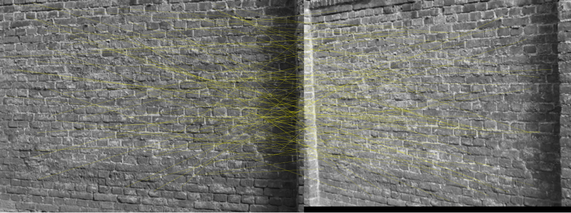
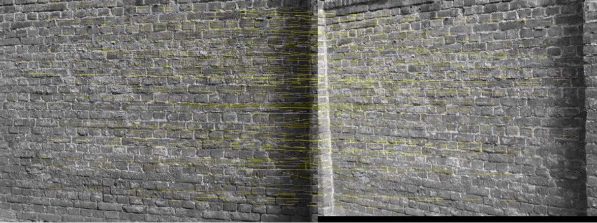
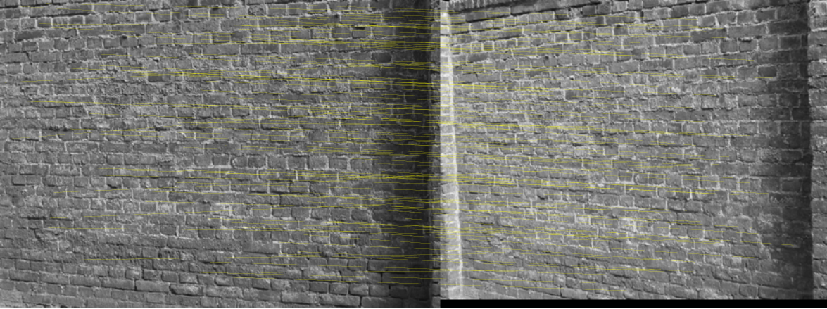
In this set of experiments, weighted graphs were constructed from the CMU House sequence images11 1 http://vasc.ri.cmu.edu/idb/html/motion/, which has been wildly used for testing graph matching algorithms. In the previous literature, only small graphs (30 nodes) were extracted from the images for matching. To demonstrate scalability of FastPFP, we applied SIFT feature descriptor [42] to all CMU House sequence images. Roughly 800 keypoints were extracted for each image and the number of keypoints varies from image to image. All keypoints in an image were used for the construction of a graph. For each image, a graph whose nodes represent keypoints and edges (matrix ) represent Euclidean distance between keypoints in that image was constructed. For a visualization, we show in Fig. 3 feature correspondence for image 0 vs. image 110. Results of PG, FastGA and FastPFP were shown.
We matched the first image and subsequent images, i.e. image vs. image 1, image 0 vs. image 2, …, and image 0 vs. image 110. The runtime and matching error (measured as ) were recorded for different algorithms. The results are shown in Fig. 4. FastPFP is about 6 times faster than FastGA, with even much lower matching error.
V-C Graphs From Real Images
In this set of experiments, attributed and weighted graphs were constructed from real images, chosen from the four image sets: Graffiti, Wall, Bark and Boat22 2 http://www.robots.ox.ac.uk/~vgg/research/affine/. The graphs were constructed as follows. We first applied SIFT descriptor to extract 128-dimensional features for each image. Then a simple feature selection was performed as follows: a feature of an image was selected if it has the similarity (inner product) to all features of its counterpart image above a threshold. From the selected features, a graph was constructed. Each node represents a keypoint, each node attribute represents a SIFT 128-dimensional feature vector, and each edge represents the Euclidean distance between nodes. Each element of is set to be the inner product of two SIFT feature vectors and . See Fig. 6 for visualization of the matching results for PG, FastGA and FastPFP. The experimental results are listed in Table III and III. The runtime and matching error (measured as ) were recorded. is used. The sensitivity study of parameter is given in Section VI-B. Again, FastPFP demonstrated the best performance: it is about times faster than FastGA while usually achieving a much lower matching error.
| Graph pair | PG | FastGA | FastPFP |
|---|---|---|---|
| Graffiti | 51.60 | 87.89 | |
| Wall | 19.94 | 32.25 | |
| Bark | 2.84 | 2.72 | |
| Boat | 5.59 | 9.06 |
| Graph pair | PG | FastGA | FastPFP |
|---|---|---|---|
| Graffiti | 2.75 | 3.98 | |
| Wall | 1.31 | 1.01 | |
| Bark | 3.07 | ||
| Boat | 4.77 | 3.18 |
V-D Graphs From 3D Points
In this set of experments, weighted graphs were constructed from 3D points. The Face 50 and Stanford Bunny 3D points datasets33 3 Both datasets can be downloaded in https://sites.google.com/site/myronenko/ were used. In the Face 50 dataset, each face has 392 points, all of which were used for the construction of graphs. In the Stanford Bunny 3D data, each set of 3D points was downsampled to 1022 points. Graphs, whose edge represents Euclidean distance between two points, were constructed. The visualization of matching results of PG, FastGA, FastPFP and Umeyama’s method are shown in Fig. 7 and 8. The matching error (measured as ) and runtime are shown in Table V and V. Again, FastPFP outperformed the others in both speed and accuracy. FastPFP is about 15 20 times faster than FastGA.
| Graph pair | PG | FastGA | Umeyama | FastPFP |
|---|---|---|---|---|
| Face pair 1 | 2.90 | 15.05 | 18.40 | |
| Face pair 2 | 3.06 | 15.53 | 18.23 | |
| Stanford Bunny | 21.74 | 118.55 | 1027.02 |
| Graph pair | PG | FastGA | Umeyama | FastPFP |
|---|---|---|---|---|
| Face pair 1 | 6.30 | 14.3 | 12.5 | |
| Face pair 2 | 6.23 | 16.2 | 10.6 | |
| Stanford Bunny | 29.1 | 37.4 | 32.7 |
VI Discussion
VI-A Comparison To FastGA
Although FastGA and FastPFP both have time complexity per iteration, FastPFP is empirically about times faster than FastGA. This is mainly due to the slow convergence of FastGA. Despite the theoretical work on convergence of FastGA [35], empirically FastGA does not have good convergence speed, as observed in the experiments. To see that, we show the magnitude of parameter for image sequence (image 0 vs. image 110) and real image (Graffiti) for 20 iterations in Fig. 9. Besides good convergence, FastPFP only requires simple arithmetic operations (addition, multiplication and maximum element search) while FastGA requires additionally exponentiation and logarithm (for numerically stable implementation).
VI-B Parameter Sensitivity

The performance of FastPFP is not very sensitive to the step size parameter , for . In Fig. 10, the runtime and matching error of FastPFP in the image sequence (image 0 vs. image 110) and the real image experiment (Graffiti) are shown for different values of , ranging from 0.1 to 1. The performance of FastPFP is unstable for .
For attributed graph matching, the matching quality is not very sensitive to the parameter . We show the matching result for (which means the matching objective function becomes and is solved by Hungarian method), and . The results are similar except for . The matching results are shown in Fig. 11.
VI-C Limitations
Despite the encouraging experimental results, our algorithm is derived heuristically, as many other approximate graph matching algorithms such as GA (FastGA), Umeyama’s method, SM and RWRW. For these algorithms including ours, the optimality of the solutions is not theoretically guaranteed. Also, our algorithm does not use an edge compatibility matrix, due to its high computational cost. Consequently, another limitation of our algorithm is its inability to handle arbitrary edge relationship (some graphs have vector edge attributes), unlike those algorithms based an edge compatibility matrix.
VII Conclusion
We proposed a new fast graph matching algorithm based on a new projected fixed-point method, suitable for large graph matching. Extensive experiments were conducted to demonstrate the strength of our algorithm over previous state-of-the-art algorithms. Future work includes theoretical analysis, extension and applications of our algorithm.
Acknowledgements
References
- [1] D. Conte, P. Foggia, C. Sansone, and M. Vento, ”Thirty Years of Graph Matching in Pattern Recognition,” Int’l J. of Pattern Recognition and Aritificial Intelligence, vol. 18, no. 3, pp. 265-298, 2004.
- [2] H. Bunke and B.T. Messmer, ”Recent Advances in Graph Matching,” IEEE Trans. Pattern Analysis and Machine Intelligence, vol. 11, pp. 169-203, 1997.
- [3] R.S.T. Lee and J.N.K. Liu, ”An Oscillatory Elastic Graph Matching Model for Recognition of Offline Handwritten Chinese Characters,” Proc. Third Int’l Conf. Knowledge-Based Intelligent Information Eng. Systems, pp. 284-287, 1999.
- [4] A. Filatov, A. Gitis, and I. Kil, ”Graph-Based Handwritten Digit String Recognition,” Proc. Third Int’l Conf. Document Analysis and Recognition, pp. 845-848, 1995.
- [5] S. Belongie, J. Malik, and J. Puzicha, ”Shape Matching and Object Recognition Using Shape Contexts,” IEEE Trans. Pattern Analysis and Machine Intelligence, vol. 24, no. 4, pp. 509-522, Apr. 2002.
- [6] A.C. Berg, T.L. Berg, and J. Malik, ”Shape Matching and Object Recognition Using Low Distortion Correspondences,” IEEE Int’l Conf. Computer Vision and Pattern Recognition, vol. 1, pp. 26-33, 2005.
- [7] K. Siddiqi, A. Shokoufandeh, S.J. Dickinson, and S.W. Zucker, ”Shock Graphs and Shape Matching,” Int’l J. Computer Vision, vol. 35, no. 1, pp. 13-32, 1999.
- [8] B. Huet and E.R. Hancock, ”Shape Recognition From Large Image Libraries by Inexact Graph Matching,” Pattern Recognition Letters, vol. 20, no. 11-13, pp. 1259-1269, Nov. 1999.
- [9] L. Wiskott, J.M. Fellous, N. Krüer, and C. von der Malsburg, ”Face Recognition by Elastic Bunch Graph Matching,” IEEE Trans. Pattern Analysis and Machine Intelligence, vol. 19, no. 7, pp. 775-779, July 1997.
- [10] L. Torresani, V. Kolmogorov, and C. Rother, ”Feature Correspondence via Graph Matching: Models and Global Optimization,” Proc. European Conf. on Computer Vision, pp. 596-609, 2008.
- [11] Y. Zheng and D. Doermann, ”Robust Point Matching for Nonrigid Shapes by Preserving Local Neighborhood Structures,” IEEE Trans. Pattern Analysis and Machine Intelligence, vol. 28, no. 4, pp. 643-649, April 2006.
- [12] S. Berretti, A.D. Bimbo, and E. Vicario, ”Efficient Matching and Indexing of Graph Models in Content-Based Retrieval,” IEEE Trans. Pattern Analysis and Machine Intelligence, vol. 23, no. 10, pp. 1089-1105, Oct. 2001.
- [13] K. Shearer, H. Bunke, and S. Venkatesh, ”Video indexing and similarity retrieval by largest common subgraph detection using decision trees,” Pattern Recognition, vol 34, no. 5, pp. 1075-1091, May 2001.
- [14] J.R. Ullman, ”An Algorithm for Subgraph Isomorphism,” J. ACM, vol. 23, no. 1, pp. 31-42, Jan. 1976.
- [15] B.D. McKay, ”Practical Graph Isomorphism,” Congressus Numerantium, vol. 30, pp. 45-87, 1981.
- [16] L.P. Cordella, P. Foggia, C. Sansone, and M. Vento, ”A (Sub)Graph Isomorphism Algorithm for Matching Large Graphs,” IEEE Trans. Pattern Analysis and Machine Intelligence, vol. 26, no. 10, pp. 1367-1372, Oct. 2004.
- [17] W.H. Tsai and K.S. Fu, ”Error-Correcting Isomorphisms of Attributed Relational Graphs for Pattern Analysis,” IEEE Trans. Systems, Man, and Cybernetics, vol. 9, no. 12 pp. 757-768, Dec. 1979.
- [18] L.G. Shapiro and R.M. Haralick, ”Structural Descriptions and Inexact Matching,” IEEE Trans. Pattern Analysis and Machine Intelligence, vol. 3, no. 5 pp. 504-519, Sept. 1981.
- [19] M.A. Fischler and R.A. Elschlager, ”The Representation and Matching of Pictorial Structures,” IEEE Trans. Computers vol. 22 no. 1, Jan. 1973.
- [20] A. Rosenfeld, R.A. Hummel, and S.W. Zucker, ”Scene Labeling by Relaxation Operations,” IEEE Trans. Systems, Man, and Cybernetics, vol. 6, no. 6, pp. 420-433, 1976.
- [21] R.A. Hummel and S.W. Zucker, ”On The Foundations of Relaxation Labeling Procesesses,” IEEE Trans. Pattern Analysis and Machine Intelligence, vol. 5, no. 3, pp. 267-286, 1983.
- [22] W.J. Christmas, J. Kittler, and M. Petrou, ”Structural Matching in Computer Vision Using Probabilistic Relaxation,” IEEE Trans. Pattern Analysis and Machine Intelligence, vol. 17, no. 8, pp. 749-764, Aug. 1995.
- [23] S. Gold and A. Rangarajan, ”A Graduated Assignment Algorithm for Graph Matching,” IEEE Trans. Pattern Analysis and Machine Intelligence, vol. 18, no. 4, pp. 377-388, Apr. 1996.
- [24] H. Almohamad and S. Duffuaa, ”A Linear Programming Approach for the Weighted Graph Matching Problem,” IEEE Trans. Pattern Analysis and Machine Intelligence, vol. 15, no. 5, pp. 522-525, May 1993.
- [25] B.J. van Wyk and M.A. van Wyk, ”A POCS-Based Graph Matching Algorithm,” IEEE Trans. Pattern Analysis and Machine Intelligence, vol. 26, no. 11, Nov. 2004.
- [26] M. Leordeanu and M. Hebert, ”A Spectral Technique for Correspondence Problems Using Pairwise Constraints,” Proc. Int’l Conf. Computer Vision, 2005.
- [27] T. Cour, P. Srinivasan, and J. Shi, ”Balanced Graph Matching,” Proc. Advances in Neural Information Processing Systems, pp. 313-320, 2006.
- [28] R. Zass and A. Shashua, ”Probabilistic Graph and Hypergraph Matching,” IEEE Int’l Conf. on Computer Vision and Pattern Recognition, pp. 1-8, 2008.
- [29] M. Leordeanu, M. Hebert, and R. Sukthankar, ”An Integer Projected Fixed Point Method for Graph Matching and MAP Inference,” Proc. Advances in Neural Information Processing Systems, pp. 1114-1122, 2009.
- [30] M. Cho, J. Lee, and K.M. Lee, ”Reweighted Random Walks for Graph Matching,” Proc. European Conf. on Computer Vision, pp. 492-505, 2010.
- [31] M. Zaslavskiy, F. Bach, and J.P. Vert, ”A Path Following Algorithm for the Graph Matching Problem,” IEEE Trans. Pattern Analysis and Machine Intelligence, vol. 31, no. 12, pp. 2227-2242, Dec. 2009.
- [32] H.W. Kuhn, ”The Hungarian Method for the Assignment Problem,” Naval Research Logistics Quarterly, vol. 2, nos. 1/2, pp. 83-97, 1955.
- [33] S. Umeyama, ”An Eigendecomposition Approach to Weighted Graph Matching Problems,” IEEE Trans. Pattern Analysis and Machine Intelligence, vol. 10, no. 5, pp. 695-703, Sept. 1988.
- [34] P.H. Calamai, ”Projected Gradient Methods for Linearly Constrained Problems,” Mathematical Programming, vol. 39, no. 1, Oct. 1987.
- [35] A. Rangarajan, A. Yuille, and E. Mjolsness, ”Convergence Properties of the Sofassign Quadratic Assignment Algorithm,” Neural Computation, vol. 11, pp. 1455-1474, 1999.
- [36] R.E. Burkard, E. Cela, P.M. Pardalos, and L.S. Pitsoulis, ”The Quadratic assignment problem,” Handbook of Combinatorial Optimization, 1998.
- [37] E.H, Zarantonello, ”Projections on Convex Sets in Hilbert Space and Spectral Theory,” Contributions to Nonlinear Functional Analysis, pp. 237-424, Academic Press, New York, 1971.
- [38] D.C. Youla and H. Webb, ”Image Restoration by the Method of Convex Projections: Part 1 - Theory,” IEEE Trans. Medical Imaging, vol. 1, no. 2, Oct. 1982.
- [39] R. Sinkhorn, ”A Relationship between Arbitrary Positive Matrices and Doubly Stochastic Matrices,” Annals Math. and Statistics, vol. 35, pp. 876-879, 1964.
- [40] R. Zass and A. Shashua, ”Doubly Stochastic Normalization for Spectral Clustering,” Proc. Advances in Neural Information Processing Systems, 2007.
- [41] J. Von Neumann, Functional Operators, vol. II. Princeton University Press, 1950.
- [42] D.G. Lowe, ”Distinctive Image Features from Scale-Invariant Keypoints,” Int’l J. of Computer Vision, vol. 60, no. 2, Nov. 2004.
Appendix
FastGA
In general, GA also has time complexity per iteration. However, when the compatibility matrix (which was mentioned in the original paper of GA [23]) is used, GA has only time complexity per iteration. To see this, consider the most time-consuming step of GA, which has time complexity
| (34) |
where is the soft-assignment matrix. If , then (34) can be compactly written as
| (35) |
which has time complexity .
Problem Formulation
Successive Projection
The derivation of (23)(24) is due to [40], with slight modification in here. We first consider . The Lagrangian of (21) is
| (43) | ||||
| (44) |
Let and set the derivative with respect to to zero, we have
| (45) |
Multiplies by 1 on both sides: . Combining the fact that , we obtain (23). The derivation of (24) is straightforward and omitted.
| Yao Lu |
| Kaizhu Huang |
| Cheng-Lin Liu |