•

c.o.m.: Center of mass.
•

CL: Confidence level.
•

EW: Electroweak.
•

FB: Forward-backward.
•

GB: Goldstone boson.
•

LH: Little Higgs.
•

LHC: Large Hadron Collider.
•

LO: Leading order.
•

MSSM: Minimal Supersymmetric Standard Model.
•

NLO: Next to leading order.
•

PDF: Parton distribution function.
•

SM: Standard Model.
•

SUSY: Supersymmetry.
•

VEV: Vacuum expectation value.

Introduction

The Standard Model (SM) of particle physics, one of the greatest achievements of the 20th century, has proved to be an extraordinarily successful theory to describe the physics at colliders below the TeV scale. However, one of the most important pieces of the theory, the mechanism responsible for the electroweak (EW) symmetry breaking, has not been confirmed yet. The main objective of the Large Hadron Collider (LHC) at CERN is to reveal the nature of this mechanism, i.e., the search for the Higgs boson, the measure of its mass and couplings. The discovery of the Higgs and of possible new particles and symmetries related to the Higgs mechanism will define a new theoretical framework valid at energies above the TeV scale.

The LHC was inaugurated in 2008 and, after solving a few problems with the set-up, in 2010 it became the most powerful collider in the world, beating the Fermilab Tevatron. Data from its experiments ATLAS and CMS suggest the existence of a Higgs boson of 125 GeV compatible with the one predicted by the SM. Although we are still waiting for experimental confirmation from the data collected during 2012, the mass range where it could be found is already very constrained. We are certainly living an exciting time in particle physics.

In addition, so far LHC data do not seem to indicate any new physics beyond the SM. As a consequence, neutrino masses and the existence of dark matter are the only experimental evidences currently indicating that the model must be completed. Of course, there is the formal argument known as the hierarchy problem, which has been the main motivation for model building during the past 30 years and that the LHC should definitively solve. Although not at the level of discovery, there are also experimental anomalies that motivate phenomenological studies of different extensions of the SM. In particular, during the preparation of this Thesis one of these anomalies has achieved special relevance, the forward-backward asymmetry in $t\bar{t}$ production measured at the last stage of the Tevatron. This unexpected effect attracted the attention of the particle physics community (there are over 100 articles appeared during 2011), and it became also my main research line during the past year. But this is the end of the story; let us start from the beginning.

When we planned my Ph.D. project in 2008, we decided that in a first phase we would analyze different extensions of the SM such as Little Higgs, Supersymmetry and Extra Dimensions. In a second stage and after the initial results from the LHC, we would focus on the phenomenology of the model that were favored by the data. However, due both to the delay in the LHC set-up and to the fact that the first observations pointed nowhere besides the SM, I had to slightly rethink the final destination of this Thesis. Thus, in this work two different parts can be distinguished. In the first one I describe some scenarios for new physics and discuss our contributions in each of them. In the second part I focus on the experimental hint of new physics that I consider most interesting, the forward-backward asymmetry in $t\bar{t}$ production measured at the Tevatron, analyzing in detail its possible implications at the LHC.

As it is mandatory in any Ph.D. Thesis in particle physics, I start reviewing the SM. I pay special attention to the Higgs sector and to the main motivation for this Thesis: the hierarchy problem and the need for new physics. Theoretical and experimental constraints on the Higgs boson mass are also discussed.

The second chapter is focused on Little Higgs models, in particular, on the so-called simplest model. After a short review I discuss our main contribution, the possibility that the model accommodates in a consistent way a vectorlike $T$ quark relatively light, of mass around 500 GeV. We show that this is possible by slightly changing the collective symmetry breaking principle in the original model for an approximate breaking principle. We find the anomalous couplings of the top quark and the Higgs boson in that scenario, and we deduce the one-loop effective potential, showing that it implies an EW symmetry breaking and a scalar mass spectrum compatible with the data.

The third chapter is dedicated to the phenomenological implications that new Higgs bosons could have in $t\bar{t}$ production. We study the possible effects caused by the massive scalars present in supersymmetric and Little Higgs models. After a review of the Higgs sector in supersymmetric models, we analyze the effect of these scalars on $t\bar{t}$ when they are produced in the s-channel of gluon fusion. We first study the cross sections at the parton level and then we analyze $pp$ collisions at the LHC.

The last chapter is devoted to the forward-backward asymmetry in $t\bar{t}$ production. I start reviewing the observations and their compatibility with the SM. Then I discuss the effects of a generic massive gluon on that observable. We propose a framework with a gluon of mass below 1 TeV, with small and mostly axial-vector couplings to the light quarks and large coupling to the right-handed top quark. The key ingredient to define our stealth gluon, invisible in other observables, is a very large decay width caused by new decay channels $qQ$ , where $q$ is a standard quark and $Q$ a massive excitation with the same flavor. The model requires the implementation of energy-dependent widths, something that is not common in previous literature. We check that the model reproduces both the asymmetry and the $t\bar{t}$ invariant-mass distribution at hadron colliders, and we study the phenomenological implications of the quarks $Q$ . We study how the new $qQ$ channel affects current analyses of $t\bar{t}$ production and of $T\bar{T}$ searches at the LHC. We also discuss the best strategy to detect the $qQ$ channel at that collider. We have included three appendixes with details about the event selection and reconstruction, which are along the lines of those used by the different LHC experiments.

The results contained in this Thesis have led to several publications. The study of the Little Higgs models produced two publications [2, 3], the first one done during a research fellowship awarded in the last year of my undergraduate studies. During the year 2009 we also published a work [4] on models with extra dimensions, another scenario proposed to solve the hierarchy problem. In particular, we studied the interaction of cosmic rays with galactic dark matter in models with strong gravity at the TeV scale. Since this work, unlike the rest, does not involve collider physics, I decided not to include it in this Thesis. The results about $t\bar{t}$ production through new Higgs bosons gave one publication [5]. Finally, our results on the forward-backward asymmetry in $t\bar{t}$ production and the study of new massive quarks at the LHC in Chapter 4 have appeared in three publications [6, 7, 8].

In addition, I had the opportunity to make a presentation in the conference $2^{\textrm{nd}}$ Young Researchers Workshop: Physics Challenges in the LHC Era in Frascati (Italy), May of 2010 [9]. I made presentations in the Bienal de Física Española in 2009 and 2011. I could also discuss these results in a Seminar at the University of Oxford (July 2011), where I was visiting during three months.

Chapter 1 The Standard Model and beyond

Although the Standard Model (SM) of particle physics can not be considered as a complete theory of fundamental interactions, due to its success in explaining a wide variety of experiments it is sometimes regarded as a theory of ‘almost’ everything. The SM summarizes our understanding of the microscopic world and, in this sense, it is the result of a long story that involves the efforts of many people. In the 19th century John Dalton, through his work on stoichiometry, concluded that each given element of nature was composed of a single type of extremely small object. He believed that these objects were the elementary constituents of matter and named them atoms, after the Greek word $\alpha\tau o\mu o$ , meaning ‘indivisible’. Near the end of that century J.J. Thompson showed that, in fact, atoms were not the fundamental objects of nature but that they had structure and are conglomerates of even smaller particles. Early 20th-century explorations (Fermi, Hahn, Meitner) culminated in proofs of nuclear fission, a discovery that gave rise to an active industry of generating one atom from another. Throughout the 1950s and 1960s, the first accelerators revealed a bewildering variety of particles that could be produced in scattering experiments. With all these data, in 1961 Sheldon Glashow [10] proposed a model combining the electromagnetic and the weak interactions which was completed in 1967 by Steven Weinberg [11] and, independently in 1968, by Abdus Salam [12]. Together with Quantum Chromodinamics (QCD) for the description of the strong interactions, it defines what is called the SM of particle physics. An important ingredient of this theory was proposed in 1964 by Peter Higgs [13], and it has still to be fully confirmed at the LHC Collider.

In this chapter we will briefly review the SM, paying special attention to the Higgs sector: present bounds on the Higgs mass, the hierarchy problem, and the need for physics beyond the SM. Good reviews about the SM (and beyond) are [14, 15, 16, 17, 18, 19, 20, 21, 22].

1.1 The Standard Model

The SM is a renormalizable relativistic quantum field theory describing three of the four fundamental interactions observed in nature: electromagnetic, weak and strong interactions. This description is based on a local gauge symmetry $SU(3)_{C}\times SU(2)_{L}\times U(1)_{Y}$ spontaneously broken to $SU(3)_{C}\times U(1)_{EM}$ . The fourth fundamental interaction, gravity, is outside this framework. In this sense, the SM could be considered an effective theory only valid at energies below the Planck scale, where gravitational interactions between elementary particles would be unsuppressed.

The gauge principle describes the SM interactions in terms of one spin-1 massless boson per each unbroken symmetry: 8 gluons ( $g$ ) corresponding to the strong interactions and 1 photon ( $\gamma$ ) for the electromagnetism. In addition, the 3 broken symmetries imply the presence of 3 massive bosons ( $W^{\pm}$ and $Z$ ) as mediators of the weak interactions.

The fermionic matter should be accommodated in multiplets (irreducible representations) of the group transformations. The number of copies (or families) of different mass is not fixed by the gauge symmetry, being minimality and the absence of quantum anomalies the guiding principles. The SM includes three families of quarks (triplets under $SU(3)_{C}$ ) and three of leptons (color singlets). All these particles are chiral under the SM symmetry: the left-handed components define doublets under $SU(2)_{L}$ , while the right-handed components are singlets. Therefore, they only get masses after the electroweak (EW) symmetry is broken. Each lepton family consists of a neutrino ( $\nu_{l}$ ) and a charged lepton ( $l^{-}$ ) and for the quarks, each family contains an up ( $u$ ) and a down ( $d$ ) type quark of electric charge $+2/3$ and $-1/3$ , respectively, plus the corresponding antiparticles. A (vectorlike) right-handed neutrino is not necessary, so it is not included (see Table. 1.1). The electric charge ( $Q$ ), the isospin ( $T_{3}$ ) and the hypercharge ( $Y$ ) are related by the expression $Q=T_{3}+Y$ [13, 23, 24, 25].

Multiplets

\mathbf{SU(3)_{c}\times SU(2)_{L}\times U(1)_{Y}}

III

Quarks

(3,2,

-\frac{1}{6}

)

\left(\begin{array}[]{c}u_{L}\\ d_{L}\\ \end{array}\right)

\left(\begin{array}[]{c}c_{L}\\ s_{L}\\ \end{array}\right)

\left(\begin{array}[]{c}t_{L}\\ b_{L}\\ \end{array}\right)

s=1/2

(3,1,

\frac{2}{3}

)

u_{R}

c_{R}

t_{R}

(3,1,

-\frac{1}{3}

)

d_{R}

s_{R}

b_{R}

Leptons

(1,2,

-\frac{1}{2}

)

\left(\begin{array}[]{c}{\nu_{e}}_{L}\\ e_{L}\\ \end{array}\right)

\left(\begin{array}[]{c}{\nu_{\mu}}_{L}\\ \mu_{L}\\ \end{array}\right)

\left(\begin{array}[]{c}{\nu_{\tau}}_{L}\\ \tau_{L}\\ \end{array}\right)

s=1/2

(1,1,

-1

)

e_{R}

\mu_{R}

\tau_{R}

Higgs

s=0

(1,2,

\frac{1}{2}

)

H=\left(\begin{array}[]{c}h^{+}\\ h^{0}\end{array}\right)

Table 1.1: Field multiplets in the SM.

An important aspect, sometimes taken as a measure of its elegance, is the number of free parameters in the SM. It has 18 free parameters: 9 fermion masses, 3 CKM mixing angles plus 1 phase, 3 gauge couplings, and 2 parameters (the vacuum expectation value of the Higgs field and its physical mass) in the scalar sector. The $CP$ -violating $\theta$ angle of QCD can be considered the 19th free parameter of the SM, but it is constrained experimentally to be very close to zero. Finally, neutrino masses can be obtained through dimension-5 operators and/or adding right-handed neutrinos, and will define another 7 or 9 new free parameters. However, strictly speaking they are not part of the SM but physics beyond it.

1.2 The Higgs mechanism in the SM

The Higgs mechanism is a process by which gauge bosons can get a mass. It was first proposed in 1962 by Anderson [26], who discussed its consequences for particle physics but did not work out an explicit relativistic model. Such a model was developed in 1964 by Higgs [13] and, independently, by Brout & Englert [23] and Guralnik, Hagen & Kibble [24]. The mechanism is closely analogous to phenomena previously discovered by Nambu involving the vacuum structure of quantum fields in superconductivity [27].

In the SM, the addition by hand of vector-boson and fermion masses leads to a manifest breakdown of the local $SU(2)_{L}\times U(1)_{Y}$ gauge invariance. The Higgs mechanism, instead, assumes that the symmetry is broken spontaneously: while the theory (the Lagrangian) is $SU(2)_{L}\times U(1)_{Y}$ invariant, the vacuum (the field configuration with minimum energy) is not, it breaks the symmetry to $U(1)_{EM}$ . As a consequence, the $W^{\pm}$ and $Z$ gauge bosons and all the matter fields will acquire masses through interactions with the vacuum. From a formal point of view, such procedure will preserve the gauge principle and, most important, will keep all the properties (renormalizability, unitarity) that make gauge theories consistent. From a phenomenological point of view, it will imply a relation between the $Z$ and $W$ masses and will explain that the photon is massless and the electric charge conserved.

Let us see more explicitly how this happens. We need to introduce a scalar field with, at least, 3 degrees of freedom. The simplest choice is a complex $SU(2)$ doublet,

\Phi=\left(\begin{array}[]{c}\phi^{+}\\ \phi^{0}\end{array}\right)_{Y=+{1\over 2}}\;.

(1.1)

Imposed gauge invariance and renormalizability its Lagrangian reads

\mathcal{L_{S}}=(D^{\mu}\Phi)^{\dagger}(D_{\mu}\Phi)-V(\Phi)\,,

(1.2)

with

V(\Phi)=\mu^{2}\Phi^{\dagger}\Phi+\lambda(\Phi^{\dagger}\Phi)^{2}\,.

(1.3)

If the mass parameter $\mu^{2}$ is positive ( $\lambda$ must be positive as well to make the potential bounded from below) then $\mathcal{L}_{S}$ is simply the Lagrangian of 4 spin-zero particles ( $\Phi^{\pm}$ , $\Phi^{0}$ and $\bar{\Phi}^{0}$ ) of equal mass $\mu$ .

Refer to caption — Figure 1.1: Projection in the plane $\phi^{+}$ = 0 of the potential V( $\Phi$ ) in the cases $\mu^{2}>0$ (left) and (‘Mexican hat’) $\mu^{2}<0$ (right).

However, if $\mu^{2}<0$ the origin becomes unstable and the minimum of the effective potential will define a vacuum expectation value (VEV)

|\langle\Phi\rangle|={1\over\sqrt{2}}v\,,

(1.4)

with $v=\sqrt{-\mu^{2}/\lambda}$ at the tree level. Although the minimum is degenerated, all the minima are equivalent (related by the gauge symmetry), and with all generality we can take the real component of the neutral component as the only one developing a non-zero VEV,

\langle\Phi\rangle_{0}\equiv\langle 0|\Phi|0\rangle={1\over\sqrt{2}}\left(\begin{array}[]{c}0\\ v\end{array}\right)\,.

(1.5)

With this choice the vacuum is neutral under $Q=T_{3}+Y$ , which generates the unbroken $U(1)_{EM}$ , whereas the rest of the $SU(2)_{L}\times U(1)_{Y}$ symmetry is spontaneously broken. The scalar excitations along the flat directions of the potential will then define three Goldstone bosons $\theta_{i}$ [28, 29]. We may parametrize the scalar doublet as

\Phi={1\over\sqrt{2}}\exp{\left(i\theta_{i}(x){\sigma_{i}\over 2}\right)}\left(\begin{array}[]{c}0\\ v+h(x)\end{array}\right),

(1.6)

being $\theta_{i}(x)$ and $h(x)$ real fields and $\sigma_{i=1,2,3.}$ the Pauli matrices. Now, we can move to the so-called unitary gauge by rotating away the three Goldstone bosons, that are ‘eaten’ by the $W^{\pm}$ and $Z$ bosons:

\Phi(x)\rightarrow\Phi(x)={1\over\sqrt{2}}\left(\begin{array}[]{c}0\\ v+h(x)\end{array}\right).

(1.7)

Operating algebraically in the Lagrangian we see that the $W$ and $Z$ bosons get masses while the photon remains massless,

M_{W}={1\over 2}vg,\;M_{Z}={1\over 2}v\sqrt{g^{2}+g^{\prime 2}},\;M_{\gamma}=0\,,

(1.8)

where $g$ and $g^{\prime}$ are the $SU(2)_{L}$ and $U(1)_{Y}$ coupling constants, respectively.

Let us see now how the fermions become massive. We will use their Yukawa interactions with the Higgs doublet $\Phi$ and its conjugate $\tilde{\Phi}=i\sigma_{2}\Phi^{*}$ , with hypercharge $Y=-{1\over 2}$ (it transforms the same way as $\Phi$ under $SU(2)_{L}$ ). For one fermion generation we obtain gauge invariant interactions combining the left-handed doublets with the right-handed singlets and the Higgs doublet,

\mathcal{L_{\textrm{Yukawa}}}=-y_{e}\bar{L}\Phi e_{R}-y_{u}\bar{Q}\tilde{\Phi}u_{R}-y_{d}\bar{Q}\Phi d_{R}+h.c.\;.

(1.9)

After the Higgs VEV we obtain

m_{e}={y_{e}v\over\sqrt{2}},\;m_{u}={y_{u}v\over\sqrt{2}},\;m_{d}={y_{d}v\over\sqrt{2}}.

(1.10)

For three generations $y_{e,u,d}$ must be replaced by $3\times 3$ matrices of Yukawa couplings.

Since the Higgs couples to gauge bosons and fermions proportional to their masses, it will decay into the heaviest ones accessible at the phase space. In Fig. 1.2 we show its decay branching ratios as a function of its mass.

1.3 The Higgs particle in the SM

In the unitary gauge there is only one degree of freedom, $h$ , which corresponds to the physical Higgs boson. Its kinetic term and gauge interactions come from the covariant derivative $|D_{\mu}\Phi|^{2}$ , while its mass and self-interactions derive from the scalar potential. In particular, in terms of the couplings in Eq. (1.3) one has

m_{h}^{2}=2\lambda v^{2}=-2\mu^{2},

(1.11)

with the VEV $v=246$ GeV in order to reproduce the $W$ boson mass. In the SM a measurement of $m_{h}$ would also fix all its self-interactions.

Although the mass of the SM Higgs is still unknown, there are interesting theoretical constraints that can be derived from assumptions on the energy range in which the SM is valid before perturbation theory breaks down and new phenomena emerge. These include constraints from unitarity in scattering amplitudes, perturbativity of the Higgs self-coupling and stability of the EW vacuum. In particular, unitarity constraints in longitudinally polarized $WW$ scattering imply that the Higgs mass should not be much larger than 1 TeV¹¹ 1 A similar argument was the basis to abandon the old Fermi theory for the weak interaction.. Triviality limits are derived assuming the SM to be valid up to some energy scale and requiring that the self-coupling of the Higgs field does not blow up in the running. For a value of the cut-off scale not much larger than $m_{h}$ this implies that $m_{h}\lesssim 800$ GeV, while $m_{h}\lesssim 150$ GeV if we assume perturbativity up to the reduced Planck scale ( $\sim 10^{18}$ GeV). Theoretical considerations about the stability of the scalar potential under top-quark corrections to $\lambda$ provide lower bounds on $m_{h}$ , also depending on the cut-off scale of the SM. If, again, we assume the SM is valid up to the reduced Planck scale, vacuum stability requires $m_{h}\gtrsim 130$ GeV, and $m_{h}\gtrsim 115$ GeV if we simply require a sufficiently long-lived metastable vacuum.

Later we will discuss the different experimental constraints on $m_{h}$ coming from direct and indirect searches, but before we would like to review the main reason to expect physics beyond the SM associated to the Higgs boson.

1.4 The hierarchy problem

Despite the extraordinary strength of the SM from an experimental point of view, it has been emphasized during the past 30 years the need for additional physics that provides formal consistency to its Higgs sector and solves the so-called hierarchy problem. If we assume the SM valid up to an energy scale $\Lambda$ (its cut-off) then the Higgs mass parameter ( $\mu^{2}$ ) receives one-loop corrections that grow proportional to $\Lambda^{2}$ . The three most significant quadratic contributions come from one-loop diagrams with the top quark, the gauge bosons and Higgs self-interactions:

\Delta\mu^{2}=-\frac{3}{8\pi^{2}}y_{t}^{2}\Lambda^{2}+{9\over 64\pi^{2}}g^{2}\Lambda^{2}+{1\over 16\pi^{2}}\lambda\Lambda^{2}\,.

(1.12)

The Higgs mass parameter in the effective potential includes then one-loop plus (arbitrary) tree-level contributions. If the SM is all the physics that there is between the EW and the Planck or the Grand Unification scale (i.e., $\Lambda\thicksim 10^{19}\textrm{ GeV}$ or $\Lambda\thicksim 10^{16}\textrm{ GeV}$ ), these different contributions should cancel around 30 digits to get the observed value of order $v^{2}$ ( $\mu^{2}=-v^{2}\lambda\thicksim-(100\textrm{ GeV})^{2}$ ). Moreover, this cancellation must take place at every order in perturbation theory, since another quadratic divergence appears at two-loops and so on. This fine tuning is considered unnatural and suggests that the scale $\Lambda$ for new physics (new symmetries or dynamics) that explains the cancellation is not very high.

To get one-loop corrections to $\mu^{2}$ smaller than 10 times its total value (i.e., less than 10% of fine tuning) the cut-off in each sector should satisfy

\Lambda_{top}<2\textrm{ TeV,}\qquad\Lambda_{gauge}<5\textrm{ TeV,}\qquad\Lambda_{Higgs}<12\textrm{ TeV.}

(1.13)

Therefore, one could expect that below those energies the new physics becomes effective and defines a corrected SM free of quadratic corrections to $\mu^{2}$ . In this way, the new physics is most needed to cancel the top-quark contribution, which favors the existence of new top-like particles (related to the top quark by symmetries) or a special (composite) nature for this quark observable below this threshold. In addition, one also expects that the new physics should couple to the Higgs as strongly as the top quark, so the Higgs search at hadron colliders could be very correlated with the search for new top-quark physics. In a similar way, we would expect the extra physics canceling gauge-boson corrections below 5 TeV, which suggests a less relevant role at the LHC but that could conflict the data on precision EW observables. Finally, Higgs self-interactions require new physics below 12 TeV for $m_{h}=125$ GeV.

As the center of mass (c.o.m.) energy at the LHC may reach 14 TeV, these are compelling arguments to explore there the different possibilities for the so-called physics beyond the Standard Model. If the hierarchy problem is to be solved by new physics, we should see it at the LHC. Some frameworks for this physics to be analyzed in later chapters are:

•

Supersymmetry (SUSY), probably the favorite candidate of the community over the past 30 years. There is the increasing feeling, however, that it should have already given any experimental signal, specially in precision experiments (electric dipole moments, flavor physics). The discovery of a light Higgs could provide renewed interest. We will discuss the SUSY Higgs sector in Chapter 3.
•

Models where the Higgs is a pseudo-Goldstone boson of a global symmetry broken spontaneously above the EW scale. This includes models of Little Higgs (in Chapter 2) and models of composite Higgs (the pions of the global symmetry). Their objective is to define consistent models just up to $\approx 10$ TeV instead of the Planck scale. As a consequence, they tend to be simpler than, for example, SUSY. While SUSY modifies all the sectors in the SM, these other models may affect only the Higgs and the top-quark sectors. Given the agreement of the SM with all the data, this should be considered a big advantage.
•

Models of TeV gravity. The presence of compact extra-dimensions opens the possibility that the fundamental scale is at the TeV instead of the Planck scale. That would make quantum gravity and string theory accessible to the LHC. In [4] (not included in this Thesis) we discuss how these gravitational interactions may affect the propagation of ultrahigh energy cosmic rays.
•

Models in a 5-dimensional anti de Sitter space (AdS). They offer multiple possibilities for model building with peculiar phenomenologies. Using the AdS/CFT correspondence one obtains effective models of technicolor or composite Higgs, with the possibility to calculate observables pertubatively in the 5-dimensional model. In Chapter 4 we use this framework to motivate a model for the top-quark sector.

The discovery of any of these possibilities at the LHC would define a model more complete (valid up to higher energies) than the SM. Of course, there is also the disturbing possibility that a 125 GeV Higgs is observed but no genuine new physics is discovered at the LHC. Such final confirmation of the SM would imply that there is no dynamical explanation to the hierarchy problem, and one should probably consider other more radical approaches (an anthropic or accidental explanation [30, 31]).

1.5 Limits on the Higgs mass from precision observables

With the exception of the Higgs mass, all the SM parameters have been determined experimentally: the three gauge coupling constants, the Higgs VEV and the fermion masses and mixing angles. With these parameters it is possible to calculate any physical observable and compare it with the data. Since the strong and the EW coupling constants at high energies are relatively small, the tree-level term is usually an adequate approximation. Precision experiments, however, require more accurate predictions, probing the SM at the one-loop level. The Higgs dependence on these predictions is weak, at its mass appears only logarithmically.

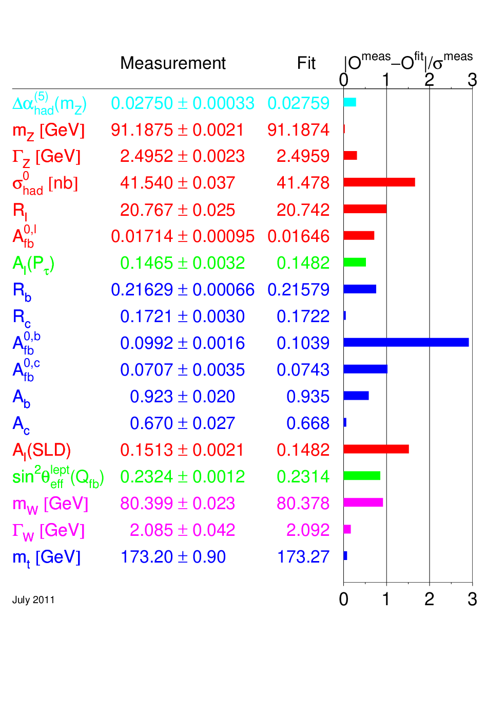
The SM is in good agreement with a very large volume of data. Precision measurements have found no significant deviations from its predictions, with preference for a light Higgs. For instance, EW precision tests performed during the first run of LEP and at SLC have provided accurate measurements of the properties of the neutral current sector. On the other hand, during the second run of LEP, LEP2, the $W$ mass, its decay width and branching ratios were measured with an accuracy of a few parts per ten thousand. Since two of the three tree-level diagrams contributing to $W$ pair production contain triple gauge boson couplings, the non-abelian nature of the EW interactions was also tested there. Further measurements of the $W$ parameters were performed at the Tevatron where, in addition, the $W$ boson can be single produced with a large cross section. Up to now, with the only exception of neutrino oscillations (which require neutrino masses and an extension of the SM), the dark matter problem, and despite a few discrepancies of limited statistical significance, all experimental data are consistent within the SM. Fig. 1.4 illustrates the agreement/disagreement between the experimental measurements and the theoretical predictions for the most significant EW precision observables [32]. It is given in terms of the pulls: the absolute value of the difference between measurement and prediction normalized to the experimental error. The theoretical predictions of the SM for the best fit of $m_{h}$ (Fig. 1.5) have been obtained including all known radiative corrections and using the measured central values of the top quark mass ( $m_{t}$ ), the strong coupling constant ( $\alpha_{s}$ ), etc. The agreement should be considered excellent even if a few measurements show discrepancies between 1 and 3 standard deviations ( $\sigma$ ), which are expected when a large number of observables are included in a fit. On the other hand, these few discrepancies have motivated many analyses that have tried to favor or disregard them as hints for new physics. The most significant of them is probably the anomalous magnetic moment of the muon (not included in the table as it involves hadronic physics and is not usually considered an EW precision observable). It has been computed within the SM at four loops. Combining the data available it is found 1 to 3.2 $\sigma$ away from the SM prediction, depending on whether we use $\tau$ decay data or electron-positron data, respectively. This deviation could be accounted by contributions from new physics such as SUSY with large $\tan\beta$ [33, 34]. Another significant deviation is the bottom forward-backward asymmetry $A^{b}_{FB}$ measured at LEP. The best-fit value gives a prediction which is 2.8 $\sigma$ above its experimental value. This deviation has sometimes been interpreted as a hint of new physics strongly coupled to the third quark family [35, 36]. Supporting this idea, a $3\sigma$ deviation has also been observed in the forward-backward asymmetry in the $t\bar{t}$ production at the Tevatron. We will dedicate the whole Chapter 4 to this point.

As we mentioned before, the Higgs boson mass is an unknown parameter that enters logarithmically in the calculation of these observables at the loop level. Therefore, precision data will put indirect bounds on the value of this parameter. It should be noticed, however, that constraints on $m_{h}$ from EW precision measurements are controversial, as they arise from a combination of measurements that push the SM in different directions. The most constraining observables, besides the $W$ boson mass, are LEP and SLC measurements of leptonic asymmetries ( $A_{LR}$ ) and $A^{b}_{FB}$ . While the former favors a light Higgs boson (as it is also the case for the value of the $W$ boson mass), the hadronic asymmetries prefer a heavier Higgs. Taking into account all the precision EW data given in Fig. 1.4 in a combined fit (Fig. 1.5) it results into $m_{h}\approx 92$ GeV [32], with an experimental uncertainty of $+34$ and $-26$ GeV at 68% confidence level (CL) derived from $\Delta\chi^{2}$ = 1. At 95% of CL precision EW measurements tell us that the mass of the SM Higgs boson is lower than about 161 GeV (including both the experimental and the theoretical uncertainty). This limit increases to 185 GeV when including the LEP2 direct search limit of 114 GeV (shown in light-grey/yellow shaded in Fig. 1.5).

1.6 Constraints on the Higgs mass from direct searches

Before LEP (started in 1989), Higgs masses below 5 GeV were thought to be unlikely. The main probes for $m_{h}\leq 20$ MeV were nuclear-physics experiments with large theoretical uncertainties. Some of these searches were [37]:

1.

For very low Higgs boson masses, the SINDRUM 590 MeV proton cyclotron spectrometer experiment at the PSI (Villigen) investigated the decay of the pion to electron, electron neutrino and Higgs boson that in turn decays into a pair of electrons. It excluded masses in the interval $10\;{\rm MeV}<m_{h}<110\;{\rm MeV}$ [38].
2.

The CERN-Edinburgh-Mainz-Orsay-Pisa-Siegen collaboration at the SPS (CERN) also searched for the decay of a Higgs boson into a pair of electrons in $K^{0}_{L}\rightarrow\pi^{0}h$ . These searches severely constrained $m_{h}$ below 50 MeV [39].
3.

The CLEO experiment at CESR (Ithaca) searched for decays of the Higgs boson into a pair of muons, pions, and kaons produced through the decay $B\rightarrow K^{0}h$ . It excluded the mass range 0.2–3.6 GeV [40].
4.

Finally, the CUSB collaboration at CESR investigated the radiative decay of various states of the $\Upsilon$ into a Higgs boson [41]. The search for a monochromatic photon sample from the decay $\Upsilon\rightarrow\gamma+X$ excluded the range from 2 $m_{\mu}$ up to 5 GeV [42].

Searches at LEP1

The first run of LEP, also called LEP1, covers from 1989 to 1995 at energies close to the Z resonance ( $\sqrt{s}\thicksim M_{Z}$ ). Because of the large production cross section for a low-mass Higgs boson in Z decays, LEP1 provided a very good environment to further exclude small values of $m_{h}$ . The dominant production mode is the Bjorken process (in Fig. 1.6), where the $Z$ boson decays into a real Higgs boson and an off-shell $Z$ boson that then goes into two light fermions, $Z\rightarrow hZ^{*}\rightarrow hf\bar{f}$ . The Higgs boson can also be produced in the decay $Z\rightarrow h\gamma$ , which occurs through triangular loops built-up by heavy fermions and the $W$ boson (in Fig. 1.7). Relative to $Z\rightarrow hf\bar{f}$ , this loop decay process becomes important for masses $m_{h}\geq 60$ GeV, although in this case only a handful of events are expected.

As shown in Fig. 1.2, the Higgs boson in the LEP1 (and also LEP2) mass range decays predominantly into hadrons (mostly $b\bar{b}$ for $m_{h}\gtrsim 10$ GeV) and with a 8% branching ratio into $\tau$ -lepton pairs. Thus, to avoid the large $e^{+}e^{-}\rightarrow$ hadron background, the Higgs boson has been searched for in the two topologies $Z\rightarrow$ ( $h\rightarrow$ hadrons)( $Z^{*}\rightarrow\nu\bar{\nu}$ ), leading to a final state consisting of two acoplanar jets and missing energy, and $Z\rightarrow$ ( $h\rightarrow$ hadrons)( $Z^{*}\rightarrow e^{+}e^{-},\mu^{+}\mu^{-}$ ), with two energetic leptons isolated from the hadronic system. The absence of any Higgs boson signal by the four collaborations at LEP1 [43, 44, 45, 46] set the 95% CL limit $m_{h}\gtrsim 65.2$ GeV. In these channels the Higgs mass will simply be the invariant mass of the system recoiling against the lepton pair. The bounds are independent of Higgs decay modes provided that its coupling to the $Z$ boson is the one predicted in the SM.

Searches at LEP2

The second run of LEP, with a c.o.m. energy of $\sqrt{s}=209$ GeV, covered from 1995 to 2000, when the experiment was closed. In this energy regime the main production channel is Higss-strahlung, with the $e^{-}e^{+}$ pair going into an off-shell $Z$ boson that then decays into a Higgs particle and a real $Z$ boson, $e^{+}e^{-}\rightarrow Z^{*}\rightarrow hZ$ (in Fig. 1.8).

The searches by the different LEP collaborations have been made in many topologies: $e^{+}e^{-}\rightarrow$ ( $h\rightarrow b\bar{b}$ )( $Z^{*}\rightarrow\nu\bar{\nu}$ ) and $e^{+}e^{-}\rightarrow$ ( $h\rightarrow b\bar{b}$ )( $Z^{*}\rightarrow l^{+}l^{-}$ ), like at LEP1, and also $e^{+}e^{-}\rightarrow$ ( $h\rightarrow\tau^{+}\tau^{-}$ )( $Z^{*}\rightarrow b\bar{b}$ ) and $e^{+}e^{-}\rightarrow$ ( $h\rightarrow b\bar{b}$ )( $Z^{*}\rightarrow\tau^{+}\tau^{-}$ ). Combining the results they obtained an exclusion limit [47]

m_{h}>114.4\textrm{ GeV}

(1.14)

at 95% CL (Fig. 1.9). The upper limit was expected to reach $m_{h}>115.3\textrm{ GeV}$ , with the discrepancy coming from a 1.7 $\sigma$ excess (reported initially as a 2.9 $\sigma$ excess) of events that could be indicating a Higgs boson in the vecinity of $m_{h}=116\textrm{ GeV}$ [47]. This anomaly was considered not significant enough to keep taking data and the experiment was terminated as scheduled (a discovery requires a 5 $\sigma$ deviation).

The bound $m_{h}>114.4\textrm{ GeV}$ can be evaded if, for example, the Higgs boson has a weaker couplings $g_{hZZ}$ to the $Z$ boson than in the SM. This would suppress the $e^{+}e^{-}\rightarrow hZ$ cross section and then the number of Higgs events (proportional to $g_{hZZ}^{2}$ ). In Fig. 1.10 we show the 95% CL bound on $m_{h}$ as a function of $\xi=(g_{hZZ}/g^{SM}_{hZZ})$ . Thus, Higgs bosons with $m_{h}\lesssim 80$ GeV and couplings to the $Z$ boson an order of magnitude smaller than in the SM have also been discarded [47]. On the other hand, a non-standard Higgs with half the SM coupling would relax the bound to 95 GeV. We will see in Chapter 2 that in Little Higgs models the Higgs doublet mixes with a singlet, reducing the value of its couplings to the EW gauge bosons.

Searches at Tevatron

The Tevatron data taking covers from 1987 to 2011. It was a $p\bar{p}$ collider with a c.o.m. energy $\sqrt{s}$ = 1.96 TeV. Here we will briefly discuss the most recent results on Higgs searches. In particular, analyses [48] sought Higgs bosons produced with a vector boson ( $q\bar{q}\rightarrow hW/Z$ ), through gluon-gluon fusion ( $gg\rightarrow h$ ), and through vector boson fusion ( $q\bar{q}\rightarrow q^{\prime}\bar{q}^{\prime}h$ ) with an integrated luminosity up to 8.2 fb^-1 at CDF and 8.6 fb^-1 at D $\emptyset$ . The decay modes under study were $h\rightarrow b\bar{b}$ , $h\rightarrow W^{+}W^{-}$ , $h\rightarrow ZZ$ , $h\rightarrow\tau^{+}\tau^{-}$ and $h\rightarrow\gamma\gamma$ . The results of these analyses are summarized in Fig. 1.11.

At 95% CL the upper limits on Higgs boson production are a factor of 1.17, 1.71, and 0.48 times the values of the SM cross section for $m_{h}$ =115 GeV, 140 GeV, and 165 GeV, respectively. The corresponding median upper limits expected in the absence of Higgs boson production are 1.16, 1.16, and 0.57. There is a small ( $\thickapprox$ 1 $\sigma$ ) excess of data events with respect to the background estimation in searches for the Higgs boson in the mass range 125 GeV $<$ $m_{h}$ $<$ 155 GeV. At the 95% CL the region 156 GeV $<$ $m_{h}$ $<$ 177 GeV is excluded.

Searches at LHC

The LHC data taking started in 2010. It is a $pp$ collider with a c.o.m. energy $\sqrt{s}$ = 7 TeV. Here we will discuss the most recent results with the data collected by ATLAS and CMS during 2010 and 2011.

In December of 2011 the CMS collaboration presented their latest results on SM Higgs boson searches [49]. The data amounted to 4.7 fb^-1, meaning that CMS can explore almost the entire mass range above the 114 GeV limit from LEP up to 600 GeV. They combined searches in a number of Higgs decay channels: $h\rightarrow b\bar{b}$ , $h\rightarrow W^{+}W^{-}$ , $h\rightarrow ZZ$ , $h\rightarrow\tau^{+}\tau^{-}$ and $h\rightarrow\gamma\gamma$ (the same as in Tevatron). The preliminary results exclude the existence of a SM Higgs boson in a wide range of masses: 127–600 GeV at 95% CL and 128–525 GeV at 99% CL (Fig. 1.12). A 95% CL exclusion means that the SM Higgs boson with that mass would yield more evidence than that observed in the data at least 95% of the time in a set of repeated experiments.

A SM Higgs boson mass between 115 GeV and 127 GeV is not excluded (Fig. 1.13). Actually, compared to the SM prediction there is an excess of 2 $\sigma$ in this mass region that appears, quite consistently, in five independent channels. With the amount of data collected so far, it is difficult to distinguish between the two hypotheses of existence versus non-existence of a Higgs signal in this low mass region. The observed excess of events could be a statistical fluctuation of the known background processes, either with or without the existence of the SM Higgs boson in this mass range. The larger data samples to be collected in 2012 will reduce the statistical uncertainties and reveal the existence (or not) of the SM Higgs boson in this mass region.

The results presented the same day by the ATLAS collaboration [50] seem to reach an analogous conclusion. They restrict, with up to 4.9 fb^-1, the search for the Higgs boson to the mass range 115–130 GeV (Fig. 1.14). Like CMS, they find an excess in several independent channels compared to the SM prediction, but this is still not conclusive. As the ATLAS spokesperson Fabiola Gianotti said: ‘This excess may be due to a fluctuation, but it could also be something more interesting. We cannot conclude anything at this stage. We need more study and more data. Given the outstanding performance of the LHC this year, we will not need to wait long for enough data and can look forward to resolving this puzzle in 2012’.

Chapter 2 Little Higgs with a light $T$ quark

The hierarchy problem has been the main reason to expect new physics below $\Lambda\approx 1$ TeV. This new physics would extend the range of validity of the model up to larger scales. In particular, extensions like supersymmetry, technicolor or, more recently, extra dimensions could do the job and rise the cut-off of the SM up to the the Planck or the Grand Unification scale.

This point of view, however, has become increasingly uneasy when facing the experimental evidence. Flavor physics, electric dipole moments and other precision EW observables suggest that, if present, the sfermion masses, the technicolor gauge bosons, or the Kaluza-Klein excitations of the standard gauge fields are above 5 TeV [51]. To be effective below the TeV and consistent with the data these models require a per cent fine tuning, whereas the presence of these new particles above 5 TeV implies that nature deals with the Higgs mass parameter first using a mechanism to cancel 30 digits and then playing hide and seek with the last two digits. It may be more consistent either to presume that there should be another reason explaining this little hierarchy between the EW and the scale of new physics or that there is no dynamical mechanism that explains any fine tuning in the Higgs mass parameter [30, 31]. This second possibility has been seriously considered after recent astrophysical and cosmological data have confirmed a non-zero vacuum energy density (the preferred value does not seem to be explained by any dynamics at that scale), and it will be clearly favored if no physics beyond the SM is observed at the LHC.

Little Higgs (LH) models would release this tension by providing an explanation for the gap between the EW scale and the scale of new physics. It is not that LH does not imply physics beyond the SM (it does), but being its objective and its structure more simple it tends to be more consistent with the data than these other fundamental mechanisms. The LH idea of the Higgs as a pseudo-Goldstone boson of an approximate global symmetry broken spontaneously at the TeV scale could be incorporated into a SUSY [52, 53, 54, 55] or a strongly interacting theory [56, 57, 58, 59] to explain the little hierarchy between the Higgs VEV and the SUSY breaking scale or the mass of the composite states. Thus, LH ideas provide an interesting framework with natural cancellations in the scalar sector and new symmetries that protect the EW scale and define consistent models with a cut-off as high as $\Lambda$ $\approx$ 10 TeV, scale where a more fundamental mechanism would manifest. The most important consequence would be that all the new physics to be explored at the LHC would be described by the LH framework.

More precisely, in LH models the scalar sector has a (tree-level) global symmetry that is broken spontaneously at a scale $f\leq 1$ TeV. The SM Higgs doublet is then a Goldstone boson (GB) of the broken symmetry, and remains massless and with a flat potential at that scale. Yukawa and gauge interactions break explicitly the global symmetry. However, the models are built in such a way that the loop diagrams giving non-symmetric contributions must contain at least two different couplings. This collective breaking keeps the Higgs sector free of one-loop quadratic top-quark and gauge contributions (see [60, 61] for a recent review). Two types of models have been extensively considered in the literature: the littlest based on $SU(5)$ [62, 63, 64] and the simplest based on $SU(3)\times SU(3)$ [65, 66]. We will work on the latter in this chapter.

These LH models, however, suffer tensions that push the value of $f$ in different directions. A scale low enough to solve the little hierarchy problem suggests $f\leq 1$ TeV. On the other hand, LH models introduce new gauge vector bosons of mass proportional to $f$ that mix with the EW bosons. This mixing implies $f\geq 3$ TeV in order to be consistent with precision data. The generic solution to this problem proposed in the literature is the presence of a discrete symmetry known as $T$ parity. Such symmetry forbids the mixing of particles of different parity and implies acceptable corrections to the EW observables even for $f\approx 700$ GeV.

In this chapter we will propose an alternative solution. We will see that in the simplest model it is possible to separate the mass of the extra $T$ quark, which is responsible for the cancellation of the dominant top-quark corrections to $\mu^{2}$ , from the mass of the extra vector bosons. A scenario with a 600 GeV $T$ quark and 2 TeV extra gauge bosons would be efficient both to cancel dangerous quadratic corrections and to avoid excessive mixing with the standard vector bosons.

After a short review of the simplest LH model, we show how to accommodate such scenario, and we analyze its phenomenological implications in Higgs and top-quark physics. In addition, we show that the collective breaking of the global symmetry in the original model is not adequate to give an acceptable mass for the Higgs boson. We study the one-loop effective potential and show that an approximate symmetry (as opposed to the one broken collectively) implies the separation between the $T$ and the $Z^{\prime}$ and $W^{\prime}$ masses and could also solve the insufficient value of the Higgs mass in the usual model. This chapter is based on the two publications [2, 3].

2.1 Global symmetries and Goldstone bosons

The generic idea is that the Higgs appears as a GB of a global symmetry broken spontaneously above the EW scale. If the symmetry is exact, the GBs are massless and their couplings are only derivatives. Let us see a few examples as an introduction.

The U(1) case

Consider a theory with a single complex scalar field $\phi$ with potential $V(\phi^{*}\phi)$ invariant under the global $U(1)$ symmetry transformations $\phi\rightarrow e^{i\alpha}\phi\,.$ If the minimum of the potential is at some distance $f$ from the origin we may express $\phi$ as

\phi(x)=\left(f+{r(x)\over\sqrt{2}}\right)e^{i\theta(x)/f}\,.

(2.1)

Rewriting the Lagrangian in terms of these new fields we find that the radial mode $r$ (with mass of order $f$ ) is invariant under $U(1)$ whereas $\theta$ shifts

\theta\rightarrow\theta+\alpha\,.

(2.2)

The potential does not change with $\theta$ (it has a flat direction), implying that $\theta$ is massless and without self-interactions: it is the GB of the broken global symmetry.

The SU(N) case

Generalizing to the non-Abelian case, we will find one GB for each independent broken symmetry. The VEV of a single fundamental field $\phi$ of $SU(N)$ will always break $SU(N)$ to $SU(N-1)$ . Since all the possibilities are equivalent (related by the $SU(N)$ symmetry), we may take the lowest component as the only one with a nontrivial VEV. The number of broken generators is the dimension of $SU(N)$ minus the dimension of $SU(N-1)$ ,

[N^{2}-1]-[(N-1)^{2}-1]=2N-1\,.

(2.3)

The GBs can be parametrized

\phi=e^{i{\pi^{a}(x)T^{a}}/f}\phi_{0}=\exp\left\{{i\over f}\left(\begin{array}[]{c|c}&\pi_{1}\\ &\vdots\\ &\pi_{N-1}\\ \hline\cr\pi^{*}_{1}\cdots\pi_{N-1}^{*}&\pi_{0}/\sqrt{2}\end{array}\right)\right\}\left(\begin{array}[]{c}0\\ \vdots\\ 0\\ f+{r(x)\over\sqrt{2}}\end{array}\right)\equiv e^{i\Pi/f}\phi_{0}\;,

(2.4)

where $\pi^{a}(x)$ are real fields and $T^{a}$ are the generators of the broken symmetries. The field $\pi_{0}$ is real while the fields $\pi_{1}\cdots\pi_{N-1}$ are complex. The last equality defines a convenient short-hand notation. Under an unbroken $SU(N-1)$ transformation the GBs go to

\phi\rightarrow U_{N-1}\ \phi=(U_{N-1}\ e^{i\Pi}\ U_{N-1}^{\dagger})\,U_{N-1}\ \phi_{0}=e^{i(U_{N-1}\,\Pi\,U_{N-1}^{\dagger})}\,\phi_{0}\;,

(2.5)

where we have used that $\phi_{0}$ is invariant under the unbroken $U_{N-1}$ . Therefore, the GBs transform in the usual linear way,

\Pi\rightarrow U_{N-1}\,\Pi\,U_{N-1}^{\dagger}\;.

(2.6)

More explicitly, the unbroken $SU(N-1)$ transformations are

U_{N-1}=\left(\begin{array}[]{cc}\hat{U}_{N-1}&0\\ 0&1\end{array}\right)\;.

(2.7)

The real GB $\pi_{0}$ is then a singlet, whereas the $N\!-\!1$ complex GBs transform as

\displaystyle\left(\begin{array}[]{cc|c}0&&\vec{\pi}\\ &&\\ \hline\cr\vec{\pi}^{\dagger}&&0\end{array}\right)\rightarrow U_{N\!-\!1}\left(\begin{array}[]{cc|c}0&&\vec{\pi}\\ &&\\ \hline\cr\vec{\pi}^{\dagger}&&0\end{array}\right)U_{N\!-\!1}^{\dagger}=\left(\begin{array}[]{cc|c}0&&\hat{U}_{N\!-\!1}\vec{\pi}\\ &&\\ \hline\cr\vec{\pi}^{\dagger}\hat{U}_{N\!-\!1}^{\dagger}&&0\end{array}\right)\;,

where we have used a vector notation $\vec{\pi}$ to represent the $N\!-\!1$ complex GBs as a column vector. Therefore, $\vec{\pi}$ transforms in the fundamental representation of $SU(N-1)$ ,

\vec{\pi}\rightarrow\hat{U}_{N-1}\vec{\pi}\;.

(2.18)

Under the broken symmetry we have

$\displaystyle\phi\rightarrow U\,e^{i\Pi}\,\phi_{0}$	$\displaystyle=$	$\displaystyle\exp\left\{i\left(\begin{array}[]{cc}0&\vec{\alpha}\\ \vec{\alpha}^{\dagger}&0\end{array}\right)\right\}\exp\left\{i\left(\begin{array}[]{cc}0&\vec{\pi}\\ \vec{\pi}^{\dagger}&0\end{array}\right)\right\}\phi_{0}$
	$\displaystyle\equiv$	$\displaystyle\exp\left\{i\left(\begin{array}[]{cc}0&{\vec{\pi}^{\prime}}\\ {{\vec{\pi}^{\prime}}}\,\!^{\dagger}&0\end{array}\right)\right\}U_{N-1}(\vec{\alpha},\vec{\pi})\ \phi_{0}$
	$\displaystyle=$	$\displaystyle\exp\left\{i\left(\begin{array}[]{cc}0&{\vec{\pi}^{\prime}}\\ {{\vec{\pi}}^{\prime}}\,\!^{\dagger}&0\end{array}\right)\right\}\phi_{0}\,,$

where we have used that any $SU(N)$ transformation can be written as the product of a transformation in the coset $SU(N)/SU(N-1)$ times an $SU(N-1)$ transformation. The $U_{N-1}(\vec{\alpha},\vec{\pi})$ transformation, which depends on $\vec{\alpha}$ and $\vec{\pi}$ , leaves $\phi_{0}$ invariant and can therefore be removed. For infinitesimal transformations one obtains

\displaystyle\vec{\pi}\rightarrow\vec{\pi}^{\prime}=\vec{\pi}+\delta\vec{\alpha}\,.

(2.30)

Like in the $U(1)$ case, the shift symmetry ensures that GBs define flat directions in the potential and can only have derivative interactions.

2.2 The simplest Little Higgs model

The scalar sector of the simplest LH model [65] contains two triplets, $\phi_{1}$ and $\phi_{2}$ , under a global $SU(3)_{1}\times SU(3)_{2}\times U(1)_{\chi}$ ¹¹ 1 See the next section to understand the reason to add the $U(1)_{\chi}$ symmetry. symmetry:

\phi_{1}\rightarrow e^{i\theta^{a}_{1}T^{a}}\phi_{1}\;,\;\;\;\;\phi_{2}\rightarrow e^{i\theta^{a}_{2}T^{a}}\phi_{2}\;,

(2.31)

where $T^{a}$ are the $SU(3)$ generators. It is then assumed that these triplets get VEVs $f_{1,2}$ and break the global symmetry to $SU(2)_{1}\times SU(2)_{2}\times U(1)_{Y}$ . The spectrum of scalar fields at this scale will consist of 10 massless modes (the GBs of the broken symmetry) plus two massive fields (with masses of order $f_{1}$ and $f_{2}$ ). In particular, if the two VEVs are

\langle\phi_{1}\rangle=\left(\begin{array}[]{c}0\\ 0\\ f_{1}\end{array}\right)\;,\;\;\;\;\langle\phi_{2}\rangle=\left(\begin{array}[]{c}0\\ 0\\ f_{2}\end{array}\right)\;,

(2.32)

it is possible to parametrize the fields like

\phi_{1}=e^{+i\Theta^{\prime}}e^{+i\;{f_{2}\over f_{1}}\Theta}\left(\begin{array}[]{c}0\\ 0\\ f_{1}+\displaystyle{r_{1}\over\sqrt{2}}\end{array}\right)\,,\;\;\;\phi_{2}=e^{+i\Theta^{\prime}}e^{-i\;{f_{1}\over f_{2}}\Theta}\left(\begin{array}[]{c}0\\ 0\\ f_{2}+\displaystyle{r_{2}\over\sqrt{2}}\end{array}\right)\,,

(2.33)

where

\Theta^{\prime}={1\over f}\,\left(\begin{array}[]{ccc}\eta^{\prime}/\sqrt{3}&0&h^{\prime}\\ 0&\eta^{\prime}/\sqrt{3}&\hat{h}\\ h^{{}^{\prime}\dagger}&\hat{h}^{\dagger}&-2\eta^{\prime}/\sqrt{3}\end{array}\right)\,,\;\;\Theta={1\over f}\;\left(\begin{array}[]{ccc}\eta/\sqrt{2}&0&h^{0}\\ 0&\eta/\sqrt{2}&h^{-}\\ h^{0\dagger}&h^{+}&\eta/\sqrt{2}\end{array}\right)\,,

(2.34)

$f=\sqrt{f_{1}^{2}+f_{2}^{2}}$ and $r_{1,2}$ are massive scalars of order $f_{1,2}$ , respectively.

If now, in order to remove some of the GBs, the diagonal combination of $SU(3)_{1}\times SU(3)_{2}$ and the $U(1)_{\chi}$ are made local, i.e.,

\phi_{1(2)}\rightarrow e^{i\theta^{a}(x)T^{a}}\phi_{1(2)}\;,

(2.35)

then the VEVs also break the local symmetry $SU(3)_{L}\times U(1)_{\chi}$ to the SM group $SU(2)_{L}\times U(1)_{Y}$ . In the unitary gauge, 5 GBs, the ones in $\Theta^{\prime}$ , disappear. The other 5 GBs (the complex doublet $(h^{0}\;h^{-})$ and the CP-odd $\eta$ ) are parametrized as

\phi_{1}=e^{+i\;{f_{2}\over f_{1}}\Theta(x)}\left(\begin{array}[]{c}0\\ 0\\ f_{1}+\displaystyle{r_{1}\over\sqrt{2}}\end{array}\right)\;,\;\;\;\;\phi_{2}=e^{-i\;{f_{1}\over f_{2}}\Theta(x)}\left(\begin{array}[]{c}0\\ 0\\ f_{2}+\displaystyle{r_{2}\over\sqrt{2}}\end{array}\right)\,,

(2.36)

with $\Theta(x)$ defined in Eq.(2.34).

Color and hypercharge

The addition of the gauge $SU(3)_{C}$ symmetry is straightforward. The hypercharge results from the combination

Y={-1\over\sqrt{3}}T^{8}+X\,,

(2.37)

where $X$ is the generator of $U(1)_{\chi}$ and $T^{8}$ the charge

\displaystyle T^{8}={1\over 2\sqrt{3}}\left(\begin{array}[]{ccc}1&&\\ &1&\\ &&-2\end{array}\right)\,

in $SU(3)_{L}$ . With this embedding of the SM symmetry the components in a $SU(3)$ triplet are

\phi_{i}={\bf 3}_{-1/3}=\left(\begin{array}[]{c}\phi^{0}\\ \phi^{-}\\ s^{0}\end{array}\right)\,.

(2.42)

Exotic matter content

The fermion content must be accommodated in complete multiples of the local $SU(3)_{C}\times SU(3)_{L}\times U(1)_{\chi}$ gauge symmetry. In particular, the $SU(2)_{L}$ doublets become triplets:

\left(\begin{array}[]{c}t\\ b\end{array}\right),\;\left(\begin{array}[]{c}\nu\\ e\end{array}\right)\;\;\longrightarrow\;\;\Psi_{Q}=\left(\begin{array}[]{c}t\\ b\\ T\end{array}\right),\;\Psi_{L}=\left(\begin{array}[]{c}\nu\\ e\\ N\end{array}\right)\;,

(2.43)

where $T$ and $N$ are singlets under $SU(2)_{L}$ with electric charge $Q_{T}=\frac{2}{3}$ and $Q_{N}=0$ , respectively. The Yukawa sector must give these extra fields a mass at the scale $f$ . To see how it works, we will just discuss the third family, being the arguments for the lighter generations analogous. Instead of a quark singlet $t^{c}$ we will add two of them, $t^{c}_{1}$ and $t^{c}_{2}$ , together with a neutral lepton singlet $n^{c}$ .

$(i)$ In the top-quark sector one assumes

-{\cal L}_{t}=\lambda_{1}\;\phi_{1}^{\dagger}\Psi_{Q}t_{1}^{c}+\lambda_{2}\;\phi_{2}^{\dagger}\Psi_{Q}t_{2}^{c}+{\rm h.c.}\;,

(2.44)

where, from now on, all fermions are two-component spinors. As we will see in the next section, these two Yukawas are necessary to give mass both to the top and the $T$ quarks. Moreover, if $\lambda_{1}$ or $\lambda_{2}$ were zero the global symmetry protecting the Higgs mass would be exact in this sector. Therefore, diagrams containing only one of the two couplings do not break the symmetry and do not contribute to $\mu^{2}$ .

This mechanism is known as collective symmetry breaking. The one-loop diagram in Fig. 2.2 breaks the global $SU(3)_{1}\times SU(3)_{2}$ symmetry and would introduce quadratic contributions to $\mu^{2}$ , but it is absent if $\lambda_{1,2}$ are the only non-zero couplings. At one loop the dominant contribution to $\mu^{2}$ comes from the diagram in Fig. 2.3, which introduces a logarithmic correction $\sim m_{T}^{2}\ln\Lambda$ that would be acceptable.

$(ii)$ The lepton sector with a massive $N$ reads,

-{\cal L}_{\nu}=\lambda^{\nu}_{1}\;\phi_{1}^{\dagger}\Psi_{L}n^{c}+{\rm h.c.}\;.

(2.45)

Diagrams with either $\phi_{1}$ or $\phi_{2}$ are allowed, but not both simultaneously. If both terms appear we would find diagrams of the kind of Fig. 2.4 giving quadratic contributions to $\mu^{2}$ .

Summarizing, the matter content is three families with quantum numbers under $SU(3)_{C}\times SU(3)_{L}\times U(1)_{\chi}$ :

\displaystyle\begin{array}[]{cc}\Psi_{Q}=({\bf 3},{\bf 3})_{1\over 3}&\Psi_{L}=({\bf 1},{\bf 3})_{-{1\over 3}}\\ b^{c}=({\bf\bar{3}},{\bf 1})_{1\over 3}&e^{c}=({\bf 1},{\bf 1})_{1}\\ 2\times t^{c}=({\bf\bar{3}},{\bf 1})_{-{2\over 3}}&n^{c}=({\bf 1},{\bf 1})_{0}\end{array}

In the gauge-boson sector we have 8 massive particles plus the photon as the $SU(3)_{L}\times U(1)_{X}$ symmetry breaks into $U(1)_{EM}$ . Five of these massive vector fields are neutral and the other four are charged. Of course, the EW gauge bosons are included among them.

2.3 A light $T$ quark

The purpose of Little Higgs models is to protect the mass squared of the Higgs from one-loop quadratic contributions using a global symmetry, rising the natural cut-off of the theory up to $\approx 10$ TeV. This requires an extra $T$ quark lighter than 1 TeV. On the other hand, the extra vector bosons that have been introduced to absorb the extra GBs of the global symmetry must be heavy enough to avoid unacceptable four fermion operators and, specially, a too large mixing with the EW gauge bosons. The value of this mixing is very constrained by LEP data and other precision experiments and requires $f=\sqrt{f_{1}^{2}+f_{2}^{2}}\geq 3$ TeV [65, 67, 68, 69]. However, this condition is not necessarily fulfilled with two VEVs of the same order; one could have, for example, $f_{2}\geq 3$ TeV and the other VEV significantly smaller. It turns out that in order to keep a light $T$ quark the latter choice is more convenient. At the scale $f$ and neglecting the EW VEV Eq.(2.44) implies a massless top quark and a $T$ quark with mass $m_{T}$ :

-{\cal L}_{t}\supset\lambda_{1}\;f_{1}Tt_{1}^{c}+\lambda_{2}\;f_{2}Tt_{2}^{c}+{\rm h.c.}=m_{T}\;TT^{c}+{\rm h.c.}\;,

(2.50)

where $m_{T}=\sqrt{\lambda_{1}^{2}f_{1}^{2}+\lambda_{2}^{2}f_{2}^{2}}$ and $\;T^{c}=s_{\alpha}\;t_{1}^{c}+c_{\alpha}\;t_{2}^{c}$ , with $s_{\alpha}=\lambda_{1}f_{1}/\sqrt{\lambda_{1}^{2}f_{1}^{2}+\lambda_{2}^{2}f_{2}^{2}}$ . To obtain a mass for the $T$ quark smaller than $f$ is possible if $f_{1}\ll f_{2}$ and $\lambda_{2}\ll\lambda_{1}$ . Once the Higgs field gets a VEV, the top quark mixes with the extra $T$ quark defining the mass eigenstates

t^{\prime}=c_{\theta}\;t-s_{\theta}\;T\;,\;\;\;\;T^{\prime}=s_{\theta}\;t+c_{\theta}\;T\;,

(2.51)

where we denote $V_{Tb}\equiv s_{\theta}$ .

The mixing of $T$ with the top quark introduces gauge couplings with the $W$ and $Z$ bosons for the extra $T$ quark:

	$\displaystyle{\cal L}_{W}$	$\displaystyle=$	$\displaystyle-{g\over\sqrt{2}}\;\overline{t}\sigma^{\mu}b\;W^{+}_{\mu}+{\rm h.c.}$		(2.52)
		$\displaystyle=$	$\displaystyle-{g\over\sqrt{2}}\left(\sqrt{1-V^{2}_{Tb}}\;\overline{t}^{\prime}\sigma^{\mu}b+V_{Tb}\;\overline{T}^{\prime}\sigma^{\mu}b\right)W^{+}_{\mu}+{\rm h.c.}\;,$		(2.52)

	$\displaystyle{\cal L}_{Z}$	$\displaystyle\supset$	$\displaystyle-{g\over 2c_{W}}\left({\begin{array}[]{cc}\overline{t}&\overline{T}\\ \end{array}}\right)\sigma^{\mu}\left({\begin{array}[]{cc}1&0\\ 0&0\\ \end{array}}\right)\left({\begin{array}[]{c}t\\ T\\ \end{array}}\right)Z_{\mu}$
		$\displaystyle\approx$	$\displaystyle-{g\over 2c_{W}}\left({\begin{array}[]{cc}\overline{t}^{\prime}&\overline{T}^{\prime}\\ \end{array}}\right)\sigma^{\mu}\left({\begin{array}[]{cc}1-V^{2}_{Tb}&V_{Tb}\\ V_{Tb}&V^{2}_{Tb}\\ \end{array}}\right)\left({\begin{array}[]{c}t^{\prime}\\ T^{\prime}\\ \end{array}}\right)Z_{\mu}\;.$

As we see, we obtain top-quark flavor-changing neutral currents coupled to the $Z$ boson. This same kind of currents also appear in Yukawa couplings with the Higgs boson. In this regard, it is important to mention that in models with a vectorlike $T$ quark it is usually assumed that $T$ couples to the Higgs boson only through mixing with the top quark. This implies a Yukawa coupling $V_{Tb}m_{T}/v$ [70]. In our model, however, the Higgs couples to $T$ and $T^{c}$ even if the mixing term $V_{Tb}$ is zero, since $h$ includes an order $m_{t}/m_{T}$ singlet component (see next section).

The presence of a $T$ quark has phenomenological consequences. In [70] Aguilar-Saavedra discusses the constraints on $V_{Tb}$ from precision observables as a function of the $T$ -quark mass (see Fig. 2.5). It is remarkable that the limits vanish when $m_{T}\rightarrow m_{t}$ ; a heavier $T$ quark would take (through mixing) part of the $t$ quark interaction to the EW bosons changing the standard corrections to EW observables.

2.4 Little Higgs or extra singlet model?

To break the EW symmetry the Higgs field $h^{0}$ has to get a potential (see next sections) defining a non-zero VEV

\langle h^{0}\rangle=u/\sqrt{2}\;.

(2.65)

This would translate into the following triplet VEVs:

\langle\phi_{1}\rangle=e^{+i\;{f_{2}\over f_{1}}\langle\Theta\rangle}\left(\begin{array}[]{c}0\\ 0\\ f_{1}\end{array}\right)\;,\;\;\;\;\langle\phi_{2}\rangle=e^{-i\;{f_{1}\over f_{2}}\langle\Theta\rangle}\left(\begin{array}[]{c}0\\ 0\\ f_{2}\end{array}\right)\;,

(2.66)

where

\langle\Theta\rangle={1\over f}\;\left(\begin{array}[]{ccc}0&0&u/\sqrt{2}\\ 0&0&0\\ u/\sqrt{2}&0&0\end{array}\right)\ \;.

(2.67)

Working out the expression we obtain

\langle\phi_{1}\rangle=\left(\begin{array}[]{c}if_{1}s_{1}\\ 0\\ f_{1}c_{1}\end{array}\right)\;,\;\;\;\;\langle\phi_{2}\rangle=\left(\begin{array}[]{c}-if_{2}s_{2}\\ 0\\ f_{2}c_{2}\end{array}\right)\;,

(2.68)

with

s_{1}\equiv\sin{uf_{2}\over\sqrt{2}ff_{1}}\;,\;\;\;\;s_{2}\equiv\sin{uf_{1}\over\sqrt{2}ff_{2}}\;.

(2.69)

In previous literature the way to carry out this point has usually been through a first order approximation

\langle\phi_{1}\rangle\sim\left(\begin{array}[]{c}iuf_{2}\over{\sqrt{2}f}\\ 0\\ f_{1}\end{array}\right)\;,\;\;\;\;\langle\phi_{2}\rangle\sim\left(\begin{array}[]{c}-iuf_{1}\over{\sqrt{2}f}\\ 0\\ f_{2}\end{array}\right)\;,

(2.70)

that may not be good if $f\approx f_{2}\gg f_{1}>u/\sqrt{2}$ and that would make our argument below less apparent.

Since the upper components of the triplets transform as a $SU(2)_{L}$ doublet, it is clear that in order to get the mass of the $W$ and $Z$ bosons we need

\sqrt{f_{1}^{2}s_{1}^{2}+f_{2}^{2}s_{2}^{2}}={v\over\sqrt{2}}\approx 174\;{\rm GeV}\;.

(2.71)

If $f\approx f_{2}\gg f_{1}$ we obtain

s_{1}\approx\sin{u\over\sqrt{2}f_{1}}\;,\;\;\;\;s_{2}\approx{uf_{1}\over\sqrt{2}f^{2}}\;,

(2.72)

and the EW scale would just be

{v\over\sqrt{2}}\approx f_{1}s_{1}\;.

(2.73)

The Higgs $h$ is obtained expanding $h^{0}$ (in the unitary gauge) as $h^{0}=(u+h)/\sqrt{2}$ . We find that $h$ has a singlet and a doublet component:

\phi_{1}=\left(\begin{array}[]{c}if_{1}(s_{1}\cos\displaystyle{h\over\sqrt{2}f_{1}}+c_{1}\sin\displaystyle{h\over\sqrt{2}f_{1}})\\ 0\\ f_{1}(c_{1}\cos\displaystyle{h\over\sqrt{2}f_{1}}-s_{1}\sin\displaystyle{h\over\sqrt{2}f_{1}})\end{array}\right)\approx\displaystyle{1\over\sqrt{2}}\left(\begin{array}[]{c}ic_{1}h\\ 0\\ -s_{1}h\end{array}\right)+...

(2.74)

If $f_{1}$ is much larger than the EW scale, $s_{1}$ will be small and $h$ mainly a doublet. However, if $f_{1}$ is $\sim v/\sqrt{2}$ , the singlet component $s_{1}$ grows large. In this case, the doublet component lost by $h$ becomes part of the radial scalar $r_{1}$ whose mass is $\sim f_{1}$ .

This is a generic issue of the LH models. The scale $f$ of a broken global symmetry is always defined by the VEV of a $SU(2)_{L}$ singlet, implying a massive mode (a radial singlet of mass $m_{r}\sim f$ ) in addition to the GBs (the Higgs). Then, the EW symmetry breaking mixes the Higgs with this massive singlet. This mechanism is at work in any framework were the Higgs is a pseudo-GB of a global symmetry, including composite Higgs models: the resulting Higgs will always include a singlet component of order $v/(\sqrt{2}f)$ . In our model the effect is even more relevant because the scale of global symmetry breaking is split in two, $f_{1}$ and $f_{2}$ , and it is the lighter VEV the one defining the singlet component.

Let us now see the consequences of having a singlet component in the Higgs field. We consider a Higgs field $h$ and a massive scalar $r_{1}$ that include both $SU(2)_{L}$ doublet $d$ and singlet $s$ components:

	$\displaystyle d$	$\displaystyle=$	$\displaystyle c_{1}h+s_{1}r_{1}$
	$\displaystyle s$	$\displaystyle=$	$\displaystyle-s_{1}h+c_{1}r_{1}$		(2.75)

The scalar $h$ gets a VEV $u$ , but the $Z$ boson only couples to the doublet component in $h$ (suppressed by a factor of $c_{1}^{2}$ ), getting a mass

{\cal L}\supset\frac{g^{2}\langle h\rangle^{2}c_{1}^{2}}{8\cos^{2}\theta_{W}}Z_{\mu}Z^{\mu}

(2.76)

To fit the measured value of $M_{Z}$ the Higgs VEV $u$ must be larger than the one ( $v$ ) in the SM, to compensate the appearance of the cosine multiplying:

\langle h\rangle=u=\frac{v}{c_{1}}

(2.77)

The gauge coupling of the $Z$ boson with the Higgs boson appears suppressed (see Fig. 2.6):

{\cal L}\supset\frac{g^{2}h^{2}c_{1}^{2}}{8cos^{2}\theta_{W}}Z_{\mu}Z^{\mu}\;,

(2.78)

i.e.,

\frac{g}{g^{SM}}=c_{1}\;.

(2.79)

The same consequence is deduced from the mass of the $W$ boson (the $\rho=M_{W}^{2}/M_{Z}^{2}\cos^{2}\theta_{W}$ parameter does not change) and the coupling to the Higgs boson.

In the Yukawa top-quark sector we have

	$\displaystyle{-\cal L}$	$\displaystyle\supset$	$\displaystyle\frac{y_{t}}{\sqrt{2}}dtt^{c}+h.c.$		(2.80)
		$\displaystyle=$	$\displaystyle\frac{y_{t}}{\sqrt{2}}\left(c_{1}\left(u+h\right)+s_{1}r_{1}\right)+h.c.\;,$		(2.80)

which implies

m_{t}=\frac{y_{t}c_{1}u}{\sqrt{2}}

(2.81)

and

{-\cal L}\supset m_{t}tt^{c}+\frac{m_{t}}{v}c_{1}htt^{c}\,.

(2.82)

Therefore, the top-quark Yukawa coupling is also suppressed by a factor $c_{1}$ respect to the value in the SM.

Summarizing, since the singlet component of $h$ does not couple, both its gauge ( $g$ and $g^{\prime}$ ) and Yukawa ( $\sqrt{2}m_{f}/v$ ) couplings will appear suppressed by a factor of $c_{1}$ . These anomalous LH couplings have nothing to do with the non-linear realization of the scalar fields, they just reflect the mixing with the scalar singlet massive at the scale of the global symmetry breaking. As we mentioned above, in our case $f_{1}$ can be close to $v/\sqrt{2}$ while consistent with all precision data, and the effect may be large enough to be observable at the LHC.

Notice also that the Little Higgs $h$ , not being a pure doublet, only unitarizes partially the SM cross sections involving massive vector bosons. In particular, the cut-off at $\approx 1$ TeV set by $WW$ elastic scattering would be moved up to (1/ $s_{1}$ ) TeV. Below that scale the massive scalar $r_{1}$ (or a techni- $\rho$ in composite models) should complete the unitarization.

A final comment concerns the limit $f_{1}\rightarrow v/\sqrt{2}$ . The GB $h$ becomes there a pure $SU(2)_{L}$ singlet, and the (unprotected) field $r_{1}$ , massive at the scale $f_{1}$ , becomes a doublet and is the real Higgs that breaks the EW symmetry. In this limit, the natural cut-off would be the same as in the SM, whereas in the general case with $f_{1}>v/\sqrt{2}$ it is at $\approx 4\pi f_{1}$ .

2.5 Phenomenology

The three basic ingredients of the LH models under study here are the presence of heavy vector bosons, a relatively light $T$ quark, and a sizable singlet component in the Higgs field. A fourth ingredient, the presence of the $CP$ -odd light scalar $\eta$ (in Eq. (2.34)), also a GB of the global symmetry, seems more model dependent (see next section). Let us briefly analyze the phenomenological consequences of these ingredients.

1.

Effects on EW precision observables.

$(i)$ The massive gauge bosons would introduce mixing with the standard bosons and four fermion operators. This could manifest as a shift in the $Z$ mass and other precision data. However, none of these effects is observable if $f_{2}\geq 3$ TeV [65].

$(ii)$ The effects on EW precision observables due to the singlet component of the Higgs field are also negligible even if the extra scalar $r_{1}$ is heavier than the Higgs boson. Although the Yukawa coupling of the top with the neutral Higgs is here smaller than in the SM, it is the coupling with the would be GBs (the scalars eaten by the $W$ and $Z$ bosons) what determines the large top quark radiative corrections, and these are not affected by the presence of singlets.

$(iii)$ The bounds on a vectorlike $T$ quark from precision EW data have been extensively studied in the literature, we will comment here the results in [70] as they apply to LH models in a straightforward way.

The mixing of the top quark with the $T$ singlet reduces its coupling with the $Z$ boson. This, in turn, affects the top quark radiative corrections (triangle diagrams) to the $Zbb$ vertex, which is measured in the partial width $Z$ to $b\overline{b}$ [ $R_{b}=\Gamma(Z\rightarrow b\overline{b})/\Gamma(Z\rightarrow{\rm hadrons})$ ] and forward-backward asymmetries. The heavier $T$ quark also gives this type of corrections to the $Zbb$ vertex, and for low values of $m_{T}$ both effects tend to cancel (i.e., if $m_{T}=m_{t}$ the vertex $Zbb$ is the same as in the SM). For large values of $m_{T}$ (above 500 GeV) the upper bound on $V_{Tb}$ from precision $b$ physics is around 0.2 [70].

The $T$ quark would also appear in vacuum polarization diagrams, affecting the oblique parameters $S$ , $T$ , and $U$ . For degenerate masses ( $m_{T}=m_{t}$ ) the corrections to $T$ and $U$ vanish for any value of the mixing $V_{Tb}$ and the correction to $S$ is small ( $\Delta S\approx-0.16V_{Tb}$ ). For large values of $m_{T}$ the only oblique parameter with a sizable correction is $T$ ( $\Delta T\approx 2.7V_{Tb}$ for $m_{T}=500$ GeV), but the limits on $V_{Tb}$ are in this case smaller than the ones from $R_{b}$ [70].

The phenomenological impact of these models on Higgs physics at hadron colliders may be important. The main effects can be summarized as follows.

$(i)$ Suppression of the $gg\rightarrow h$ cross section (Fig. 2.7). This effect is due to the suppression of the top-quark Yukawa coupling relative to the SM value (see Fig. 2.6) and also to the contribution of the extra $T$ quark. Although this second factor is numerically less important, it is remarkable that always interferes destructively in the amplitude: the relative minus sign versus the top-quark contribution follows from the cancellation of quadratic corrections to the Higgs mass parameter.

It is easy to obtain approximate expressions for this suppression factor in the limit of $m_{h}\ll m_{t},m_{T}$ [71, 72]:

$\displaystyle R_{gg}\equiv{\sigma(gg\rightarrow h)\over\sigma^{SM}(gg\rightarrow h)}$	$\displaystyle\approx$	$\displaystyle\left({y_{t}\over y_{t}^{SM}}+{y_{T}v\over m_{T}}\right)^{2}$	(2.83)
	$\displaystyle\approx$	$\displaystyle\left(c_{1}c_{\theta}+s_{1}s_{\theta}-t_{1}s^{2}_{\alpha}(s_{1}c_{\theta}-c_{1}s_{\theta})\right)^{2}$
	$\displaystyle\approx$	$\displaystyle c_{1}^{2}$

In Fig. 2.8 we plot the ratio $R_{gg}\equiv\sigma(gg\rightarrow h)/\sigma^{SM}(gg\rightarrow h)$ for different values of $V_{Tb}$ and $m_{T}$ . For $m_{h}=150$ GeV the approximation above is good at the $1\%$ level. This effect, which could hide the Higgs at the LHC, has been recently discussed in general models with scalar singlets [73, 74] and also in the framework of LH models with $T$ parity [75].

$(ii)$ Suppression in the production cross sections that involve gauge interactions: $WW\rightarrow h$ , $q\overline{q}\rightarrow Wh$ , etc. (Fig 2.9). In Fig. 2.8 we also plot the ratio $R_{WW}\equiv\sigma(WW\rightarrow h)/\sigma^{SM}(WW\rightarrow h)\approx c_{1}^{2}$ . It is remarkable that for $m_{h}=150$ GeV the suppression in these cross sections coincides with the one in $\sigma(gg\rightarrow h)$ at the $1\%$ level.

$(iii)$ New production channels through $T$ -quark decay [76]. A $T$ quark of mass below 600 GeV will be copiously produced at the LHC. In particular, the cross section to produce $T\overline{T}$ pairs in $pp$ collisions goes from $10^{4}$ fb for $m_{T}=400$ GeV to $10^{3}$ fb for $m_{T}=600$ GeV [77, 78]. Once produced, a $T$ quark may decay into $Wb$ , $Zt$ , $ht$ and $\eta t$ [79, 80]. We find an approximate relation among the partial widths in the limit of $m_{T}$ much larger than the mass of the final particles:

	$\displaystyle\Gamma(T\rightarrow Wb)\approx{\alpha\over 16s_{W}^{2}}\;V_{Tb}^{2}\;{m_{T}^{3}\over M_{W}^{2}}$
	$\displaystyle\Gamma(T\rightarrow Zt)\approx{1\over 2}\;\Gamma(T\rightarrow Wb)$
	$\displaystyle\Gamma(T\rightarrow ht)\approx{1\over 2}\;(c_{1}^{2}+{s_{1}^{2}\over t_{\alpha}^{2}})\;\Gamma(T\rightarrow Wb)$
	$\displaystyle\Gamma(T\rightarrow\eta t)\approx{1\over 2}\;(s_{1}^{2}+{c_{1}^{2}\over t_{\alpha}^{2}})\;\Gamma(T\rightarrow Wb)$		(2.84)

Notice that the $T$ quark will decay through the 4 channels with branching ratios that are independent of $V_{Tb}$ . $T\rightarrow W^{+}b$ gives the best discovery potential for the $T$ quark, whereas the Higgs $h$ will be produced with a branching ratio close to the $20\%$ . The detailed signal and background study at the LHC in [77, 78] shows that $T\overline{T}\rightarrow W^{+}b\overline{t}h\rightarrow W^{+}bW^{-}\overline{b}h$ and $T\overline{T}\rightarrow hth\overline{t}\rightarrow W^{+}bW^{-}\overline{b}hh$ give a very high statistical significance for the Higgs (around $10\sigma$ for 30 fb^-1). We expect similar results in this model, although the presence of the scalar $\eta$ can open new decay channels for the Higgs. In particular, if $m_{h}>2m_{\eta}$ the coupling $h\eta\eta$ opens the interesting channel $h\rightarrow\eta\eta\rightarrow 4b$ [81] that, together with the suppression in the $hZZ$ coupling, could loosen considerably the 114 GeV LEP bound on the Higgs mass.

2.6 Global symmetry breaking effects and effective potential

In LH models the global symmetry is not exact, it is broken at the one-loop level. These loop corrections generate a potential for the GBs that should imply the right EW VEV and an acceptable mass for the Higgs boson and for the extra $\eta$ scalar. In this section we study the one-loop effective potential for these fields in the usual simplest LH model with collective symmetry breaking. We will show that such model is not able to accommodate the splitting of $f_{1}$ and $f_{2}$ together with an acceptable Higgs potential, and in the next section we will propose a variation of the model.

The one-loop effective potential (or Coleman-Weinberg potential) [82] for $h$ and $\eta$ can be expressed in terms of the masses that the different fields would get if these scalars grow a VEV. Therefore, we will start finding the mass-eigenstates of both the fermion and the gauge boson sectors.

Fermion masses

We will just consider the top-quark sector, as the lighter fermions give negligible contributions. In the case with collective breaking the Yukawas read

-{\cal L}_{t}=\lambda_{1}\;\phi_{1}^{\dagger}\Psi_{Q}t_{1}^{c}+\lambda_{2}\;\phi_{2}^{\dagger}\Psi_{Q}t_{2}^{c}+{\rm h.c.}\;,

(2.85)

Once the Higgs gets a VEV we find the mass matrix

-{\cal L}_{t}\supset\left(\begin{array}[]{cc}t&T\end{array}\right)\left(\begin{array}[]{cc}\lambda_{1}f_{1}s_{1}&-\lambda_{2}f_{2}s_{2}\\ \lambda_{1}f_{1}c_{1}&\lambda_{2}f_{2}c_{2}\end{array}\right)\left(\begin{array}[]{c}t_{1}^{c}\\ t_{2}^{c}\end{array}\right)\,,

(2.86)

with

s_{1}(h)=\sin{hf_{2}\over\sqrt{2}ff_{1}}\;,\;\;\;\;s_{2}(h)=\sin{hf_{1}\over\sqrt{2}ff_{2}}\;.

(2.87)

This expression is independent of the VEV of the $\eta$ field, which appears as a phase that can be absorbed by the fields and thus remains massless.

Working out the diagonalization we find the masses of the top and the $T$ quarks:

m_{t(T)}^{2}(h)={M^{2}\over 2}\left(1-(+)\sqrt{1-s_{2\alpha}^{2}\;s_{12}^{2}(h)}\right)\;,

(2.88)

where

$\displaystyle s_{12}(h)$	$\displaystyle=$	$\displaystyle\sin{hf\over\sqrt{2}f_{1}f_{2}}\;,$
$\displaystyle M^{2}$	$\displaystyle=$	$\displaystyle\lambda_{1}^{2}f_{1}^{2}+\lambda_{2}^{2}f_{2}^{2}\;,$
$\displaystyle s_{2\alpha}$	$\displaystyle=$	$\displaystyle{2\lambda_{1}\lambda_{2}f_{1}f_{2}\over\lambda_{1}^{2}f_{1}^{2}+\lambda_{2}^{2}f_{2}^{2}}\;.$	(2.89)

The Coleman-Weinberg expression for the fermion contribution to the one-loop potential is

V_{top}=-{3\over 16\pi^{2}}\Lambda^{2}\;{\rm Tr}\;[m^{\dagger}m]+{3\over 16\pi^{2}}\;{\rm Tr}\;[(m^{\dagger}m)^{2}\log\left(\Lambda^{2}\over m^{2}\right)]\;.

(2.90)

The global symmetry has some important implications on $V_{top}$ . First of all, ${\rm Tr}\;[m^{\dagger}m]=m_{t}^{2}+m_{T}^{2}$ is a constant (it does not depend on $h$ ), so the quadratic contribution is zero. Moreover, up to a constant we can write

V_{top}={3\over 16\pi^{2}}m_{t}^{4}\log\left(m_{T}^{2}\over m_{t}^{2}\right)+{3\over 16\pi^{2}}\left(m_{t}^{4}+m_{T}^{4}\right)\log\left(\Lambda^{2}\over m_{T}^{2}\right)\,.

(2.91)

This potential can be understood as the usual top quark quartic correction below $m_{T}$ plus a contribution proportional to

m_{t}^{4}+m_{T}^{4}={M^{4}\over 2}\left(2-s^{2}_{2\alpha}\right)\;s_{12}^{2}(h)

(2.92)

above that scale. The latter contribution is logarithmically divergent and it will redefine (renormalize) the quartic coupling to

a\;\left(\phi_{1}^{\dagger}\phi_{2}\right)_{\bf 1}\left(\phi_{2}^{\dagger}\phi_{1}\right)_{\bf 1}\supset a\;f_{1}^{2}f_{2}^{2}\;\left(1-s_{12}^{2}(h)\right)\;.

where the subindex $1$ indicates that the triplets are combined into a $SU(3)$ singlet. The sensibility of the potential to the ultraviolet physics can be taken into account considering $a$ as a free parameter or, equivalently, taking $a=0$ and varying the cut-off freely.

Gauge boson masses

All the masses come from the covariant kinetic terms $(D^{\mu}\Phi_{i})^{\dagger}(D_{\mu}\Phi_{i})$ of the triplets $\Phi_{1,2}$ . We will separate the study of the charged and the neutral gauge bosons.

$(i)$ In the charged sector we have

D_{\mu}\phi_{1}\supset-ig\sum_{i=1,2,6,7}A^{i}_{\mu}T^{i}\phi_{1}={gf_{1}\over\sqrt{2}}\left(\begin{array}[]{c}0\\ s_{1}W_{\mu}-c_{1}W^{\prime}_{\mu}\\ 0\end{array}\right)\;,

(2.93)

where we have defined

W={1\over\sqrt{2}}\left(A^{1}_{\mu}+iA^{2}_{\mu}\right)\;,\;\;W^{\prime}={1\over\sqrt{2}}\left(A^{7}_{\mu}+iA^{6}_{\mu}\right)\;,

(2.94)

with an analogous expression for $D_{\mu}\phi_{2}$ . In this basis the mass matrix reads

{g^{2}\over 2}\left(\begin{array}[]{cc}f_{1}^{2}s_{1}^{2}+f_{2}^{2}s_{2}^{2}&f_{2}^{2}s_{2}c_{2}-f_{1}^{2}s_{1}c_{1}\\ f_{2}^{2}s_{2}c_{2}-f_{1}^{2}s_{1}c_{1}&f_{1}^{2}c_{1}^{2}+f_{2}^{2}c_{2}^{2}\end{array}\right)\;,

(2.95)

and has the eigenvalues

M^{2}_{W_{1}(W_{2})}={g^{2}f^{2}\over 4}\left(1-(+)\sqrt{1-s_{2\beta}^{2}\;s_{12}^{2}}\right)\;,

(2.96)

where

s_{2\beta}\equiv 2{f_{1}f_{2}\over f^{2}}\;.

(2.97)

Notice that, again, the two masses add to a constant independent of the Higgs VEV (in $s_{1,2}$ ), which will imply no quadratic divergences in the potential at the one-loop level.

$(ii)$ In the neutral sector we find

	$\displaystyle D_{\mu}\phi_{1}$	$\displaystyle\supset$	$\displaystyle\left(-ig\sum_{i=3,4,5,8}A^{i}_{\mu}T^{i}\phi_{1}+{ig_{X}\over 3}A^{X}_{\mu}\right)$
		$\displaystyle=$	$\displaystyle{gf_{1}\over 2}\displaystyle\left(\begin{array}[]{c}s_{1}\sqrt{1+t^{2}}Z_{\mu}+s_{1}\displaystyle{1-t^{2}\over\sqrt{3-t^{2}}}Z^{\prime}_{\mu}-c_{1}A^{5}_{\mu}-ic_{1}A^{4}_{\mu}\\ 0\\ s_{1}A^{4}_{\mu}+is_{1}A^{5}_{\mu}+i2c_{1}\displaystyle{1\over\sqrt{3-t^{2}}}Z^{\prime}_{\mu}\end{array}\right)\;,$

where

t={g^{\prime}\over g}=\sqrt{3}\;{g_{X}\over\sqrt{3g^{2}+g_{X}^{2}}}

(2.102)

and

	$\displaystyle Z^{\prime}_{\mu}$	$\displaystyle=$	$\displaystyle\sqrt{1-{t^{2}\over 3}}\;A^{8}_{\mu}+{t\over\sqrt{3}}\;A^{X}_{\mu}\;,$
	$\displaystyle Z_{\mu}$	$\displaystyle=$	$\displaystyle{1\over\sqrt{1+t^{2}}}\left(A^{3}_{\mu}+{t^{2}\over\sqrt{3}}\;A^{8}_{\mu}-t\sqrt{1-{t^{2}\over 3}}\;A^{X}_{\mu}\right)\;.$		(2.103)

The mass matrix of $(Z_{\mu}\;,Z^{\prime}_{\mu}\;,A^{4}_{\mu}\;,A^{5}_{\mu})$ is then

{g^{2}\over 2}\left(\begin{array}[]{cccc}(1+t^{2})(f_{1}^{2}s_{1}^{2}+f_{2}^{2}s_{2}^{2})&{(1-t^{2})\sqrt{1+t^{2}}\over\sqrt{3-t^{2}}}(f_{1}^{2}s_{1}^{2}+f_{2}^{2}s_{2}^{2})&0&-\sqrt{1+t^{2}}(f_{1}^{2}s_{1}c_{1}-f_{2}^{2}s_{2}c_{2})\\ {(1+t^{2})\sqrt{1+t^{2}}\over\sqrt{3-t^{2}}}(f_{1}^{2}s_{1}^{2}+f_{2}^{2}s_{2}^{2})&\begin{array}[]{c}\\ {(1-t^{2})^{2}\over 3-t^{2}}(f_{1}^{2}s_{1}^{2}+f_{2}^{2}s_{2}^{2})+\\ {4\over 3-t^{2}}(f_{1}^{2}c_{1}^{2}+f_{2}^{2}c_{2}^{2})\\ \end{array}&0&{1+t^{2}\over\sqrt{3-t^{2}}}(f_{1}^{2}s_{1}c_{1}-f_{2}^{2}s_{2}c_{2})\\ \begin{array}[]{c}0\\ \end{array}&0&f^{2}&0\\ -\sqrt{1+t^{2}}(f_{1}^{2}s_{1}c_{1}-f_{2}^{2}s_{2}c_{2})&{1-t^{2}\over\sqrt{3-t^{2}}}(f_{1}^{2}s_{1}c_{1}-f_{2}^{2}s_{2}c_{2})&0&f^{2}\end{array}\right)\;.

(2.104)

It is easy to see that, again, the trace of this matrix does not depend on the Higgs VEV:

{\rm Tr}\;[M^{2}]={g^{2}\over 2}\left({4\over 3-t^{3}}+2\right)f^{2}\;,

(2.105)

implying the absence of one-loop quadratic divergences. The mixing terms of $A^{5}_{\mu}$ with $Z_{\mu}$ and $Z^{\prime}_{\mu}$ were overlooked in [65]. Although they cancel at the lowest order in $v/(\sqrt{2}f)$ , we will see that they are essential to obtain the right ultraviolet dependence of the effective potential.

The total one-loop contribution from the gauge fields to the effective potential is then

V_{gauge}={3\over 64\pi^{2}}\Lambda^{2}_{g}{\rm Tr}\;[M^{2}]+{3\over 64\pi^{2}}{\rm Tr}\;[M^{4}\log\left(\Lambda^{2}_{g}\over M^{2}\right)]\;.

(2.106)

As explained before, the quadratic divergence vanishes. The second term gives the usual $W^{\pm}$ and $Z$ corrections up to the scale $\approx gf$ where the extra vector bosons get mass and, above it, there is an $SU(3)$ -symmetric logarithmic divergence proportional to the sum of all vector bosons masses to the fourth power. In particular, in the charged sector we have ( $W_{i}$ carries particle plus antiparticle)

M^{4}_{W_{1}}+M^{4}_{W_{2}}={g^{4}f^{4}\over 4}\left(1-{1\over 2}s_{2\beta}^{2}\;s_{12}^{2}(h)\right)\;,

(2.107)

whereas the four neutral vectors give

\sum_{i=1}^{4}M_{Z_{i}}^{4}={g^{4}f^{4}\over 2}\left(1+{8\over(3-t^{2})^{2}}-{1+t^{2}\over 3-t^{2}}s_{2\beta}^{2}\;s_{12}^{2}(h)\right)\;.

(2.108)

We could redefine (renormalize) these divergent terms into a term identical to the one obtained in the fermion sector plus the operator

b\;\left(\phi_{1}^{\dagger}\phi_{2}\right)_{\bf 8}\left(\phi_{2}^{\dagger}\phi_{1}\right)_{\bf 8}\supset{2b\over 3}\;f_{1}^{2}f_{2}^{2}\;\left(2+s_{12}^{2}(h)\right)\;.

(2.109)

We find that the ultraviolet physics (quartic terms proportional to $a$ and $b$ or the cut-offs $\Lambda_{t,g}$ in the top-quark and gauge sectors) can only define the coefficient of a term proportional to $s_{12}^{2}(h)$ . This single arbitrary parameter from the ultraviolet completion will not be enough (see below) to obtain a Higgs mass above 114 GeV.

Higgs mass from collective symmetry breaking

The effective potential obtained in the previous subsection only depends on $\lambda_{1,2}$ and the cut-off $\Lambda_{t}$ (it actually depends on a combination of $\Lambda_{t}$ and $\Lambda_{g}$ , so we fix $\Lambda_{g}=5$ TeV). These three parameter must reproduce the $Z$ boson mass ( $M_{Z}=91$ GeV) (i.e., the right Higgs VEV) and the top quark mass ( $m_{t}=171$ GeV). Fig. 2.10 shows the maximum value of the Higgs mass in the model with collective symmetry breaking for $f_{2}=3$ TeV and values of $f_{1}$ between $200$ GeV and $1$ TeV.

For the plot we have required a mass of the extra $T$ quark below $2$ TeV (since we look for natural cancellations of the quadratic corrections) and a mixing with the top quark $V_{Tb}$ smaller than $0.25$ . Thus, Fig. 2.10 shows the maximum value of the Higgs mass in the model with collective symmetry breaking for $f_{2}=3$ TeV and different values of $f_{1}$ , with values for the other parameters satisfying the conditions exposed before. Increasing $f_{2}$ does not change significantly the results.

2.7 Effective potential in a modified model

To get an acceptable effective potential we will change the selecting principle for Yukawa couplings and thus the way the global symmetry is broken in the top-quark sector. Instead of two similar couplings $\lambda_{1,2}$ implying collective breaking, we will assume an approximate symmetry suppressing some of the couplings by a factor of $\epsilon\approx 0.1$ . Such a framework seems more natural in order to separate $f_{1}$ from $f_{2}$ and obtain heavy gauge bosons together with a lighter $T$ quark.

The Lagrangian may contain now four couplings,

	$\displaystyle-{\cal L}_{t}$	$\displaystyle=$	$\displaystyle\lambda_{1}\;\phi_{1}^{\dagger}\Psi_{Q}t_{1}^{c}+\lambda_{2}\;\phi_{2}^{\dagger}\Psi_{Q}t_{2}^{c}+$		(2.110)
			$\displaystyle\lambda^{\prime}_{1}\;\phi_{1}^{\dagger}\Psi_{Q}t_{2}^{c}+\lambda^{\prime}_{2}\;\phi_{2}^{\dagger}\Psi_{Q}t_{1}^{c}+{\rm h.c.}\;.$		(2.110)

In the original simplest LH model only $\lambda_{1,2}$ are not zero and diagrams must contain both couplings simultaneously to break the $SU(3)_{1}\times SU(3)_{2}$ symmetry. In our model, the global $SU(3)_{1}\times SU(3)_{2}$ symmetry is approximate in this sector: $\Psi_{Q}$ is a triplet under $SU(3)_{1}$ and a singlet under $SU(3)_{2}$ , which implies that the couplings $\lambda_{1}$ and $\lambda^{\prime}_{1}$ are order 1. On the other hand, after this assignments the couplings $\lambda_{2}$ and $\lambda^{\prime}_{2}$ will break the symmetry, and we will take them one order of magnitude smaller. In addition, making a redefinition of the fields we can take, with all generality, $\lambda^{\prime}_{1}=0$ :

\displaystyle\lambda_{1}\;\phi_{1}^{\dagger}\Psi_{Q}t_{1}^{c}+\lambda^{\prime}_{1}\;\phi_{1}^{\dagger}\Psi_{Q}t_{2}^{c}=\sqrt{\lambda_{1}^{2}+\lambda^{\prime 2}_{1}}\phi_{1}^{\dagger}\Psi_{Q}\left(\frac{\lambda_{1}}{\sqrt{\lambda_{1}^{2}+\lambda^{\prime 2}_{1}}}t_{1}^{c}+\frac{\lambda^{\prime 2}_{1}}{\sqrt{\lambda_{1}^{2}+\lambda^{\prime 2}_{1}}}t_{2}^{c}\right)\,,

(2.111)

defining

	$\displaystyle\tilde{t}_{1}^{c}$	$\displaystyle=$	$\displaystyle\frac{\lambda_{1}}{\sqrt{\lambda_{1}^{2}+\lambda^{\prime 2}_{1}}}t_{1}^{c}+\frac{\lambda^{\prime 2}_{1}}{\sqrt{\lambda_{1}^{2}+\lambda^{\prime 2}_{1}}}t_{2}^{c}\;,$		(2.112)
	$\displaystyle\tilde{\lambda_{1}}$	$\displaystyle=$	$\displaystyle\sqrt{\lambda_{1}^{2}+\lambda^{\prime 2}_{1}}\;,$		(2.113)

we obtain $\tilde{\lambda^{\prime}_{1}}=0$ .

While the usual model includes one-loop logarithmic corrections of type $\lambda^{2}\log\Lambda$ to the Higgs mass, in our model there will be quadratic corrections, although suppressed by factors of $\epsilon$ . These harder corrections will provide quartic couplings that will rise the mass of the physical Higgs without introducing fine tuning for a cut-off at 5–10 TeV.

Let us deduce the new contribution from the Yukawa sector to the effective potential of the two physical GBs $h$ and $\eta$ . If these two fields get a VEV ( $\langle h^{0}\rangle=\frac{u}{\sqrt{2}}$ and $\langle\eta\rangle=y$ ), after a proper redefinition of the fermion fields they imply the following fermion mass matrix in the top quark sector:

-{\cal L}_{t}\supset\left(\begin{array}[]{cc}t&T\end{array}\right)\left(\begin{array}[]{cc}\lambda_{1}f_{1}s_{1}-e^{i\theta}\lambda^{\prime}_{2}f_{2}s_{2}&-\lambda_{2}f_{2}s_{2}+e^{-i\theta}\lambda^{\prime}_{1}f_{1}s_{1}\\ \lambda_{1}f_{1}c_{1}+e^{i\theta}\lambda^{\prime}_{2}f_{2}c_{2}&\lambda_{2}f_{2}c_{2}+e^{-i\theta}\lambda^{\prime}_{1}f_{1}c_{1}\end{array}\right)\left(\begin{array}[]{c}t_{1}^{c}\\ t_{2}^{c}\end{array}\right)\;

(2.114)

where

\theta={yf\over\sqrt{2}f_{1}f_{2}}\;,

(2.115)

and $\lambda_{1,2}$ are real and positive.

Some comments are here in order.

•

The mass of the extra $T$ quark is

m_{T}^{2}=(\lambda_{1}^{2}+{\lambda^{\prime}_{1}}^{2})\;f_{1}^{2}+(\lambda_{2}^{2}+{\lambda^{\prime}_{2}}^{2})\;f_{2}^{2}+2(\lambda_{1}\lambda^{\prime}_{2}+\lambda_{2}{\lambda^{\prime}}_{1})\;f_{1}f_{2}\;c_{12}c_{\theta}-m_{t}^{2}\;,

(2.116)

with

c_{12}\equiv\cos{uf\over\sqrt{2}f_{1}f_{2}}\;.

(2.117)

As all the couplings except for $\lambda_{1}$ are small, and this coupling only contributes to $m_{T}$ multiplied by the smaller VEV $f_{1}$ , the approximate symmetry justifies a light $T$ quark.

•

Unlike in the case of collective symmetry breaking (i.e., $\lambda^{\prime}_{1,2}=0$ ) the fermion masses depend on the VEV $y$ of the singlet $\eta$ and will imply an acceptable mass for this field.
•

The smaller up and charm quark masses could appear if the assignments for the quark triplets under the approximate symmetry are different: triplets under the second $SU(3)_{2}$ and singlets under the first one. In particular, the only large Yukawas (one per family) should couple these triplets with $\phi_{2}$ . This means that the approximate symmetry would increase by a factor of $\epsilon^{-1}$ the extra quarks corresponding to the first two families ( $m_{U,C}\approx f_{2}$ ) while suppressing the mass of the standard fermions ( $\lambda^{u,c}\sim\epsilon\lambda^{t}$ ).

That would make the extra up-type quarks very heavy ( $m_{U,C}\approx f_{2}$ ), whereas the up and the charm fields would couple to the Higgs with suppressed Yukawa couplings.
•

Down-type quarks (and also charged leptons) may get their mass through dimension 5 operators [65] like:

$-{\cal L}_{b}\approx{y_{b}\over f}\;\phi_{1}\phi_{2}\Psi_{Q}b^{c}+{\rm h.c.}\;,$ (2.118)

but they neither require extra fields nor large couplings.

•

Finally, here the lepton doublets become triplets that include a $SU(2)_{L}$ singlet, $\psi_{L}^{T}=(\nu\;e\;N)$ . This forces the addition of a fermion singlet $n_{c}$ per family and the Yukawa couplings

-{\cal L}_{\nu}=\lambda_{1}^{\nu}\;\phi_{1}^{\dagger}\Psi_{L}n^{c}+\lambda_{2}^{\nu}\;\phi_{2}^{\dagger}\Psi_{L}n^{c}+{\rm h.c.}\;.

(2.119)

Once the Higgs gets a VEV we obtain

-{\cal L}_{\nu}\supset i(\lambda_{2}^{\nu}f_{2}s_{2}-\lambda_{1}^{\nu}f_{1}s_{1})\nu n^{c}+(\lambda_{1}^{\nu}f_{1}c_{1}+\lambda_{2}^{\nu}f_{2}c_{2})Nn^{c}+{\rm h.c.}\;.

(2.120)

Redefining $i\nu\rightarrow\nu$ :

-{\cal L}_{\nu}\supset m_{N^{\prime}}(s_{\theta}\nu+c_{\theta}N)n^{c}+{\rm h.c.}=m_{N^{\prime}}N^{\prime}n^{c}+{\rm h.c.}\;,

(2.121)

where $N^{\prime}=(s_{\theta}\nu+c_{\theta}N)$ , $s_{\theta}=\displaystyle{\frac{\lambda_{2}^{\nu}f_{2}s_{2}-\lambda_{1}^{\nu}f_{1}s_{1}}{m_{N^{\prime}}}}$ and
$m_{N^{\prime}}=\sqrt{{\lambda_{1}^{\nu}}^{2}f_{1}^{2}+{\lambda_{2}^{\nu}}^{2}f_{2}^{2}+\lambda_{1}^{\nu}\lambda_{2}^{\nu}f_{1}f_{2}c_{12}}$ . If $\Psi_{L}$ is a triplet under $SU(3)_{2}$ and a singlet under $SU(3)_{1}$ , then the approximate symmetry implies $\lambda^{\nu}_{2}\approx 1\gg\lambda_{1}^{\nu}$ . The two fermion singlets $N^{\prime}$ (approximately $N$ because $s_{\theta}\sim s_{2}$ ) and $n^{c}$ will get masses $\sim\lambda_{2}^{\nu}f_{2}$ . We are introducing quadratic divergences proportional to $\lambda_{1}^{\nu}\lambda_{2}^{\nu}$ , which are acceptable since $\lambda_{2}^{\nu}$ is small. Moreover, in these models there is an alternative to the usual see-saw mechanism. The massive Dirac neutrino together with a small lepton number violating mass term:

-{\cal L}_{\nu}\supset{1\over 2}m\;n^{c}n^{c}+{\rm h.c.}

(2.122)

of order 0.1 keV will generate standard Majorana neutrinos at one-loop of mass 0.1 eV [83].

Summarizing, in these models all the extra right-handed neutrinos and the up-type quarks excluding the one cancelling the quadratic corrections of the top quark can be very heavy, with masses $\sim f_{2}\approx 3$ TeV.

The Higgs mass in the modified model

Let us find the Higgs mass in the model that we propose, with $f_{1}\approx$ 0.1 $f_{2}$ , $\lambda_{1}\approx 1$ , and the rest of the couplings in the top-quark sector at least one order of magnitude smaller. We found new operators breaking the global symmetry in the one-loop effective potential that were not allowed in the model with collective symmetry breaking. These couplings may imply a Higgs boson in agreement with LEP2 constraints and also an acceptable mass for the singlet $\eta$ . We will also quantify the amount of fine tuning implied in the model.

The basic new feature introduced by $\lambda^{\prime}_{1,2}$ in the top-quark sector is the following quadratic divergence:

\begin{split}\Delta V_{top}=-{3\over 16\pi^{2}}\Lambda_{top}^{2}\Bigg(&f_{1}^{2}\left(\lambda_{1}^{2}+{\lambda^{\prime}}_{1}^{2}\right)+f_{2}^{2}\left(\lambda_{2}^{2}+{\lambda^{\prime}}_{2}^{2}\right)+\\ &2f_{1}f_{2}\left(\lambda_{1}\lambda^{\prime}_{2}+\lambda_{2}\lambda^{\prime}_{1}\right)\ \cos{hf\over\sqrt{2}f_{1}f_{2}}\ \cos{\eta f\over\sqrt{2}f_{1}f_{2}}\Bigg).\end{split}

(2.123)

This term is crucial to achieve an acceptable potential as it is proportional to $c_{12}(h)$ , while in the model with collective breaking all the ultraviolet contributions are proportional to $s_{12}^{2}(h)$ (i.e., $c_{12}^{2}(h)$ ).

Let us consider a particular case. We will fix $f_{1}=400$ GeV and $f_{2}=3$ TeV. We will take $\lambda_{1}=1.19$ , $\lambda_{2}=-0.25$ , and $\lambda^{\prime}_{2}=0.03$ ( $\lambda^{\prime}_{1}=0$ since it disappears after a redefinition of the fields). For the cut-off we take $\Lambda_{t}=\Lambda_{g}=5$ TeV and we add an ultraviolet term $a\sim 1/16\pi^{2}$ (this is equivalent to take different cut-offs in each sector).

Fig. 2.11 shows the different contributions to the effective potential and its total value as functions of $s_{1}(h)$ . The minimum, $s_{1}=0.43$ (i.e., $u=259$ GeV), reproduces $m_{Z}=91$ GeV and $m_{t}=171$ GeV with a mass of the extra $T$ quark of 920 GeV. The potential implies $m_{h}=156$ GeV and $m_{\eta}=107$ GeV. Playing with $f_{1}$ , $\lambda^{\prime}_{2}$ and $a$ it is possible to get masses of the Higgs boson both smaller and larger.

In order to check if our solution needs fine tuning we have varied in a 5% the VEV $f_{1}$ , the coupling $\lambda^{\prime}_{1}$ and the ultraviolet coupling constant $a$ respect to the values taken before. Fig. 2.12 shows the change on the Higgs potential caused by the variation of each parameter. We find that the EW scale $v/\sqrt{2}$ changes up and down in a 20% and 25% respectively, while $m_{h}$ varies between 126 GeV and 178 GeV. This is a check of the absence of fine tuning in the scalar sector.

Finally, note that we have obtained an acceptable Higgs mass with no need for a $\mu$ term $\phi_{1}^{\dagger}\phi_{2}$ put by hand in the scalar potential, as it is sometimes assumed in the simplest LH model.

Chapter 3 Top-pair production through extra Higgs bosons

The main objective of the LHC is to reveal the nature of the mechanism breaking the EW symmetry. Of course, the first step should be to determine the Higgs mass and to check whether the Higgs couplings to fermions and vector bosons coincide with the ones predicted within the SM. A second step, however, would be to search for additional particles that may be related to new dynamics or symmetries present at the TeV scale and that are the solution to the hierarchy problem.

The top-quark sector appears then as a promising place to start the search, as it is there where the EW symmetry is broken the most (it contains the heaviest fermion of the SM). Indeed, the main source of quadratic corrections destabilizing the EW scale is the top quark, so the new physics should manifest at least in that sector at low energies. This is the case, for example, studied in the previous chapter, where a vectorlike $T$ quark is introduced by a global symmetry [2, 3].

In addition, the new symmetry solving the hierarchy problem may also define a non-minimal Higgs sector. In that case, the large Yukawa coupling of the top quark with the Higgs boson ( $h$ ) will also imply large couplings with the extra Higgses. For example, in SUSY extensions $h$ will come together with heavier Higgs fields: a neutral scalar ( $H$ ) and a pseudoscalar ( $A$ ) [84, 85]. Also in the LH models discussed before, the breaking of the global symmetry requires a massive scalar singlet (the radial field $r$ ) that tends to be strongly coupled to the extra $T$ quark. In general, the large couplings of these scalar fields to colored particles could imply both a sizeable production rate in hadron collisions and a dominant decay channel into $t\bar{t}$ .

It is well known that the top quark is crucial to understand the physics of the Higgs boson at hadron colliders. In particular, the leading Higgs production channel goes through a top-quark loop in gluon fusion. In this chapter we will explore the opposite effect: how the Higgs may affect the production of top-quark pairs observed at the Tevatron and, specially, at the LHC. We will show that in the SM the Higgs effects are not relevant because of a simple reason: a standard Higgs heavy enough to be resonant in $t\bar{t}$ production would have very strong couplings to itself (i.e., to the GBs eaten by the $W$ and $Z$ bosons), much stronger than to the top quark. As a consequence, its large width would dilute all the effects. In contrast, we will show that in models with extra Higgses below the TeV scale the new fields can be heavy enough (above the $2m_{t}$ threshold) with no need for a large self-coupling and thus a dominant decay mode into $t\bar{t}$ . These fields may provide observable anomalies in the $t\bar{t}$ invariant mass distribution ( $m_{t\bar{t}}$ ) measured at colliders.

We will first review the analytical expressions [86, 87] for the parton-level process $gg\rightarrow t\bar{t}$ in QCD and mediated by a generic scalar or pseudoscalar field produced at one loop (see Fig. 3.1–right). In the loop we will put the top or a heavier $T$ quark. Then we will use these expressions to study the possible effect of a heavy standard Higgs with $m_{h}>2m_{t}$ . We will introduce SUSY and apply the same type of analysis both to SUSY and LH Higgs bosons, studying in each case the parton-level cross sections and the possible signal at the LHC. Finally, we will also comment on the possible relevance at the Tevatron. The results in this have been published in [5].

3.1 Top quarks from scalar Higgs bosons

The energy and the luminosity to be achieved at the LHC make this collider a top-quark factory, with around $1.5\times 10^{5}$ pairs at $\sqrt{s}=7$ TeV and 1 fb^-1. This quark will certainly play a special role in the LHC era. The potential to observe new physics in $m_{t\bar{t}}$ at hadron colliders has been extensively discussed in previous literature [87, 88, 89, 90, 91, 92, 93, 94, 95]. In general, any heavy $s$ –channel resonance with a significant branching ratio to $t\bar{t}$ will introduce distortions: a bump that can be evaluated in the narrow-width approximation or more complex structures (a peak followed by a dip) when interference effects are important [96]. These structures are produced by the interference between the diagrams depicted in Fig. 3.1 (plus crossings). Notice that the final state of Fig. 3.1–right is a color singlet (it is mediated by a colorless $\phi$ ) and, hence, there is no interference between this and the octet $gg\rightarrow g\rightarrow t\bar{t}$ contributions. Although the scalar contribution involves a fermion loop, the gauge and the Yukawa couplings are both strong, and at $\sqrt{\tilde{s}}=m_{t\bar{t}}\approx m_{\phi}$ it may give an observable contribution.

Let us write the general expressions for a scalar $\phi$ coupled to the top quark and (possibly) to a heavy fermion $T$ . The leading-order (LO) differential cross section for $gg\rightarrow t\bar{t}$ will include the squares of the scalar and the QCD amplitudes as well as their interference,

	$\displaystyle{{\rm d}\sigma\over{\rm d}z}$	$\displaystyle=$	$\displaystyle{{\rm d}\sigma_{QCD}\over{\rm d}z}+{\alpha_{s}^{2}\;y_{\phi t\bar{t}}^{2}\;s^{2}\;\beta^{3}\over 1536\;\pi^{3}}\;\left\|{N(s)\over s-m_{\phi}^{2}+i\;m_{\phi}\Gamma_{\phi}(s)}\right\|^{2}$		(3.1)
			$\displaystyle-{\alpha_{s}^{2}\;y_{\phi t\bar{t}}\;m_{t}\;\beta^{3}\over 48\sqrt{2}\;\pi}\;{1\over 1-\beta^{2}z^{2}}\;{\rm Re}\left[{N(s)\over s-m_{\phi}^{2}+i\;m_{\phi}\Gamma_{\phi}(s)}\right]\;,$		(3.1)

where $z=\cos\theta$ is the cosine of the angle between an incoming $g$ and $t$ , $m_{t}$ and $y_{\phi t\bar{t}}$ are the top-quark mass and Yukawa coupling, and $\beta=\sqrt{1-4m_{t}^{2}/s}$ is the velocity of $t$ in the center of mass frame. The function $N(s)$ associated to the fermion loop is

N(s)=\sum_{f}{3\;m_{f}\;y_{\phi f\bar{f}}\over\sqrt{2}\;s}\left[1+\left(1-{4m_{f}^{2}\over s}\right)I_{f}(s)\right]\;,

(3.2)

where $f$ may be the top or another quark strongly coupled to $\phi$ , and $I_{f}(s)$ takes a different form depending on the mass $m_{f}$ :

I_{f}(s)=\left\{\begin{array}[]{l l}\displaystyle\left({\rm Arcsin}\sqrt{s\over 4m_{f}^{2}}\right)^{2}&s<4m_{f}^{2}\;;\\ \\ \displaystyle-{1\over 4}\left(\ln{1+\sqrt{1-4m_{f}^{2}/s}\over 1-\sqrt{1-4m_{f}^{2}/s}}-i\;\pi\right)^{2}&s>4m_{f}^{2}\;.\end{array}\right.

(3.3)

If $2m_{f}>\sqrt{s}$ then $I_{f}$ is real and the interference vanishes at $s=m_{\phi}^{2}$ . If $f$ is the top or any fermion with $2m_{f}<\sqrt{s}$ , then this contribution can be seen as a final-state $f\bar{f}$ interaction [87].

The LO differential QCD contribution comes from $gg\rightarrow g\rightarrow t\bar{t}$ , the t-channel diagram Fig. 3.1–left and its crossing u-channel, and their interference. It can be written as

{{\rm d}\sigma_{QCD}\over{\rm d}z}={\pi\alpha_{s}^{2}\over 12s}\beta\left({16\over(1-\beta^{2}z^{2})}-9\right)\left({(1+\beta^{2}z^{2})\over 8}+{m_{t}^{2}\over s}-{4m_{t}^{4}\over s^{2}(1-\beta^{2}z^{2})}\right)\,.

(3.4)

For a pseudoscalar $A$ we have

	$\displaystyle{{\rm d}\sigma\over{\rm d}z}$	$\displaystyle=$	$\displaystyle{{\rm d}\sigma_{QCD}\over{\rm d}z}+{3\;\alpha_{s}^{2}\;y_{At\bar{t}}^{2}\;s^{2}\;\beta\over 512\;\pi^{3}}\;\left\|{P(s)\over s-m_{A}^{2}+i\;m_{A}\Gamma_{A}(s)}\right\|^{2}$		(3.5)
			$\displaystyle-{\alpha_{s}^{2}\;y_{At\bar{t}}\;m_{t}\;\beta\over 16\sqrt{2}\;\pi}\;{1\over 1-\beta^{2}z^{2}}\;{\rm Re}\left[{P(s)\over s-m_{A}^{2}+i\;m_{A}\Gamma_{A}(s)}\right]\;,$		(3.5)

with

P(s)=\sum_{f}{m_{f}\;y_{Af\bar{f}}\over\sqrt{2}\;s}\;I_{f}(s)\;.

(3.6)

In the expressions above we have used the energy-dependent width obtained from the imaginary part of the one-loop scalar 2-point function. In most studies the width of the resonances is taken constant, but we will see in the next chapter that the energy dependence may imply important effects.

To have an observable anomaly it is necessary that the width $\Gamma_{\phi}$ is small. This is the reason why a very heavy standard Higgs $h$ would be irrelevant. As we mentioned before, a 500 GeV Higgs boson would couple strongly to the top quark but even stronger to itself, $\lambda=m_{h}^{2}/(2v^{2})\approx 2$ . Its decay into would-be GBs (eaten by the massive $W$ and $Z$ ) would then dominate, implying a total decay width

\Gamma_{h}\approx{3\over 8\pi\;v^{2}}\left[{m_{t}^{2}m_{h}\;\beta_{t}^{3}}+{m_{h}^{3}\over 4}\left(\beta_{V}^{3}+{3\over 4}\beta_{V}(1-\beta_{V}^{2})^{2}\right)\right]\;\approx 60\;{\rm GeV}\;,

(3.7)

where

\beta_{t(V)}=\sqrt{1-{4m_{t(V)}^{2}\over m_{h}^{2}}}\;

(3.8)

and we have taken a common $W,Z$ mass $m_{V}\approx 90$ GeV.

The plot in Fig. 3.2 shows a too small deviation due to the standard Higgs in the parton-level process $\sigma(gg\rightarrow t\bar{t})$ . In order to have a smaller width and a larger effect the mass of the resonance must not be EW. In particular, SUSY or LH models provide a new scale and massive Higgses with no need for large scalar couplings. As we are already familiar with LH models we will start reviewing SUSY before analyzing this effect.

3.2 Basics of SUSY

SUSY is basically different from the usual symmetries defining a Lie group in the fact that it incorporates anticonmuting (spinorial) generators $Q$ . Its algebra is a graded generalization of the Poincare algebra, with $Q$ relating particles of different spin:

Q|\textrm{fermion}>=|\textrm{boson}>\;\;\;\;Q|\textrm{boson}>=|\textrm{fermion}>

(3.9)

It was proposed in the early seventies [97, 98, 99, 100], and since then SUSY has become a very interesting framework for model building. It is true that SUSY still lacks any (genuine) experimental support, and that the non observation of flavor-changing neutral currents or electron and neutron electric dipole moments requires an explanation. One has also to admit that the initial efforts to build a finite (or at least a renormalizable) version of supergravity failed. However, SUSY has been able to adapt throughout the past forty years, and its search is currently one of the main objectives at the LHC. It is remarkable that SUSY is necessary to define a consistent string theory. When it is incorporated into a field theory, all quadratic divergences cancel. Therefore, the minimal SUSY version of the SM (MSSM) [101, 102, 103] is free of the hierarchy problem. In addition, the unification of the three gauge couplings is better (more precise and at a higher scale) than in the SM, and it provides a viable dark matter candidate. Finally, all these features can be kept if SUSY is broken spontaneously and only soft-SUSY breaking terms of order $m_{\textrm{susy}}$ are generated. SUSY has the virtue that it can be decoupled smoothly, with variations versus the SM of order $v^{2}/m^{2}_{\textrm{susy}}$ to all the observables except for the mass of the Higgs boson, that is necessarily light (see below). It is not our purpose here to review SUSY exhaustively (see [84] for a pedagogical introduction), although in the next section we will discuss the Higgs sector of the MSSM [85] in some detail.

A minimal amount of SUSY and of matter fields will imply a superpartner $\tilde{\phi}$ for each particle $\phi$ of the SM. $\tilde{\phi}$ and $\phi$ have the same quantum numbers and mass but their spin differs in 1/2. For each fermion we will then find a scalar partner or sfermion: one complex scalar for the left-handed fermion and another one for the right-handed fermion.

It is customary to define the theory in terms of left-handed chiral superfields, and use the same symbol for the bi-spinor and the superfield. In this way, for example, $e$ indicates the left-handed electron (its conjugate $\bar{e}$ is the right-handed positron), whereas $e^{c}$ would be the left-handed positron. $\tilde{e}$ and $\tilde{e}^{c}$ would be complex scalars of electric charge $-1$ and $+1$ , respectively. The Higgs sector will be defined by two doublets of opposite hypercharge, including the scalar Higgses and the spin $1/2$ Higgsinos. The second doublet is necessary to give masses to the standard quarks and leptons through Yukawa interactions (notice also that the higgsino in just one doublet would introduce gauge anomalies). Finally, the gauge bosons will be part of a vector superfield carrying also its fermionic partner or gaugino.

The different spin in a SUSY multiplet will imply the cancellation of all quadratic corrections to the Higgs mass parameter. However, since no superpartners have been found, SUSY must be broken in such a way that sfermions and gauginos get a mass of order $m_{\textrm{susy}}$ non EW (i.e., not proportional to $v$ ). This will introduce corrections proportional to $m_{\textrm{susy}}^{2}$ , suggesting that at least the stops should be below 1 TeV. Let us now review some details of the Higgs sector in the MSSM and other aspects that will be needed in our study of how SUSY Higgses may affect $t\bar{t}$ production.

The scalar potential of the MSSM

The masses and interactions of the Higgs fields include both SUSY preserving and soft-SUSY breaking terms. The former are derived from the superpotential $W$ (we will not consider the possibility of operators of dimension larger than four, i.e., we take a canonic gauge kinetic function and a minimal Kahler potential). $W$ must include the Yukawa interactions required to give masses and mixings to quarks and leptons. If one assumes renormalizability and gauge invariance, the superpotential is given by

W=Y_{u}\,H_{2}Qu^{c}+Y_{d}\,H_{1}Qd^{c}+Y_{l}\,H_{1}Le^{c}+\mu H_{1}H_{2}\,,

(3.10)

where $Y_{u}$ , $Y_{d}$ and $Y_{l}$ are $3\times 3$ Yukawa matrices in flavor space, and all gauge, flavor and Lorentz indexes are understood. This minimal $W$ includes a discrete symmetry, called $R$ -parity, under which all SM particles are even and the SUSY partners are odd. This symmetry will imply the estability of the lightest SUSY particle, providing a viable candidate for dark matter. $Q$ and $L$ above contain the $SU(2)$ quark and lepton doublets, respectively, whereas the two Higgs doublets are

H_{1}=\left(\begin{array}[]{c}H^{0}_{1}\\ H^{-}_{1}\end{array}\right)_{Y=-1/2}\,,\;\;\;\;H_{2}=\left(\begin{array}[]{c}H^{+}_{2}\\ H^{0}_{2}\end{array}\right)_{Y=+1/2}\,.

(3.11)

The $\mu$ term is a SUSY contribution to the Higgs boson mass that must be of the same order as $m_{\textrm{susy}}$ . The presence of such term is sometimes referred as the $\mu$ problem: why is $\mu$ so much smaller than the Planck mass? Notice that SUSY would guarantee the stability of $\mu$ under loop corrections, but in principle it does not justify its EW value. This term, however, breaks also a global $U(1)$ symmetry known as $R$ -symmetry. Such symmetry acts non-trivially on the superspace coordinates and on the superpotential, implying different charges for the different components in a superfield. In particular, all matter superfields have a charge $+1$ under this symmetry while the Higgs superfields are neutral (the scalar component will have the same charge as the superfield, and the left-handed fermion that charge minus one). If the total charge of the superpotential is $+2$ , then this symmetry will forbid the $\mu$ term. In some models the breaking of SUSY and of the $R$ -symmetry are related, and the $\mu$ term is naturally similar to the soft-SUSY masses (in these models the $R$ -parity would be a discrete remnant of the broken $R$ -symmetry).

Once the gauge symmetry and $W$ are fixed, the SUSY-preserving part of a scalar potential can be expressed in terms of the auxiliary component of the chiral and the vector superfields:

V(\phi)=V_{F}+V_{D}\,.

(3.12)

The F-terms are derived from the superpotential,

V_{F}=F_{i}^{*}F_{i}=\sum_{i}\left|{{\partial{W}}\over{\partial{\phi_{i}}}}\right|^{2},

(3.13)

whereas the D-terms are fixed by the gauge interactions:

V_{D}={1\over 2}\sum_{a}D^{a}D^{a}={1\over 2}\sum_{a}g_{a}^{2}(\phi^{*}T^{a}\phi)^{2},

(3.14)

where $\phi_{i}$ is the scalar component of a chiral superfield, $g_{a}$ accounts for its coupling to the different gauge sectors and $T^{a}$ are the generators. For the two Higgs doublets in the MSSM one has

V_{\textrm{SUSY}}^{\textrm{Higgs}}=\left|\mu\right|^{2}(\left|H_{1}\right|^{2}+\left|H_{2}\right|^{2})+{1\over 8}(g^{2}+g^{\prime 2})(\left|H_{1}\right|^{2}-\left|H_{2}\right|^{2})^{2}+{1\over 2}g^{2}\left|H^{\dagger}_{1}H_{2}\right|^{2}.

(3.15)

To obtain the EW breaking we need to add all possible soft-SUSY breaking terms to this potential. These terms fall into two classes: scalar and gaugino mass terms consistent with the symmetries, and (gauge and $R$ -parity invariant) scalar trilinears. The later can be written as a term proportional to the superpotential plus their hermitian conjugate. In the Higgs sector the new terms are just masses $m^{2}_{1,2}$ for each doublet and a bilinear term $m^{2}_{12}$ mixing $H_{1}$ and $H_{2}$ , resulting into the potential

	$\displaystyle V_{\textrm{Higgs}}$	$\displaystyle=$	$\displaystyle m^{2}_{H_{1}}\left\|H_{1}\right\|^{2}+m^{2}_{H_{2}}\left\|H_{2}\right\|^{2}-m^{2}_{12}(H_{1}H_{2}+\textrm{h.c.})$		(3.16)
		$\displaystyle+$	$\displaystyle{1\over 8}(g^{2}+g^{\prime 2})(\left\|H_{1}\right\|^{2}-\left\|H_{2}\right\|^{2})^{2}+{1\over 2}g^{2}\left\|H^{\dagger}_{1}H_{2}\right\|^{2},$		(3.16)

where $m^{2}_{H_{i}}\equiv\left|\mu\right|^{2}+m_{i}^{2}\;(i=1,2)$ , $m^{2}_{12}$ is made positive by a field redefinition, and $m_{i}^{2}$ can be either positive or negative.

Let us find now under what conditions this (tree-level) Higgs potential can produce the EW VEV. First, we need to make sure that it is bounded from below. The quartic interactions will stabilize the potential for all values of $H_{1}$ and $H_{2}$ except for the particular direction with $\left|H_{1}\right|=\left|H_{2}\right|$ , where these quartic contributions cancel. Therefore, we need that the quadratic contribution is positive along that direction:

2m^{2}_{12}<2\left|\mu\right|^{2}+m_{1}^{2}+m_{2}^{2}\,.

(3.17)

On the other hand, the potential will have a non-trivial minimum only if

\left(m^{2}_{12}\right)^{2}>(\left|\mu\right|^{2}+m_{1}^{2})(\left|\mu\right|^{2}+m_{2}^{2})\,.

(3.18)

Note that if $m_{1}^{2}=m_{2}^{2}$ both conditions cannot be satisfied simultaneously and EW symmetry breaking would not be realized. It is remarkable, however, that in models where the SUSY breaking mechanism implies universal conditions for the soft parameters at large scales, top-quark quantum corrections favor the appearance of an acceptable VEV [104].

Let us then suppose that the minimum in the potential implies a VEV $v_{1}/\sqrt{2}$ of $H_{1}$ . This VEV will be degenerate (notice that $SU(2)_{L}\times U(1)_{Y}$ acts non trivially on it), and with all generality we can take it positive and along the neutral component of the doublet. It is then easy to see that the second doublet $H_{2}$ will also grow a VEV $v_{2}/\sqrt{2}$ along its neutral component, and that for the potential in Eq. (3.16) it will always be real and positive (a complex VEV would require other couplings or/and superfields):

\langle H_{1}^{0}\rangle={v_{1}\over\sqrt{2}}\;\;\,,\;\;\;\langle H_{2}^{0}\rangle={v_{2}\over\sqrt{2}}\;.

(3.19)

The VEVs must then satisfy

v_{1}^{2}+v_{2}^{2}=v^{2}=(246\;\textrm{GeV})^{2}\,,

(3.20)

which can be achieved with different values of the ratio

\textrm{tan}\beta={v_{2}\over v_{1}}\,.

(3.21)

The four complex fields (i.e., eight scalar degrees of freedom) in the two Higgs doublets must be rearranged to define mass eigenstates. The three would-be GBs will live in the actual combination of doublets that have a non-zero VEV. In the unitary gauge it reads

\cos\beta H_{1}+\sin\beta H^{*}_{2}={1\over\sqrt{2}}\left(\begin{array}[]{c}v+H_{v}\\ 0\end{array}\right)\,.

(3.22)

The physical charged Higgses $H^{\pm}$ and a $CP$ -odd neutral scalar $A$ will lie along the orthogonal combination. One obtains

-\sin\beta H_{1}+\cos\beta H^{*}_{2}={1\over\sqrt{2}}\left(\begin{array}[]{c}H_{0}+iA\\ H^{-}\end{array}\right)\,.

(3.23)

Finally, the two $CP$ -even fields $(h,H)$ will result from a different combination of the (shifted) real components ${1\over\sqrt{2}}\phi_{i}^{0}$ of $H_{i}^{0}$ :

\left(\begin{array}[]{c}H\\ h\end{array}\right)=\left(\begin{array}[]{cc}\cos\alpha&\sin\alpha\\ -\sin\alpha&\cos\alpha\end{array}\right)\left(\begin{array}[]{c}\phi_{1}^{0}\\ \phi_{2}^{0}\end{array}\right)\,.

(3.24)

The angle $\alpha$ results from the diagonalization of

\left(\begin{array}[]{cc}m_{\phi_{1}}^{2}&m_{\phi_{1}\phi_{2}}^{2}\\ m_{\phi_{1}\phi_{2}}^{2}&m_{\phi_{2}}^{2}\end{array}\right)=\left(\begin{array}[]{cc}M^{2}_{A}\sin^{2}\beta+M^{2}_{Z}\cos^{2}\beta&-(M^{2}_{A}+M^{2}_{Z})\sin\beta\cos\beta\\ -(M^{2}_{A}+M^{2}_{Z})\sin\beta\cos\beta&M^{2}_{A}\cos^{2}\beta+M^{2}_{Z}\sin^{2}\beta\end{array}\right),

(3.25)

and it is related to $\beta$ and to $M_{A}$ through the expression

\alpha={1\over 2}\arctan\left(\tan 2\beta{M_{A}^{2}+M_{Z}^{2}\over M_{A}^{2}-M_{Z}^{2}}\right).

(3.26)

The mass matrix above yields

m^{2}_{H,h}={1\over 2}\left[M^{2}_{A}+M^{2}_{Z}\pm\sqrt{(M^{2}_{A}+M^{2}_{Z})^{2}-4M^{2}_{A}M^{2}_{Z}\cos^{2}2\beta}\right]\,.

(3.27)

A celebrated consequence of Eq. (3.27) is that the mass of the lightest $CP$ -even Higgs boson is bounded from above,

m_{h}\leq M_{Z}\left|\textrm{cos}2\beta\right|\leq M_{Z}\;.

(3.28)

The presence of a light Higgs is arguably the most clear prediction of the MSSM, and it is just slightly modified in more general SUSY scenarios. This contrasts with the SM: the Higgs boson mass is there proportional to the arbitrary self-coupling $\lambda$ , while here quartic couplings are related to the EW gauge couplings, and as a consequence the tree-level mass can not go above $M_{Z}$ . Regarding the other neutral Higgs boson $H$ , its mass is unconstrained and in the limit $M_{A}>>M_{Z}$ it becomes heavy, $m_{H}\simeq m_{A}$ . In that decoupling limit the two rotations are simply related, $\alpha\rightarrow\beta-\pi/2$ , and the effective low-energy theory includes a single scalar $h$ with precisely the same couplings as those of the SM Higgs boson. Therefore, over the favored region in the MSSM parameter space (with $m_{susy}>v$ ) the search for the lightest Higgs is equivalent to search for a light SM Higgs boson. The decoupling limit applies for values $m_{A}\geq 2m_{t}$ and will be implicit throughout this chapter.

Of course, LEP excluded all Higgs masses in Eq. (3.28). If the MSSM has not been ruled out yet is due to the importance of the quantum corrections to the Higgs effective potential and, in particular, to $m_{H,h}$ . These mainly come from the top/stop sector: the largest contribution at the one-loop level is proportional to $m_{t}^{4}/M_{Z}^{2}$ and grows logarithmically with the stop squark masses. Qualitatively, a large Higgs mass requires a large stop mass, which in turn tends to introduce fine tuning in the effective potential.

Since we will need them later, we provide the two-loop result for the mass of the two fields $h$ and $H$ in terms of the mass of the $CP$ -odd scalar $A$ , the stop masses, and the stop trilinears [105]:

m_{H,h}^{2}={1\over 2}\left(m_{A}^{2}+M_{Z}^{2}+\Delta_{11}+\Delta_{22}\pm\sqrt{\Delta_{0}^{2}}\right)

(3.29)

where:

$\displaystyle\Delta_{0}^{2}$	$\displaystyle=$	$\displaystyle\left(m_{A}^{2}+M_{Z}^{2}+\Delta_{11}+\Delta_{22}\right)^{2}-4\;m_{A}^{2}M_{Z}^{2}\cos^{2}2\beta$	(3.30)
		$\displaystyle-4\left(\Delta_{11}\Delta_{22}-\Delta_{12}^{2}\right)-4\left(M_{Z}^{2}\cos^{2}\beta+m_{A}^{2}\sin^{2}\beta\right)\Delta_{22}$
		$\displaystyle-4\left(M_{Z}^{2}\sin^{2}\beta+m_{A}^{2}\cos^{2}\beta\right)\Delta_{11}-4\;\sin 2\beta\left(M_{Z}^{2}+m_{A}^{2}\right)\Delta_{12}\;,$
$\displaystyle\Delta_{11}$	$\displaystyle=$	$\displaystyle{3g^{2}\over 16\pi^{2}}\;{m_{t}^{4}\over M_{W}^{2}\sin^{2}\beta}\left[{\mu\left(A_{t}m_{0}-\mu\cot\beta\right)\over\tilde{m}_{t1}^{2}-\tilde{m}_{t2}^{2}}\right]^{2}d(\tilde{m}_{t1}^{2},\tilde{m}_{t2}^{2})\;,$	(3.31)
$\displaystyle\Delta_{22}$	$\displaystyle=$	$\displaystyle{3g^{2}\over 16\pi^{2}}\;{m_{t}^{4}\over M_{W}^{2}\sin^{2}\beta}\;\Bigg[\;{2A_{t}m_{0}\left(A_{t}m_{0}-\mu\cot\beta\right)\over\tilde{m}_{t1}^{2}-\tilde{m}_{t2}^{2}}\;\ln{\tilde{m}_{t1}^{2}\over\tilde{m}_{t2}^{2}}$	(3.32)
		$\displaystyle+\ln{\tilde{m}_{t1}^{2}\tilde{m}_{t2}^{2}\over m_{t}^{4}}+\left({A_{t}m_{0}\left(A_{t}m_{0}-\mu\cot\beta\right)\over\tilde{m}_{t1}^{2}-\tilde{m}_{t2}^{2}}\right)^{2}d(\tilde{m}_{t1}^{2},\tilde{m}_{t2}^{2})\;\Bigg]\;,$	(3.32)

	$\displaystyle\Delta_{12}$	$\displaystyle=$	$\displaystyle-{3g^{2}\over 16\pi^{2}}\;{m_{t}^{4}\over M_{W}^{2}\sin^{2}\beta}\;{\mu\left(A_{t}m_{0}-\mu\cot\beta\right)\over\tilde{m}_{t1}^{2}-\tilde{m}_{t2}^{2}}\;\Bigg[\;\ln{\tilde{m}_{t1}^{2}\over\tilde{m}_{t2}^{2}}$		(3.34)
			$\displaystyle+{A_{t}m_{0}\left(A_{t}m_{0}-\mu\cot\beta\right)\over\tilde{m}_{t1}^{2}-\tilde{m}_{t2}^{2}}\;d(\tilde{m}_{t1}^{2},\tilde{m}_{t2}^{2})\;\Bigg]\;,$		(3.34)

and

d(m_{1}^{2},m_{2}^{2})=2-{m_{1}^{2}+m_{2}^{2}\over m_{1}^{2}-m_{2}^{2}}\;\ln{m_{1}^{2}\over m_{2}^{2}}\;.

(3.35)

Including these corrections one obtains values of the Higgs mass in agreement with current experimental bounds. In addition, we observe that the masses of $H$ and $A$ are in turn very close to each other (the mass difference is of order $M_{Z}^{2}/m_{\textrm{susy}}$ ). Varying the $\mu$ parameter and the stop masses and trilinears between 100 GeV and 1 TeV, for $m_{A}=500$ GeV we obtain typical values of $m_{H}-m_{A}$ between $-2$ and $+10$ GeV, as expected in the decoupling regime. This small separation will be important for our study in this chapter.

Yukawa couplings to fermions

Let us now deduce the couplings of the Higgs fields to the top and the bottom quarks. The fact that $H_{1}$ only couples to the singlet $d^{c}$ and $H_{2}$ only to $u^{c}$ will automatically forbid flavor neutral currents mediated by the extra neutral bosons. The Yukawa interactions can be derived from $W$ as

\mathcal{L}_{\textrm{Yukawa}}=-\sum_{ij}\left[{{\partial^{2}{W}}\over{\partial{\phi_{i}}\partial{\phi_{j}}}}\psi_{i}\psi_{j}+\textrm{h.c.}\right]\,.

(3.36)

This implies

\mathcal{L}_{Yukawa}\subset-y_{t}(tt^{c}H_{0}-tb^{c}H_{2}^{+})-y_{b}(bb^{c}H_{v}-bt^{c}H_{1}^{-})+\textrm{h.c.}\;.

(3.37)

To obtain the observed masses the couplings must be

	$\displaystyle y_{t}$	$\displaystyle=$	$\displaystyle{\sqrt{2}m_{t}\over v_{2}}={\sqrt{2}m_{t}\over v\textrm{ sin}\beta}\,,$
	$\displaystyle y_{b}$	$\displaystyle=$	$\displaystyle{\sqrt{2}m_{b}\over v_{1}}={\sqrt{2}m_{b}\over v\textrm{ cos}\beta}\,.$		(3.38)

Expressing then the fields $H_{1}$ and $H_{2}$ in terms of the physical fields, one can obtain the Yukawa couplings in terms of the fermion masses. For the charged Higgses and the pseudoscalar $A$ it results¹¹ 1 A factor of $i$ is understood for the pseudoscalar $A$ .

$\displaystyle y_{H^{+}bt^{c}}$	$\displaystyle=$	$\displaystyle-y_{htt^{c}}^{SM}{1\over\tan\beta}\;,$
$\displaystyle y_{H^{-}tb^{c}}$	$\displaystyle=$	$\displaystyle y_{hbb^{c}}^{SM}\tan\beta\;,$
$\displaystyle y_{Att^{c}}$	$\displaystyle=$	$\displaystyle y_{htt^{c}}^{SM}{1\over\tan\beta}\;,$
$\displaystyle y_{Abb^{c}}$	$\displaystyle=$	$\displaystyle y_{hbb^{c}}^{SM}\tan\beta\,.$	(3.39)

For the neutral $CP$ -even scalars, in the decoupling limit one gets

$\displaystyle y_{htt^{c}}$	$\displaystyle=$	$\displaystyle\frac{\sqrt{2}m_{t}}{v}\frac{\cos\alpha}{\sin\beta}\approx y_{htt^{c}}^{SM}\;,$
$\displaystyle y_{hbb^{c}}$	$\displaystyle=$	$\displaystyle\frac{\sqrt{2}m_{b}}{v}\frac{\cos\alpha}{\cos\beta}\approx y_{hbb^{c}}^{SM}\;,$
$\displaystyle y_{Htt^{c}}$	$\displaystyle=$	$\displaystyle\frac{\sqrt{2}m_{t}}{v}\frac{\sin\alpha}{\sin\beta}\approx-y_{htt^{c}}^{SM}{1\over\tan\beta}\;,$
$\displaystyle y_{Hbb^{c}}$	$\displaystyle=$	$\displaystyle\frac{\sqrt{2}m_{b}}{v}\frac{\cos\alpha}{\cos\beta}\approx y_{hbb^{c}}^{SM}\tan\beta\,.$	(3.41)

Therefore, all these Higgs bosons have couplings to the top quark that are of the same order as the Yukawa coupling in the SM.

3.3 Top pair production through SUSY neutral bosons

The MSSM incorporates two Higgs doublets, and after EW symmetry breaking there are two extra neutral bosons ( $H$ and $A$ ) that may be produce through top-quark loops at hadron colliders. The mass of these two fields is not EW (it is SUSY breaking), so once produced they are naturally heavy enough to decay into $t\bar{t}$ . Their mass difference is EW, between $-2$ and $+10$ GeV. Moreover, the scalar masses $m_{A,H}$ of interest correspond to the decoupling regime, where $h$ is basically the SM Higgs and

y_{Htt^{c}}\approx-{m_{t}\sqrt{2}\over v}\;{1\over\tan\beta}\approx-y_{Att^{c}}\;.

(3.42)

Finally, we will focus on relatively low values of $\tan\beta$ , where the decay into bottom quarks is not important and the (energy-dependent) widths can be approximated to

\Gamma_{H}(s)\approx{3\;y_{Htt^{c}}^{2}\;s\;\beta_{t}^{3}\over 16\pi\;m_{H}}\;,\;\;\;\Gamma_{A}(s)\approx{3\;y_{Att^{c}}^{2}\;s\;\beta_{t}\over 16\pi\;m_{A}}\;.

(3.43)

In Fig. 3.3 we plot $\sigma(gg\rightarrow t\bar{t})$ at center of mass energies around $m_{A}=500$ GeV for $m_{H}=500$ GeV (left) and $m_{H}=505$ GeV (right). We have taken $\tan\beta=2$ , which implies $\Gamma_{H}\approx 3.0$ GeV and $\Gamma_{A}\approx 5.3$ GeV. We observe an average 5.5% excess and 8.1% deficit in the 5 GeV intervals before and after $\sqrt{s}=500$ GeV, respectively. We include in dashes the result ignoring the interference (last term in Eqs. (3.1) and (3.5)), which would not be captured if one uses the narrow-width approximation. It is apparent that the interference with the standard amplitude gives the dominant effect. In Fig. 3.3–left the position of the peaks and dips caused by $H$ and $A$ overlap constructively (notice, however, that in this $CP$ conserving Higgs sector their amplitudes do not interfere). In contrast, in Fig. 3.3–right their mass difference implies a partial cancellation between the dip caused by $A$ and the peak of $H$ .

The scalar and pseudoscalar couplings with the top quark grow at smaller values of $\tan\beta$ , increasing the cross section and the scalar width. For example, for $\tan\beta=1$ the excess at $\sqrt{s}<500$ GeV grows to the 6.2% and the deficit to the 9.7%, whereas for $\tan\beta=5$ the excess and deficit are just a 2.1% and a 2.6%, respectively.

The normalized angular distribution of the $t$ quark in the center of mass frame is given in Fig. 3.4. We plot the standard distributions for top-quark production in $gg$ and $q\bar{q}$ collisions together with the distribution from $gg$ at the peak and the dip obtained in Fig. 3.3–left. In the narrow-width approximation a scalar resonance gives a flat contribution. However, we find that the excess or deficit from the scalar interference

is not flat and does not change significantly the angular distribution. Different cuts could be applied to reduce the background for $t\bar{t}$ production at the LHC [89] or even to optimize the contribution from $gg$ versus $q\bar{q}$ , but not to enhance the relative effect of the scalars on $\sigma(gg\rightarrow t\bar{t})$ .

In Fig. 3.5 we plot the parton cross section for lower and higher values of the pseudoscalar mass ( $m_{A}=400,700$ GeV). We include the cases where the boson $H$ is degenerate with $A$ or slightly heavier ( $m_{H}=408$ GeV and $m_{H}=703$ GeV). We see that at lower scalar masses the peak dominates, whereas for large values of $m_{A}$ the dip is the dominant effect. This behaviour, related to the slope of the standard cross section, reduces in both cases the relevance of the mass difference between the scalar and the pseudoscalar Higgses.

3.4 Top pair production through LH bosons

In Chapter 2 we studied in detail LH models. There the Higgs appears as a pseudo-GB of a global symmetry broken spontaneously at the scale $f>v/\sqrt{2}=174$ GeV. The global symmetry introduces an extra $T$ quark of mass $\approx y_{t}f$ that cancels top-quark quadratic corrections to the Higgs mass parameter. In addition, the radial field $r$ associated to the scalar breaking the global symmetry will have a mass $\approx\sqrt{\lambda}f$ and a large coupling to $T$ . The presence of this vectorlike $T$ quark and of the massive scalar singlet (the Higgs of the symmetry broken at the scale $f$ ) are then generic features in all these models.

Once the electroweak VEV is included the doublet and singlet Higgses (and also the $t$ and $T$ quarks) mix [2, 3]. The singlet component $\approx v/(\sqrt{2}f)$ in $h$ will reduce its coupling both to the top quark and to the gauge bosons and, in turn, $r$ will get a doublet component that couples to these fields.

The most general²² 2 There could be an additional mixing, $T\rightarrow c_{\beta}T+s_{\beta}t$ in the second line of Eq. (3.44), but it must be small [70] to avoid a too large value of $V_{Tb}$ . top-quark Yukawa sector with no quadratic corrections at one loop is

	$\displaystyle-{\cal L}_{t}$	$\displaystyle=$	$\displaystyle\lambda\;\left(f+{r\over\sqrt{2}}\right)\sin{u+h\over\sqrt{2}f}\left(c_{\alpha}t+s_{\alpha}T\right)t^{c}$		(3.44)
		$\displaystyle+$	$\displaystyle\lambda\;\left(f+{r\over\sqrt{2}}\right)\cos{u+h\over\sqrt{2}f}\;TT^{c}+{\rm h.c.}\;,$		(3.44)

where $u$ and $f$ are VEVs satisfying

f\;\sin{u\over\sqrt{2}f}\equiv f\;s_{\theta}={v\over\sqrt{2}}\;.

(3.45)

Eq. (3.44) becomes

	$\displaystyle-{\cal L}_{t}$	$\displaystyle=$	$\displaystyle\lambda\;\left(f+{r\over\sqrt{2}}\right)\left(s_{\theta}\cos{h\over\sqrt{2}f}+c_{\theta}\sin{h\over\sqrt{2}f}\right)\left(c_{\alpha}t+s_{\alpha}T\right)t^{c}+$		(3.46)
			$\displaystyle\lambda\;\left(f+{r\over\sqrt{2}}\right)\left(c_{\theta}\cos{h\over\sqrt{2}f}-s_{\theta}\sin{h\over\sqrt{2}f}\right)TT^{c}+{\rm h.c.}\;.$		(3.46)

Fermion masses, Yukawa couplings and dimension-5 operators (necessary to check the cancellation of all one-loop quadratic corrections) are then obtained by expanding

\cos{h\over\sqrt{2}f}\approx 1-{h^{2}\over 4f^{2}}\;,\;\;\;\sin{h\over\sqrt{2}f}\approx{h\over\sqrt{2}f}\;.

(3.47)

The fermion masses and the Yukawas to the heavier scalar $r$ have the same structure,

-{\cal L}_{t}\supset\lambda\;\left(f+{r\over\sqrt{2}}\right)\left(\begin{array}[]{cc}t&T\end{array}\right)\left(\begin{array}[]{cc}s_{\theta}c_{\alpha}&0\\ s_{\theta}s_{\alpha}&c_{\theta}^{2}\end{array}\right)\left(\begin{array}[]{c}t^{c}\\ T^{c}\end{array}\right)\;.

(3.48)

This implies

y_{rtt^{c}}={m_{t}\over f}={\sqrt{2}\;s_{\theta}\;m_{t}\over v}\;\;\;{\rm and}\;\;\;y_{rTT^{c}}={m_{T}\over f}\;,

(3.49)

where the quarks are mass eigenstates. The mass of the heavier $T$ quark is $m_{T}\approx m_{t}c_{\theta}/(s_{\theta}c_{\alpha})$ , and its mixing with the doublet $V_{Tb}\approx s_{\theta}^{2}s_{\alpha}c_{\alpha}/c_{\theta}^{2}$ .

The extra Higgs $r$ is somehow similar to the heavier scalar in a doublet plus singlet model, with the doublet component growing with $s_{\theta}=v/(\sqrt{2}f)$ . If $s_{\theta}$ is sizable so is its coupling to the top quark. The coupling to the extra $T$ quark is stronger, but if $r$ is lighter than $2m_{T}$ its main decay mode will be into $t\bar{t}$ . Actually, the doublet component in $r$ may also imply large couplings to the would-be GBs for large values of $m_{r}$ . More precisely, its decay width $\Gamma_{r}(s)$ at $4m_{t}^{2}<s<4m_{T}^{2}$ is

\Gamma_{r}(s)\approx{3\;s_{\theta}^{2}\;s\over 8\pi\;v^{2}}\left[{m_{t}^{2}\;\beta_{t}^{3}\over m_{r}}+{s_{\theta}^{2}\;m_{r}\over 4}\left(\beta_{V}^{3}+{3\over 4}\beta_{V}(1-\beta_{V}^{2})^{2}\right)\right]\;.

(3.50)

Therefore, $r$ is a naturally heavy ( $m_{r}\approx f$ ) but narrow scalar resonance with large couplings to quarks and an order one branching ratio to $t\bar{t}$ .

In Fig. 3.6 we plot the parton-level cross section $\sigma(gg\rightarrow t\bar{t})$ for $s_{\theta}=0.5$ , $m_{T}=500$ GeV and several values of $m_{r}$ . We separate the contributions from the top and the $T$ quark loops (the second one vanishes at $s=m_{r}^{2}$ ). The plot is similar to the one obtained for SUSY bosons of the same mass. At higher values of $m_{r}$ the decay width $\Gamma_{r}$ grows, diluting the effect (see Fig. 3.6–right). In contrast, for lower masses the scalar $r$ has a narrow width and is strongly coupled to quarks, which produces a larger effect (in Fig. 3.6–left). The contribution from the standard $t$ -quark loop grows with $s_{\theta}$ , whereas the contribution from the extra $T$ -quark is basically independent of $m_{T}$ .

3.5 Signal at the LHC

Let us now estimate the invariant mass distribution of $t\bar{t}$ events ( $m_{t\bar{t}}$ ) in $pp$ collisions at the LHC. To evaluate the hadronic cross sections we will use the MSTW2008 parton distribution functions (PDFs) [106]. The effect of next-to-leading order (NLO) corrections on the expressions given in previous sections has been studied by several groups (see for example [88, 107]). In particular, the authors in [88] analyze the dependence of ${\rm d}\sigma/{\rm d}m_{t\bar{t}}$ on the choice of renormalization and factorization scales and of PDFs. They show that if the LO cross section is normalized to the NLO one at low values of $m_{t\bar{t}}$ , then the deviations introduced by these scales and by the uncertainty in the PDFs at $m_{t\bar{t}}<1$ TeV are small (order 10%). For (scalar and pseudoscalar) Higgs production in $pp$ collisions and Higgs decay, a complete review of NLO results can be found in [85]. From the expressions there we obtain that QCD corrections enhance the production cross section in approximately a 20%, and that the Higgs decay width into $t\bar{t}$ (for $m_{\phi}\gg 2m_{t}$ ) is also increased in around a 10%. Given these estimates, we have evaluated $pp\rightarrow t\bar{t}$ taking fixed renormalization and factorization scales ( $\mu_{R,F}=m_{t}$ ) and normalizing the LO result to the NLO cross section in [88] with a global factor of 1.3. Our differential cross section coincides then with that NLO result at $m_{t\bar{t}}=500$ GeV.

We will take a center of mass energy of 7 TeV. We obtain that at these energies the cross section $pp\rightarrow t\bar{t}$ is dominated by $gg$ fusion, with $q\bar{q}\rightarrow t\bar{t}$ accounting for just 10% of the top-quark pairs. In Figs. 3.7, 3.8 we plot ${\rm d}\sigma/{\rm d}m_{t\bar{t}}$ for some of the SUSY and LH models described before. These figures translate the parton-level cross sections in Figs. 3.3, 3.5, 3.6 into anomalies in the invariant mass distribution in $pp$ collisions.

To estimate the possible relevance at the LHC of these cross sections, we will calculate the number of $t\bar{t}$ events assuming an integrated luminosity of 1 fb^-1 (we will not apply any cuts). In Fig. 3.9 we plot the number of events per 5 GeV bin of $m_{t\bar{t}}$ in the SUSY model with $m_{A}=m_{H}=500$ GeV and $\tan\beta=2$ . We observe a 5% excess followed by a 9% deficit, with smaller deviations as $m_{t\bar{t}}$ separates from the mass of the extra Higgs bosons. In Fig. 3.10 we distribute the events in 20 GeV bins and plot the statistical significance

\Delta\equiv{N-N_{SM}\over\sqrt{N_{SM}}}

(3.51)

of the deviations, where $N$ is the total number of events in the bin. The typical signal is an increasing excess in a couple of 20 GeV bins that may reach a $+3.4\sigma$ deviation followed by a deficit of $-4.5\sigma$ . We find that changing the binning is important in order to optimize the effect. If the same 20 GeV bin includes the peak and the dip (Fig. 3.10, right) then the maximum deviation is just a $\pm 2\sigma$ effect.

The result is very similar for a LH scalar of $m_{r}=500$ GeV with $s_{\theta}=0.5$ . In this LH model we obtain deviations in consecutive 20 GeV bins reaching $+2.5\sigma$ and $-2\sigma$ . However, the effect is a bit more localized, and the cancellation if peak and dip coincide in a bin is stronger: it may result in three bins with just $+1.3\sigma$ , $+0.6\sigma$ and $-1.2\sigma$ deviations.

The binning is less important for larger Higgs masses. For example, in the SUSY case with $m_{A}=m_{H}=700$ GeV the typical sequence is a couple of 20 GeV bins with a slight $+0.2\sigma$ excess followed by $-1.2\sigma$ , $-0.4\sigma$ and $-0.2\sigma$ deficits. In the LH model with $m_{r}=700$ GeV the initial excess (caused by the $T$ -quark loop) is a bit more significant, a typical sequence would consist of two bins with $+0.4\sigma$ excess followed by $-0.8\sigma$ and $-0.4\sigma$ deficits.

Let us finally focus on lighter Higgses, as they provide the most promising signal. In Fig. 3.11 we plot the event distribution (left) and the statistical significance (right) for $\tan\beta=2$ and $m_{A}=m_{H}=400$ GeV, whereas Fig. 3.12 corresponds to a mass difference of 8 GeV ( $m_{A}=400$ GeV and $m_{H}=408$ GeV). The sequence of deviations in both cases would be seen as a clear anomaly, reaching an excess of up to $13\sigma$ (for $m_{H}-m_{A}=-2$ GeV) in a 20 GeV bin. The LH case is analogous but, again, more localized. We obtain an excess of $+3.4\sigma$ in a 20 GeV bin followed by a $-1.7\sigma$ deficit.

Since no anomaly has been found in the $m_{t\bar{t}}$ at the LHC, the scenario with a low $\tan\beta$ ( $\leq 2$ ) and light extra Higsses ( $m_{A,H}\sim 400-500$ GeV) seems excluded. A more precise statement would require a more elaborate simulation using the experimental cuts and event selection and reconstruction.

Finally, we would like also to comment on the possibility that these processes introduce anomalies at the Tevatron, which achieved almost 10 fb^-1 at $\sqrt{s}=1.96$ TeV. The main difference with the LHC is that at the Tevatron 90% of the top-quark pairs were produced through $q\bar{q}$ interactions. Since the signal that we have explored is caused by interference in the $gg\rightarrow t\bar{t}$ channel, for the same integrated luminosity the deviations there would be 9 times weaker than at the LHC (where gluon fusion provides 90% of the top pairs). We find, however, that 1 $\sigma$ deviations could be obtained at the Tevatron for low masses of the heavy Higgs bosons. This signal could be enhanced by separating the $t\bar{t}$ events in two or three sets according to the $\cos\theta$ of the final $t$ quark. As we see in Fig. 3.4, the $gg$ and $q\bar{q}$ contributions at $m_{t\bar{t}}\approx m_{\phi}\approx 500$ GeV have different angular distributions (this difference, however, vanishes at lower invariant masses). One could separate, for example, the events with $\left|\cos\theta\right|$ larger or smaller than 0.6. Then the anomalies in $d\sigma/dm_{t\bar{t}}$ that we have discussed should increase in the $\left|\cos\theta\right|>0.6$ interval. Unfortunately, after researchers from Tevatron became interested in our work, we found that the signal is too small to be observable in that collider.

Chapter 4 The $t\bar{t}$ FB Asymmetry, Massive Gluons and Heavy Quarks

The 1.96 TeV Tevatron has recorded over 10 fb^-1 of data, while the 7 TeV LHC is already above 4 fb^-1 of integrated luminosity. This means that the physics beyond the SM is currently being searched with an important degree of detail. Until now no discovery has been reported by any experimental collaboration, although the Tevatron has observed a persistent anomaly in $t\bar{t}$ physics that is an intriguing departure from the SM predictions and that will be the main object of this chapter.

Generically, the absence of experimental anomalies in $pp$ collisions at the LHC puts bounds on extensions of the SM that may reach the TeV scale and sometimes higher. As a consistent alternative with the Tevatron $t\bar{t}$ data, however, these results may just imply that the experimental signature of the new physics is peculiar and easy to miss despite being at relatively low scales. After all, the presence of new physics below the TeV scale in the top-quark sector is a clear result from naturalness arguments. We will take this approach and will study the $t\bar{t}$ forward-backward (FB) asymmetry at the Tevatron [108, 109, 110] and its implications at the LHC.

We have explained in previous chapters that the large coupling of the top quark to the EW symmetry breaking sector implies that the new physics stabilizing the latter could also appear in top-quark observables. This argument makes the 2–3 $\sigma$ deviation (see below) versus the standard value in the Tevatron FB asymmetry specially interesting. Even if it is not statistically significant at the level of discovery, the consistency among different CDF and D $\emptyset$ measurements strengthens the case for new physics. However, any candidate responsible for the asymmetry has to be carefully disguised, as its large contribution there should not translate into any significant departure from the SM in other related observables. In particular, the $t\bar{t}$ total cross section, its invariant-mass distribution, dijet production, same-sign top-pair production, or the $t\bar{t}$ charge asymmetry at the LHC are observables where correlated anomalies could be expected [111, 112, 113, 114, 115, 116].

We will start reviewing the status of the Tevatron asymmetry. Then we will motivate the framework that we propose to explain the asymmetry: a 700–900 GeV gluon of very large width caused by new decay channels. In particular, heavy quarks strongly coupled to the gluon will be introduced in the model. We will make a complete analysis of the model in order to reveal the best strategy for its observation at the LHC. This study will include implementing the model in MADGRAPH/MADEVENT v4 [117], simulating the hadronization and showering effects with PYTHIA [118], simulating the detectors with PGS [119] and DELPHES [120] and reconstructing the final state using computer algorithms as experimentalists do. Such a sophisticated analysis is necessary to decide about the consistency of the model with current observations and its observability in future searches. The results in this chapter have been published in [6, 7, 8].

4.1 The top-quark FB Asymmetry

The top quark was discovered in 1995 at the $p\bar{p}$ Tevatron collider at the Fermilab by the CDF and D $\emptyset$ collaborations. It is the heaviest elementary particle known so far, and its mass and total inclusive cross section in pair production are currently known with a precision of about 1.1% [121] and 10% [122], respectively. Nevertheless, the measurements of other top-quark properties are still statistically limited, so the question to be answered soon by the LHC is whether the SM successfully predicts all of these properties.

At the Tevatron, with a c.o.m. energy $\sqrt{s}=1.96$ TeV, most top quarks are pair-produced via strong interactions. In particular, quark annihilation contributes an 90% while gluon-gluon fusion provides a 10% of the $t\bar{t}$ pairs. Due to the large value of its mass, top-quark production is an ideal testing ground to study perturbative QCD effects. The $t\bar{t}$ FB asymmetry is one of such examples. It appears at NLO in $q\bar{q}\rightarrow t\bar{t}X$ reactions, and it translates into an asymmetry in $p\bar{p}$ collisions (Fig. 4.1) due to the higher content of quarks in $p$ and antiquarks in $\bar{p}$ . In $pp$ collisions at the LHC the asymmetry vanishes, although one can use the fact that quarks tend to carry more momentum than antiquarks in a proton to define a similar anomaly in events at intermediate rapidities [123].

Diagrammatically the asymmetry arises from the interference between initial and final state gluon radiation on the one hand (Fig. 4.2–right), and the interference of the Born and the box diagram on the other hand (Fig. 4.2–left) [124]. These are the only processes that contribute, as heavy flavor excitation $qg\rightarrow qt\bar{t}$ is negligible and gluon fusion symmetric. The asymmetry is usually expressed in terms of the variable $\cos\alpha$ , where $\alpha$ is the angle of the top quark in the rest frame of the incoming partons:

A(\alpha)=\frac{N_{t}(\cos\alpha)-N_{\bar{t}}(\cos\alpha)}{N_{t}(\cos\alpha)+N_{\bar{t}}(\cos\alpha)}=\frac{N_{t}(\cos\alpha)-N_{t}(-\cos\alpha)}{N_{t}(\cos\alpha)+N_{t}(-\cos\alpha)}\;.

(4.1)

Since charge conjugation is a symmetry of the strong interactions, $\sigma_{q\bar{q}\rightarrow t\bar{t}}(\alpha)=\sigma_{\bar{q}q\rightarrow\bar{t}t}(180\textopenbullet-\alpha)$ and this can be interpreted as a FB asymmetry:

A_{FB}=\frac{N_{t}(\cos\alpha\geq 0)-N_{t}(\cos\alpha<0)}{N_{t}(\cos\alpha\geq 0)+N_{t}(\cos\alpha<0)}\;.

(4.2)

In $p\bar{p}\rightarrow t\bar{t}$ reactions at the Tevatron energies the SM predicts a (6--7)% asymmetry¹¹ 1 EW radiative corrections would increase this prediction in a $1.4\%$ [125, 126, 127]. in the $t\bar{t}$ c.o.m. frame. The interference of the $q\bar{q}$ Born and box amplitudes leads to a positive contribution, while the interference between the initial and final state radiation amplitudes yields a smaller negative value. In different invariant-mass intervals the SM gives

A_{SM}^{t\bar{t}}\approx\left\{\begin{array}[]{l l}\displaystyle\phantom{-}0.040\pm 0.006,&m_{t\bar{t}}<450\;{\rm GeV}\,;\\ \phantom{-}0.088\pm 0.013,&m_{t\bar{t}}>450\;{\rm GeV}\,,\end{array}\right.

(4.3)

where the values refer to the asymmetry measured in the $t\bar{t}$ c.o.m. frame. Both CDF and D $\emptyset$ have observed a significant deviation. In particular, the CDF measurement with 5.3 fb^-1 gives

A_{Exp}^{t\bar{t}}\approx\left\{\begin{array}[]{l l}\displaystyle-0.116\pm 0.153,&m_{t\bar{t}}<450\;{\rm GeV}\,;\\ \phantom{-}0.475\pm 0.114,&m_{t\bar{t}}>450\;{\rm GeV}\,,\end{array}\right.

(4.4)

implying a 3 $\sigma$ deviation at large values of $m_{t\bar{t}}$ [110]. The D $\emptyset$ measurement [108] is consistent with this one although with a weaker energy dependence. In particular, D $\emptyset$ has also measured the asymmetry ( $A_{FB}^{l}$ ) given by the charged lepton from $t\rightarrow W^{+}b\rightarrow l^{+}\nu b$ and $\bar{t}\rightarrow W^{-}\bar{b}\rightarrow l^{-}\bar{\nu}\bar{b}$ . Recent calculations [128] predict $A_{FB}^{l}=(3.5\pm 1)\%$ within the SM while D $\emptyset$ finds at 5.4 fb^-1 $A_{FB}^{l}=(12.7\pm 5.5)\%$ for events where the lepton charge is positive and $A_{FB}^{l}=(15.6\pm 5.0)\%$ for events where the lepton charge is negative [129] (all uncertainties are statistical). This $2\sigma$ deviation, again, goes in the same direction as the CDF data.

If caused by new physics, these unexpected results would be an order-one departure from the standard quark physics at 450–800 GeV, and similar anomalies could be expected in other observables at the Tevatron and the early LHC. However, the asymmetry has not been supported by current data on the total $t\bar{t}$ cross section or the invariant-mass distributions of top-quark pairs and dijets. As a consequence, possible new particles proposed to explain it are typically pushed above 1–2 TeV, out of reach both from Tevatron energies and from the current LHC luminosity. Such high values, in turn, become ineffective to produce the large asymmetry or should be apparent with a slightly increased LHC luminosity, as general effective Lagrangian studies indicate [111, 112].

We will show that a heavy gluon with mass $700$ – $900$ GeV and small and mostly axial-vector couplings to the light quarks and relatively large couplings to the right-handed top quark can still explain the observed asymmetry with no conflict with current data. The mechanism that could hide it relies on a very large width caused by new decay channels opening at $\sqrt{\hat{s}}\mathrel{\vbox{\hbox{$<$}\hbox{$\sim$}}}600$ GeV.

4.2 Vector and axial-vector gluons at the Tevatron

Before considering a more motivated model, let us review the impact that a massive gluon $G$ may have on $t\bar{t}$ physics in the simplest cases (for a related discussion see [130, 131, 132, 133, 134, 135, 136, 137, 138, 139, 140, 141]). We will focus on the $m_{t\bar{t}}$ distribution and $A_{FB}^{t\bar{t}}$ , two observables that have been measured at the Tevatron. We will consider two different options according to the coupling of $G$ to the light quarks.

•

Coupling to vector currents only²² 2 The vector and axial couplings are related to the left and right handed couplings: $g_{V,A}=(g_{R}\pm g_{L})/2$ . (case V):

$g_{V}^{q}=g^{q}_{R}=g^{q}_{L}\,;\;\;\;g_{A}^{q}=0\;.$ (4.5)
•

Coupling to axial currents only (case A):

$g_{A}^{q}=g^{q}_{R}=-g^{q}_{L}\,;\;\;\;g_{V}^{q}=0\;.$ (4.6)

For the top quark we will simply assume

g^{t}_{R}\geq g^{t}_{L}>0\;.

(4.7)

We have implemented the model in MADGRAPH/MADEVENT, used PYTHIA for hadronization and showering and PGS4 for detector simulation. In Fig. 4.3 we plot $m_{t\bar{t}}$ distribution for case V with³³ 3 $g_{s}$ is the strong gauge coupling. $(g_{V}^{q}=0.2g_{s},\;g_{A}^{q}=0)$ , $(g_{R}^{t}=6g_{s},\;g_{L}^{t}=0.2g_{s})$ and a mass $\textrm{M}_{\textrm{G}}=850$ GeV. For these couplings the gluon width is $\Gamma_{G}\approx 0.32\textrm{M}_{\textrm{G}}$ . We have taken an integrated luminosity of 5.3 fb^-1 and the cuts/acceptances described in [90] (we have normalized our samples so that our SM prediction agrees with the background-subtracted data there). The event selection strategy is the following. We select $t\bar{t}$ candidate events in the lepton+jets topology, where one top decays semileptonically ( $t\rightarrow l\nu b$ ) and the other hadronically ( $t\rightarrow q\bar{q}^{\prime}b$ ). More precisely, we select events with an isolated electron or muon in the central portion of the detector with high transverse momentum ( $p_{T}>20$ GeV and $|\eta|<1.0$ ) and a large amount of missing transverse energy $E^{\textrm{miss}}_{T}\geq 20$ GeV, consistent with the presence of an undetected neutrino. We require four or more hadronic jets with $|\eta|<2.0$ , three of them must have $E_{T}>15$ GeV and a fourth $E_{T}>8$ GeV. The jets must be clustered in fixed cones of radius $\Delta R=\sqrt{(\Delta\eta)^{2}+(\Delta\phi)^{2}}\leq 0.4$ and at least one of them is required to be b-tagged. In this qualitative analysis we do not reconstruct the events, we just implement these cuts into the parton-level information provided by MADGRAPH/MADEVENT.

The $682$ semileptonic $t\bar{t}$ pairs given by model $V$ (see Fig. 4.3) result from the destructive interference of the standard [ $\approx g_{s}^{2}/\hat{s}$ ] and the massive-gluon [ $\approx 0.2g_{s}\cdot 6g_{s}/(-M^{2})$ ] amplitudes. We obtain a 30% reduction for $\textrm{m}_{t\bar{t}}<\textrm{M}_{\textrm{G}}-\Gamma_{G}$ and an excess at higher invariant masses with respect to the SM. The distribution does not show a clear peak, but the change in the slope at $m_{t\bar{t}}\approx 650$ GeV would have been apparent in the data. Taking the opposite sign for the light-quark vector coupling $(g_{V}^{q}=-0.2g_{s},g_{A}^{q}=0)$ the situation is similar, although the interference is now constructive at low values of $m_{t\bar{t}}$ .

In these models with only vector couplings of the light quarks to the massive gluon the FB asymmetry will appear only at NLO, since $A_{G}^{t\bar{t}}\propto-g_{A}^{q}g_{A}^{t}=0$ (see for example [142]). In particular, the interference of the tree-level and the one-loop box amplitudes will provide the standard contribution, of order $A_{NLO}^{t\bar{t}}\approx 0.09$ at high invariant masses as estimated in [110] using the Monte Carlo for FeMtobarn processes software (MCFM) [143]. An analogous interference between the massive gluon and the box diagrams will also contribute to the asymmetry. At $m_{t\bar{t}}\ll M_{G}$ we estimate (see also [144])

A_{V-NLO}^{t\bar{t}}\approx A_{NLO}^{t\bar{t}}\times{m_{t\bar{t}}^{2}\over-M_{G}^{2}}{g_{V}^{q}g_{V}^{t}\over g^{2}}\,,

(4.8)

implying an additional contribution of order $A_{V-NLO}^{t\bar{t}}\approx\mp 0.04$ for $g^{q}_{V}=\pm 0.2g_{s}$ . Therefore, the total value seems in this case V very far (over 3 $\sigma$ ) from the asymmetry observed at the Tevatron.

Case A, with a purely axial-vector coupling to the light quarks, is completely different. Both $q_{L}\bar{q}_{L}\to t\bar{t}$ and $q_{R}\bar{q}_{R}\to t\bar{t}$ parton-level cross sections will have large contributions from the interference between the amplitudes with the massless and the massive gluons. However, since their couplings are opposite ( $g_{L}^{q}=-g_{R}^{q}$ ), it will be constructive in the first process and destructive in the second one, and both effects tend to cancel each other. Up to invariant masses $m_{t\bar{t}}\approx M_{G}-\Gamma_{G}$ where the resonant contribution becomes important, the number of $t\bar{t}$ events and their $m_{t\bar{t}}$ distribution will be very close to the one in the SM. Note that the top-quark couplings do not need to be purely axial for this to happen (alternatively, it would be enough to have just the top couplings to be purely axial for the same cancellation). The region around the peak will be hidden by the low statistics if $M_{G}$ is large enough. In Fig. 4.4 we plot case A with $(g_{A}^{q}=-0.2g_{s},\;g_{V}^{q}=0)$ , $(g_{R}^{t}=6g_{s},\;g_{L}^{t}=0.2g_{s})$ , $M_{G}=850$ GeV and $\Gamma_{G}=0.32\textrm{M}_{\textrm{G}}$ GeV. After cuts we obtain 1042 $t\bar{t}$ pairs, a number only 12% higher than the one expected in the SM. At $m_{t\bar{t}}\approx 600$ GeV the distribution exhibits a change in the slope, but the region where the differences are important (around 750 GeV) is of little statistical significance (see a particular Montecarlo simulation in Fig. 4.4–right).

In contrast to the case with vector couplings to the light quarks, $A_{G}^{t\bar{t}}$ is in case A large: the total number of events does not change, but there is a large forward excess that coincides with the backward deficit. In the $t\bar{t}$ rest frame we obtain

A_{G}^{t\bar{t}}\approx\left\{\begin{array}[]{l l}\displaystyle 0.07&m_{t\bar{t}}<450\;{\rm GeV}\,;\\ 0.20&m_{t\bar{t}}>450\;{\rm GeV}\;.\end{array}\right.

(4.9)

Therefore, case A provides a promising framework for model building. However, although in this model the peak at $m_{t\bar{t}}=850\pm 272$ GeV is practically non-existent, the tails in the invariant-mass distribution could be accessible to the current experiments.

In any case the results above suggest a way to go in order to find a ‘working’ gluon:

•

The large value of the asymmetry at $m_{t\bar{t}}\sim 500$ GeV implies that the gluon must be relatively light (700 GeV $\lesssim M_{G}\lesssim 900$ GeV) and with strong couplings to the standard quarks ( $g^{q}\cdot g^{t}\approx g_{s}^{2}$ ).
•

The absence of anomalies at $m_{t\bar{t}}\sim 500$ GeV and the value of $A_{FB}^{t\bar{t}}$ forces small and almost axial-vector couplings with the light quarks ( $g_{L}^{q}=-g_{R}^{q}$ ). This, and a large coupling to the right-handed top quark (e.g., $g_{R}^{t}\sim 4g_{s}$ ), are natural features obtained in holographic models, where the massive gluon and the third quark family live toward the TeV brane [6].
•

It would be necessary to reduce the ‘tail’ that the model implies at $m_{t\bar{t}}>600$ GeV. This can be achieved increasing the gluon width. However we do not want to reduce the gluon effect on the asymmetry. This prevents an increase of the width through decays into light particles and suggest new decay channels that open at $m_{t\bar{t}}\geq 600$ GeV. The two-point gluon function would not include the contribution to its imaginary part from these decay modes at $m_{t\bar{t}}<600$ GeV, leaving the $A_{FB}^{t\bar{t}}$ value unchanged. However, it would reduce $t\bar{t}$ production through the massive gluon at higher energies, hiding a possible peak in the $t\bar{t}$ or the dijet distributions. Remarkably enough holographic models provide such a framework with decays $G\rightarrow qQ$ where $q$ is a standard quark and $Q$ a massive excitation. Then the model requires $m_{Q}+m_{q}\sim 600$ GeV.

It is apparent that the model will demand a proper treatment of the gluon width and, in particular, of its energy dependence. A Breit-Wigner with constant width would offer a poor description of the gluon-mediated amplitude. Instead, when a new channel

q\bar{q}\rightarrow G\rightarrow q\bar{Q},\,\bar{q}Q\;

(4.10)

opens at $\sqrt{\hat{s}}=m_{Q}+m_{q}$ it contributes to $\Gamma_{G}(s)$

$\displaystyle\Gamma_{G}^{Qq}(\hat{s})$	$\displaystyle=\theta\left[\hat{s}-(m_{q}+m_{Q})^{2}\right]\;\displaystyle{g^{2}\over 12\pi}{\hat{s}\over M_{G}}\,\displaystyle\left(1-{(m_{q}+m_{Q})^{2}\over\hat{s}}\right)^{1\over 2}\left(1-{(m_{q}-m_{Q})^{2}\over\hat{s}}\right)^{1\over 2}\times$	(4.11)
	$\displaystyle\displaystyle\left[\left(1-{m_{q}^{2}+m_{Q}^{2}+6m_{q}m_{Q}\over 2\hat{s}}-{(m_{Q}^{2}-m_{q}^{2})^{2}\over 2\hat{s}^{2}}\right)\right.g_{A}^{Qq\,2}+$
	$\displaystyle\displaystyle\left.\left(1-{m_{q}^{2}+m_{Q}^{2}-6m_{q}m_{Q}\over 2\hat{s}}-{(m_{Q}^{2}-m_{q}^{2})^{2}\over 2\hat{s}^{2}}\right)g_{V}^{Qq\,2}\right]\;,$

where $g_{V,A}^{Qq}$ are the vector and axial coupling of the massive gluon to $Q$ and $q$ , respectively.

Fig. 4.5 illustrates the effect of new decay channels $G\rightarrow qQ$ opening at $m_{Q}+m_{q}\sim 600$ GeV enlarging the gluon width in a model similar to $case$ $A$ . We have chosen the coupling of the heavy gluon to $qQ$ in such a way that the total width at the gluon mass is $\Gamma_{G}=0.7M_{G}$ . The figure shows that without these new channels the peak is clearly visible. Once they are included the large width makes the gluon completely invisible. Moreover, implementing the energy dependence of the width⁴⁴ 4 We modified the matrix element in MADGRAPH/MADEVENT in order to implement the energy-dependence width. leaves the asymmetry unchanged. Including the SM contribution, the FB asymmetry in the large $m_{t\bar{t}}$ region goes from $A_{G}^{t\bar{t}}=0.30$ with no extra $Q$ quarks to $A_{G}^{t\bar{t}}=0.33$ in this model, just $1.2\sigma$ away from the central value of the CDF measurement [110]. It is then clear that our stealth-gluon model (as we name it) can reproduce the Tevatron data on the FB asymmetry and the $m_{t\bar{t}}$ distribution.

The low masses of the gluon and the new quarks, together with the sizable couplings required to generate the large width, make the production of single new quarks mediated by the massive gluon a very attractive channel at the LHC. Indeed, the signal there will depend strongly on the nature of the vectorlike quark involved. In the next section we classify all the possibilities and introduce a benchmark model. We show that current analysis could easily miss such model, whereas specific searches would very likely reveal the mechanism responsible for the Tevatron asymmetry.

4.3 A benchmark model

Let us now introduce a benchmark model that successfully reproduces the Tevatron FB asymmetry with no conflict with other experimental tests⁵⁵ 5 Models with warped extra dimensions naturally fulfill all the necessary ingredients to realize this scenario [6].. It contains simultaneously all possible decay channels: $G\rightarrow tT,bB,qQ$ with $q$ denoting a light flavor. Therefore, it will allow us to perform a comprehensive study of the stealth-gluon scenario. The model admits variations where one or several channels are suppressed while the others are enhanced in such a way that the total gluon width does not change significantly. We take $\textrm{M}_{\textrm{G}}=850$ GeV, although similar setups can be obtained for gluon masses as low as 700 GeV. We fix the couplings to $G$ of the SM quarks to

\displaystyle g_{L}^{q}

\displaystyle=

\displaystyle 0.3\,g_{s}\;,\quad g_{R}^{q}=g^{b}_{R}=-0.3\,g_{s}\;,\quad g_{R}^{t}=+4\,g_{s}\;,\quad g_{L}^{t}=g_{L}^{b}=0\;.

(4.12)

We assume the presence of six fields for the vectorlike quarks, corresponding to the excitations of $t_{R}$ , $b_{R}$ and the four light flavors $q_{L}$ . We fix their masses to

\displaystyle M_{T}

\displaystyle=

\displaystyle 450\;{\rm GeV}\;,\quad M_{B}=M_{Q}=600\;{\rm GeV}\;,

(4.13)

and their flavor-changing couplings to the heavy gluon to

\displaystyle g_{R}^{Tt}

\displaystyle=

\displaystyle 4\,g_{s}\;,\quad g_{R}^{Bb}=3.5\,g_{s}\;,\quad g_{L}^{Qq}=3.5\,g_{s}\;.

(4.14)

With these values the total width is $\Gamma_{G}\approx 0.7\,\textrm{M}_{\textrm{G}}$ while the decay branching fractions are

	$\displaystyle{\rm BR}(G\to t\bar{t})\approx 0.2\;,\qquad\quad\;\;{\rm BR}(G\to T\bar{t},t\bar{T})\approx 0.24\;,$
	$\displaystyle{\rm BR}(G\to B\bar{b},b\bar{B})\approx 0.11\;,\quad{\rm BR}(G\to Q\bar{q},q\bar{Q})\approx 0.44\;.$		(4.15)

The extreme cases where all the decay modes of $G$ are absent except one are defined with:

Extreme $T$ model:	$\displaystyle g_{R}^{Tt}=7.28\,g_{s}\;,\quad g_{R}^{Bb}=g_{L}^{Qq}=0\;,$	(4.16)
Extreme $B$ model:	$\displaystyle g_{R}^{Bb}=9.36\,g_{s}\;,\quad g_{R}^{Tt}=g_{L}^{Qq}=0\;,$	(4.17)
Extreme $Q$ model:	$\displaystyle g_{L}^{Qq}=4.68\,g_{s}\;,\quad g_{R}^{Tt}=g_{R}^{Bb}=0\;,$	(4.18)

and all the other couplings unchanged. In these cases the heavy gluon has a $20\%$ branching ratio into $t\bar{t}$ and $80\%$ into the new channel. Note that in some of these models the required coupling is unrealistically large. We just take them as limiting examples to get clear idea of the LHC reach for these signatures (realistic models should lie somewhere in between the benchmark and the extreme cases).

The new heavy quarks will then be produced through $G$ in the $s$ –channel as $Q\bar{Q}$ pairs or as a single particle together with a standard quark, $Q\bar{q}$ . Pair production will also receive the standard QCD contribution (in fact, due to the axial nature of the $G$ coupling to light quarks, the interference terms cancel and away from the resonance pair production is like in the SM). Single heavy-quark production, on the other hand, is unsuppressed and opens kinematically at lower energies ( $\sqrt{\hat{s}}=m_{q}+m_{Q}\ll 2m_{Q}$ ), appearing as a very promising mechanism unexplored in previous literature. The vectorlike quarks will then decay in a model-dependent way, according to their EW quantum numbers and their mixing with the SM quarks. Assuming weak couplings, their width will be narrow, and a simple scaling allows to go from one model to another. To be definite we will take the branching ratios obtained in the large-mass limit of the usual Higgsless models,

\mathrm{BR}(Q\to Wq^{\prime})=\frac{2}{3}\;,\quad\mathrm{BR}(Q\to Zq)=\frac{1}{3}\;.

(4.19)

Higgs decays can potentially lead to interesting signatures [139] but we will not consider it here.

With these assumptions the final states produced in $q\bar{q}$ collisions will be the following⁶⁶ 6 The conjugated processes are not explicitly shown but are included in our analyses.:

(i) $W^{+}W^{-}b\bar{b}\,$ , from

q\bar{q}\to G\to T\bar{t}\to(W^{+}b)W^{-}\bar{b}

(4.20)

and

q\bar{q}\to G\to B\bar{b}\to(W^{-}t)\bar{b}\to(W^{-}W^{+}b)\bar{b}\;.

(4.21)

Notice that the final state in these two channels coincides with the one in $t\bar{t}$ production.

(ii) $Zb\bar{b}\,$ , from

q\bar{q}\to G\to B\bar{b}\to(Zb)\bar{b}\;.

(4.22)

(iii) $Zt\bar{t}\,$ , from

q\bar{q}\to G\to T\bar{t}\to(Zt)\bar{t}\to(ZW^{+}b)W^{-}\bar{b}\,.

(4.23)

(iv) $W\!+\!\mathrm{jets}\,$ , from

q\bar{q}\to G\to Q\bar{q}\to(Wq^{\prime})\bar{q}\;.

(4.24)

(v) $Z\!+\!\mathrm{jets}\,$ , from

q\bar{q}\to G\to Q\bar{q}\to(Zq)\bar{q}\;.

(4.25)

Through the following sections we show that these signals do not introduce observable anomalies in current LHC analyses, but that simple modifications in the reconstruction of the final state could very likely provide a signal. The impact of this scenario on top-quark physics at the Tevatron has been discussed in [7], where we name it as the stealth-gluon model due to its ability to explain the FB asymmetry without introducing anomalies (peaks or tails) in the $t\bar{t}$ invariant-mass distribution. In particular, it implies

A_{G}^{t\bar{t}}\approx\left\{\begin{array}[]{l l}\displaystyle 0.12&m_{t\bar{t}}<450\;{\rm GeV}\,;\\ 0.33&m_{t\bar{t}}>450\;{\rm GeV}\;,\end{array}\right.

(4.26)

values that are compatible with the D $\emptyset$ and CDF observations [108, 109, 110]. The $m_{t\bar{t}}$ distribution at the Tevatron is given in Fig. 4.6, where we compare the reconstruction as $t\bar{t}$ pairs of all the events giving $W^{+}W^{-}b\bar{b}$ in the benchmark model with the SM prediction. In our simulation we have followed the analysis in [90] (the same as in the previous section). Here we have included in the analysis the event reconstruction (see App. A).

The figure includes the prediction in the extreme $T$ model (the prediction in the extreme $B$ model is similar, whereas in the extreme $Q$ model it is below the benchmark one). The deviations are never larger than 2.5 $\sigma$ (assuming statistical errors only), and below 2 $\sigma$ in all the bins for the benchmark and the extreme- $Q$ models.

4.4 Single $T$ and $B$ quark production at the LHC

$W^{+}W^{-}b\bar{b}$ channel

As described in the previous section, the processes $q\bar{q}\to T\bar{t},B\bar{b}$ followed by the charged-current decay of the heavy quark will result in the same $W^{+}W^{-}b\bar{b}$ final state as $t\bar{t}$ production. Thus, this signal would add to the one from top-quark pairs produced through the massive gluon plus the standard contribution, and it is then necessary to check that these processes do not imply any observable excess in current analyses of $t\bar{t}$ production (see for example [145]) or fourth generation $T\bar{T}$ searches [146]. In particular, we have simulated the analysis of ATLAS [147]⁷⁷ 7 App. B shows a similar analysis done by the CMS collaboration. to study the effect of the channels

pp\to T\bar{t},\,t\bar{T},\,B\bar{b},\,b\bar{B}

(4.27)

together with all the contributions to $t\bar{t}$ production. We show the result in Fig. 4.7. We have assumed a $10\%$ uncertainty in the $t\bar{t}$ prediction and allowed a normalization factor (within this $10\%$ ) to correctly reproduce the three bins around the peak at $m_{t\bar{t}}\approx 500$ GeV. We show the SM, the benchmark model (with statistical error bars) and the extreme $T$ model. The deviation in the extreme $B$ case is similar to the one in the extreme $T$ model, whereas the extreme $Q$ case is closer than the benchmark to the SM. The $\approx 20\%$ excess at $m_{t\bar{t}}=600$ – $900$ GeV in the extreme $T$ and $B$ models seems in the limit of being probed with the current LHC data. Increasing the luminosity to 4 fb^-1 we find 8 consecutive bins with differences above 3 $\sigma$ for the DELPHES simulation and 7 consecutive ones for the PGS4 simulation in the case of the extreme T model. The benchmark and extreme Q models are not that clear. For instance, using PGS4 [119] we find 3 and 2 consecutive bins with departures larger than 3 $\sigma$ in these cases for a luminosity of 4 fb^-1 (in all our estimates we only include statistical errors). In summary, in our model one could expect a 10% excess relative to the SM prediction in all the $m_{t\bar{t}}$ bins below 1 TeV. These events are just $t\bar{t}$ pairs mediated by the heavy gluon $G$ . In addition, the bins between $600$ – $900$ GeV could be increased an extra $15\%$ with $T\bar{t}$ and/or $B\bar{b}$ events that are reconstructed as $t\bar{t}$ pairs.

Another LHC study sensitive to our model is the search for a fourth generation of quarks produced as $T\bar{T}$ pairs [146]. We have reproduced the corresponding CMS analysis there (see App. C) and plot our results in Fig. 4.8 for the muon channel with the published luminosity of 0.821 fb^-1.

We plot the SM, the benchmark and the extreme $T$ cases in solid/blue, data points (with error bars), and dotted/black, respectively. The left panel shows the $H_{T}$ distribution (defined in this case as the scalar sum of the $p_{T}$ of the jets, the charged lepton and the missing $E_{T}$ ), and the right panel gives the $T$ reconstructed mass in the events generated with our model(s) and with the SM. In both plots the number of standard events has been normalized by the same factor. Our results are similar to the ones obtained for $t\bar{t}$ production. The benchmark and the extreme $Q$ models are not visible, whereas the extreme $T$ and $B$ models are starting to be probed by the data. We have also checked that pair production of $T$ quarks gives in our model a negligible contribution, compatible with the bound obtained in [146]. Similarly, the recent search for pair production of vectorlike $T$ quarks decaying to $Zt$ [148] does not imply any restriction to our model.

Our results indicate that the model, proposed to explain the large FB Tevatron asymmetry, is almost invisible in $t\bar{t}\to W^{+}W^{-}b\bar{b}$ searches. The reason for that is twofold. First, the large gluon width suppresses the number of $t\bar{t}$ events in the region $m_{t\bar{t}}=600$ – $900$ GeV, while its axial couplings to the light quarks does the same at lower and higher invariant masses. Second, $T\bar{t}$ or $B\bar{b}$ events are reconstructed as $t\bar{t}$ or $T\bar{T}$ pairs, resulting into a poorer fit and a wider spread. The key to isolate events of type $T\bar{t}$ would be to reconstruct them not like two objects with the same mass, but like a $t$ quark plus a $T$ quark of arbitrary mass. These events will only occur at large invariant masses, $m_{T\bar{t}}>m_{T}+m_{t}$ , a region already accessible at the LHC with the current luminosity. Therefore, we can use the more stringent cuts used in the $T\bar{T}$ analysis of [146] (we use the muon channel). Actually, we will require the hardest jet to have $p_{T}\geq 200$ GeV instead of the 120 GeV. We will then identify just one 173 GeV $t$ quark (using a $\chi^{2}$ similar to the one in [145] and requiring $\chi^{2}\leq 10$ , see App. B and C) and will plot the mass of the second one in events of invariant mass above 600 GeV (Fig. 4.9–left) for SM and extreme $T$ model simulations. We have normalized the plots to the recorded luminosity of 4 fb^-1. As it is apparent in the plot, we find three consecutive bins around $m_{T}=450$ GeV departing more than 3 $\sigma$ from the SM prediction even in the benchmark model. Counting the total excess $S$ of events versus the standard background $B$ on the peak (three bins between 350 and 500 GeV) we get

\frac{S}{\sqrt{B}}\approx\left\{\begin{array}[]{ll}8,\;\quad\mbox{benchmark},\\ 21,\quad\mbox{extreme T}.\end{array}\right.

(4.28)

Thus, the extreme $T$ case would imply a stunning deviation in this kind of searches, and even the benchmark model could show evidence for new physics. With the large excess in the extreme $T$ model one can also try to reconstruct the massive gluon peak. In order to do that, we remove the total invariant mass cut and compute the total invariant mass $m_{T\bar{t}}$ for the events with a reconstructed $T$ mass above 350 GeV. The result is shown in Fig. 4.9–right. Although the SM and the new physics model peak in the same region, the factor of $\sim 3(2)$ excess in the extreme T (benchmark) model is quite evident.

The $B\bar{b},\,b\bar{B}\to W^{+}W^{-}b\bar{b}$ channel is slightly different. Instead of producing two top-like objects, the heavy bottom decays into a $W$ plus a top that subsequently decays into another $W$ (with opposite charge) and a $b$ .

We will still follow the selection procedure in our previous analysis, with the cuts in [146] (muon channel) except for the cut on the $p_{T}$ of the hardest jet, that is moved from 120 GeV to 200 GeV and a $\chi^{2}\leq 10$ (again we use the $\chi^{2}$ used in [145], App. A) choosing the best configuration reconstructing a $173$ GeV top quark, and will plot the invariant mass of this $t$ quark plus the extra $W$ . The result is shown in Fig. 4.10 for the benchmark and the extreme $B$ models with two different cuts in the total invariant-mass distribution and 4 fb^-1. In this case, our reconstruction of the $B$ quark is not as clear as the one of the $T$ quark, and more sophisticated analyses should be used to dig out the signal from the background. Nevertheless, we will see in the next section that the extreme $B$ model can be probed much more efficiently using the neutral decay of the $B$ quark.

$Zb\bar{b}$ channel

Let us now turn to the neutral decays of the heavy $T$ and $B$ quarks, starting with the $B\bar{b},b\bar{B}$ channel into a $Zb\bar{b}$ final state. The SM irreducible background to this process is small ( $\sigma(Zb\bar{b})$ with a leptonic $Z$ decay is around $2$ pb), whereas the background from final states with larger cross sections like $Z$ +jets and $t\bar{t}$ can be reduced with a very simple set of cuts.⁸⁸ 8 We have also checked that our model does not conflict with current searches of $H\to ZZ\to Zb\bar{b}$ [149] or measurements of $Z+b$ cross-section [150]. To isolate the signal we will require two same-flavor opposite-sign leptons with $p_{T}\geq 25$ GeV and $|m_{l^{+}l^{-}}-m_{Z}|\leq 25$ GeV, and two $b$ -tagged jets with $p_{T}\geq 20$ GeV and $|\eta\leq 2.8|$ . We will also impose a veto on missing energy $E_{T}\leq 40$ GeV, to reduce the $t\bar{t}$ background. With this selection we compute the invariant mass of the $Z$ and the hardest of the two $b$ -jets (denoted by $b_{h}$ ), since the $b$ quark from the decay of the heavy $B$ is typically the hardest one. We plot the result in Fig. 4.11. In the left panel we show the $m_{Zb_{h}}$ invariant-mass distribution in the SM, the benchmark model and the extreme $B$ case. It is clear that the distributions in the SM and the new model peak in very different regions. The benchmark model leads to a too small cross section and would require higher luminosity for discovery. The extreme $B$ model, however, shows a clear peak with a total number of $\approx 40$ events at $m_{Zb_{h}}\approx m_{B}=600$ GeV, versus $\approx 3$ background events, implying a statistical significance of

\frac{S}{\sqrt{B}}\approx 21,\qquad(Zb\bar{b}\mbox{ for extreme $B$}).

(4.29)

Given the presence of a distinct peak we can attempt to reconstruct the mass of the heavy gluon. In the right panel of Fig. 4.11 we show the total invariant-mass of the three objects $Zb\bar{b}$ for the events passing the cuts. Due to the large width of the heavy gluon (the kinematical threshold prevents the full width to be apparent at energies below $\sim 600$ GeV) the number of events peaks slightly below $\textrm{M}_{\textrm{G}}=850$ GeV, but the effect is clearly observable. The approximate statistical significance of the excess above $600$ GeV is

\frac{S}{\sqrt{B}}\approx\frac{38}{\sqrt{5}}=17,\qquad(\mbox{$\textrm{M}_{\textrm{G}}$ peak in }Zb\bar{b}\mbox{ for extreme B}).

(4.30)

The $Zb\bar{b}$ channel appears then as very promising even with the very simple cuts that we have used. In the extreme case the reconstruction of the $B$ quark and of the massive gluon at the 4 fb^-1 LHC could be correlated with the $t\bar{t}$ anomalies discussed before, disentangling the origin of the Tevatron FB asymmetry.

$Zt\bar{t}$ channel

The $Zt\bar{t}$ production channel resulting into a $ZW^{+}W^{-}b\bar{b}$ final state has also a very small SM background, but it is harder to reconstruct due to its large multiplicity. Instead of trying to reconstruct the $T$ mass, it is simpler to reconstruct the total final state in the search for the massive gluon. We do that requiring (i) three charged leptons with $p_{T}\geq 25$ GeV, and at least two of them with the same flavor and opposite sign reconstructing the $Z$ within 25 GeV; (ii) at least two $b$ –tagged and at least two non– $b$ –tagged jets with $p_{T}>20$ and $|\eta|<2.8$ . We reconstruct the neutrino momentum using the on-shellness condition for a $W$ and take the two hardest jets and $b$ -jets if there are more of them. The result is shown in Fig. 4.12. The extreme $T$ model shows a clear peak with $\approx 36$ events with no expected background events (the benchmark gives a weaker deviation). A more detailed analysis, trying to reconstruct both top quarks, would certainly help in the reconstruction of the heavy $T$ mass. Since the extreme $T$ model would also show up in the charged decay channel, a hint on the $T$ mass could be used in the reconstruction of this channel.

4.5 Light flavor excitations: $Wq^{\prime}\bar{q}$ and $Zq\bar{q}$

We have seen in previous sections that the production of single $T$ or $B$ quarks tend to introduce anomalies in current searches and could be seen if the reconstruction algorithms are slightly modified. However, $Q\bar{q}$ production is less apparent in these searches, being the best example of stealth new physics [7]. We discuss in this section the best strategy to observe the extreme Q model at the LHC. In the benchmark (extreme $Q$ ) model the production of heavy excitations $Q$ of the light flavors has a total cross section of $2.9$ ( $5.4$ ) pb at the 7 TeV LHC, resulting with a 2:1 ratio the final states $Wq^{\prime}q$ and $Zqq$ . The SM irreducible background is 17 nb for $W$ plus $\geq 1$ jets and 6 nb for $Z$ plus $\geq 1$ jets. Therefore, we need to impose cuts to disentangle our signal from these large backgrounds. First of all, these extra $Q\bar{q}$ events will only appear at invariant-masses above $m_{Q}=600$ GeV, with the maximum at $\approx 700$ GeV. In addition, the jet from the decay of the heavy quark, with a $p_{T}\sim m_{Q}/2$ , will be typically harder than the second jet. We should then impose an stringent cut on the hardest jet in order to reduce the SM backgrounds. In particular, requiring a hardest jet with $p_{T}\geq 150$ GeV on top of the cuts defined in [151] reduces the $W$ +jets background to manageable levels. We show in Fig. 4.13–left the transverse mass distribution of the $W$ and the hardest jet. The signal does not seem significant in the benchmark model but may be observable in the extreme $Q$ case, with 6 bins departing more than 3 $\sigma$ from the expected background.

The neutral case is even more promising. Requiring two same-flavor, opposite-charge leptons with $p_{T}\geq 25$ GeV that reconstruct the $Z$ mass within 25 GeV, and two or more jets, with $p_{T}\geq 150$ GeV for one of them, and computing the invariant mass of the $Z$ and the hardest jet, we obtain the distribution in Fig. 4.13–right. Although the benchmark model is still unobservable, there is a clear peak for the extreme model. We have fitted the signal plus background histogram to a Crystal Ball plus gaussian shape and obtained an excess of 170 events over the expected 540 background events in the region of two standard deviations around the center of the gaussian. This leads to a statistical significance of $7\sigma$ deviation and a best fit of $m_{Q}^{\mathrm{fit}}=590$ GeV, very close to the actual heavy quark mass. This analysis is interesting as it gives a very clean signal for a model that is otherwise very difficult to find.

Conclusions

The Standard Model of particle physics has proved to be an extraordinarily successful theory to describe the physics at colliders below the TeV scale. Nevertheless, one of its basic pieces, the mechanism responsible for the electroweak symmetry breaking, has not been fully confirmed yet. There are also formal arguments indicating that the model must be completed at energies accessible to the LHC. In particular, the hierarchy problem has been the main motivation for model building during the past 30 years. On the other hand, there have been a series of experimental anomalies that almost always have vanished with an increase in the amount of available data. In any case, these anomalies have been a motivation to explore possible scenarios for new physics. The main results of this Thesis are related to phenomenological implications of some of these models beyond the standard one. We have focused on the interplay between the Higgs and the top-quark sectors because of two basics reasons. First, we expect that the top quark plays a fundamental role in the mechanism of gauge symmetry breaking, since it is responsible for the largest radiative corrections destabilizing the electroweak scale. Second, Tevatron has observed an asymmetry in $t\bar{t}$ production that can not be explained within the Standard Model. We can summarize our results as follows.

•

Little Higgs models could be a bridge connecting the Standard Model and a more general theory like Supersymmetry or Technicolor, which would define a framework consistent up to the Planck scale. In the second chapter we have studied models where the Higgs appears as a pseudo-Goldstone boson of a global symmetry broken spontaneously at a scale $f$ slightly higher than the electroweak one. These models incorporate an extra $T$ quark that must be light in order to cancel top-quark quadratic corrections to the Higgs mass parameter. On the other hand, the extra gauge bosons also present in these models have masses of the same order, introducing a conflict with electroweak precision data if $f<3$ TeV. We have studied and solved this tension in the original simplest model using VEVs ( $f_{1}\approx 0.1f_{2}$ ) and couplings ( $\lambda_{2},\lambda^{\prime}_{1,2}\lesssim 0.1\lambda_{1}$ ) suppressed by an approximate symmetry in the top-quark sector. Thus, we have changed the collective symmetry breaking principle ( $\lambda_{1}\approx\lambda_{2}$ and $\lambda^{\prime}_{1,2}=0$ ) for an approximate symmetry breaking one.

We have also shown that after electroweak symmetry breaking the physical Higgs in these models has both doublet and singlet $SU(2)_{L}$ components. As a consequence, its gauge and Yukawa couplings are reduced, and Higgs production through gluon and $W$ boson fusion is weaker than in the Standard Model. This, together with the new decay channel $h\rightarrow\eta\eta$ , where $\eta$ is a light pseudoscalar singlet, could relax LEP bounds on the Higgs mass.

Finally, we have also studied the one-loop effective potential of this model. We have shown that it provides the observed electroweak symmetry breaking and an acceptable Higgs mass. To do that we have worked at all order in $v^{2}/f^{2}$ , writing the results in terms of sines and cosines, as the first-order expansion breaks down when $f_{1}$ is small. The usual case with collective breaking requires the addition of new terms breaking the symmetry in the scalar potential in order to get a Higgs mass above LEP bounds.

The observation of a $T$ quark and of anomalous gauge and Yukawa couplings for the Higgs boson at the LHC would be hints pointing towards this class of models. Their discovery could be taken as an invitation to build a more powerful accelerator, since these models define a framework just valid up to energies $4\pi f\approx 10$ TeV.
•

In the third chapter we have analyzed Higgs boson effects on $t\bar{t}$ production at the Tevatron and the LHC. We have initially shown that a standard Higgs heavy enough to decay into top-quark pairs would couple very strongly to itself. As a consequence, its decay width grows and dilutes the effect on the $t\bar{t}$ invariant mass distribution. On the other hand, Supersymmetry and Little Higgs models provide heavy Higgses with no need for large scalar self-couplings, as their mass is not electroweak. We have seen that interference effects are important and the narrow-width approximation gives a poor (even a misleading) estimate. We find peak-dip structures in $m_{t\bar{t}}$ that require optimized strategies at hadron colliders. In supersimetric models we obtain that the mass difference between the neutral gauge bosons $H$ and $A$ is a crucial parameter that could amplify or make disappear the effects (something that would not happen by adding peaks). Choosing the right binning would be important in order to make these effects observable.

We have also found that the top-quark angular distribution in the invariant mass region $m_{t\bar{t}}\approx m_{H,A}$ does not correspond to the spin of the intermediate particle, i.e., the excess caused by the interference does not have a flat distribution in the center of mass frame (as one would obtain in the narrow-width approximation).

Finally, we have found that these effects would not be observable at the Tevatron even for the 10 fb^-1 finally achieved. The main difference with the LHC is that at the Tevatron 90 $\%$ of the top-quark pairs are produced through $q\bar{q}$ interactions. Since the signal we have explored is caused by interference in the $gg\rightarrow t\bar{t}$ channel, for the same integrated luminosity the deviations there would be 9 times weaker than at the LHC, where gluon fusion provides 90 $\%$ of the top pairs. After researchers from Tevatron became interested in our work, we obtained that the signal would be too small to be observable in that collider.
•

The 2–3 $\sigma$ deviation in the forward-backward asymmetry respect to the Standard Model seems consistent, but it has not been supported by anomalies in any other observables at the Tevatron nor the LHC. As a consequence, the new physics proposed to explain it is typically pushed above 1 TeV. In Chapter 4 we have proposed a scenario with an experimental signature that is peculiar and easy to miss in current searches despite being at low energy. It would be defined by a relatively light gluon with a very large width produced by new decay channels $G\to qQ$ . We have shown that the model reproduces both the asymmetry and the $t\bar{t}$ invariant mass distribution observed at hadron colliders.

We have analyzed the phenomenological implications of the heavy quarks $Q$ at the LHC. In particular, we have studied their consistency with current studies of $t\bar{t}$ production and $T\bar{T}$ searches. We have found that $T\bar{t}$ production gives the same $WWb\bar{b}$ signal as $t\bar{t}$ , and that it could be observed by slightly changing the reconstruction criteria used currently for $t\bar{t}$ at ATLAS and CMS. The situation is similar for the $B\bar{b}$ channel.

We have also studied other signals that, if analyzed, could reveal single heavy quark production through the $qQ$ channel at the LHC. In particular, $Zq\bar{q}$ where the $Q$ quark is reconstructed with the $Z$ boson and the highest-energy jet looks promising. Other signals, like $Zb\bar{b}$ or $Zt\bar{t}$ , are predicted here and could offer a signal above the Standard Model backgrounds after applying optimal cuts. With a slight increase in the integrated luminosity, the scenario could be confirmed or excluded at the LHC (we are currently collaborating with researchers from ATLAS to implement our model in their simulations).

We have focused our study on the region motivated by the Tevatron asymmetry, but our analyses can be also applied to a wider range of couplings and quark and gluon masses.

To conclude, in this Thesis we have studied the Higgs boson and different extensions of the Standard Model that it motivates. The study of the top quark in hadronic colliders should be essential to understand how to complete the Standard Model. In this sense, the forward-backward asymmetry in $t\bar{t}$ appears as a promising hint of new physics. Its explanation could be linked to physics slightly different from the one we are used to, with massive quarks that are not pair produced and appear together with a light quark or with massive gluons of very large width. The analysis of the new data should tell us sooner than later whether we are looking for in the right direction. Certainly, we are living exciting times in particle physics.

Appendix A Event Reconstruction

The reconstruction of $m_{t\bar{t}}$ is done in three steps: first a leptonically decaying $W$ boson is reconstructed, then the jets are associated to partons in the $t\bar{t}$ decay chain, and finally a kinematic fit is performed.

It is assumed that one W boson from a top decay has decayed into the observed lepton and an undetected neutrino. The $E^{\textrm{miss}}_{T}$ is taken as a measurement of the transverse momentum of the neutrino, but its longitudinal momentum (i.e. parallel to the beam direction) is unmeasured. Imposing the condition that the invariant mass of the lepton and neutrino is the mass of the $W$ boson (80.4 GeV) allows the construction of a quadratic equation for the longitudinal momentum of the neutrino. If there are two real solutions, both are retained. If the equation only has imaginary solutions, the components of $E^{\textrm{miss}}_{T}$ are modified by the minimal amount in $|\Delta E^{\textrm{miss}}_{T\;\;x}|+|\Delta E^{\textrm{miss}}_{T\;\;y}|$ to give one real solution. The association of the jets to the hadronic $W$ decay and to the two bottom quarks is done by calculating a $\chi^{2}$ for each possible combination (including the two neutrino solutions if they are both physical and only allowing b-tagged jets to be associated to a bottom quark) and choosing the combination with the smallest value. The $\chi^{2}$ is a sum over several terms

\chi^{2}=\sum\chi^{2}_{i}=\sum{(x_{i}-x_{i}^{\textrm{ref}})^{2}\over\sigma^{2}_{i}}\;,

(A.1)

where $x_{i}$ is a reconstructed quantity, $x_{i}^{\textrm{ref}}$ is a reference value for this quantity and $\sigma^{2}_{i}$ is a resolution parameter. The reconstructed quantities and the central values and widths used are listed in Table B.1. The appropriate reference values and resolutions for the masses are obtained from the distributions of these quantities in a Montecarlo simulation. Since no flavor-specific jet energy scale corrections are applied, deviations from the generated values of the top quark and $W$ boson masses are expected. The association of jets to the $W$ boson and the bottom quarks is found to be correct in approximately $80\%$ of events.

Quantity	Reference Value	Resolution
Leptonic top Mass	169.0 GeV	16.3 GeV
Hadronic top Mass	174.7 GeV	14.6 GeV
Hadronic $W$ Mass	83 GeV	10.9 GeV
$p_{T}$ of $t\bar{t}$ System	0 GeV	50 GeV
$H_{T}$ Fraction	1.	0.15

Table A.1: Quantities, with their reference values and resolutions, used in the definition of the

\chi^{2}

for jet-parton association. The ‘

H_{T}

Fraction’ is the scalar sum of the transverse energy in the selected jets divided by the scalar sum of the transverse energy in all jets.

Appendix B Event Selection for $t\bar{t}$ Production

The $t\bar{t}$ candidate events are selected¹¹ 1 This selection of events is similar to the one done by the CMS collaboration in [145]. in the lepton+jets topology, where one top quark decays semileptonically ( $t\rightarrow l\nu b$ ) and the other hadronically ( $t\rightarrow q\bar{q}^{\prime}b$ ). In particular, we select events with an isolated muon or electron in the central portion of the detector with high transverse momentum and a large amount of missing transverse energy, consistent with the presence of an undetected neutrino. Moreover, we select events with three or more jets.

Muons(Electrons) are required to have $p_{T}>20$ GeV and $|\eta|<2.1$ ( $p_{T}>30$ GeV and $|\eta|<2.5$ ). To select leptonic $W$ boson decays, events are required to contain either one isolated muon or electron. The isolation requirement is based on the ratio of the total transverse energy observed from all hadrons and photons in a cone of size $\Delta R=\sqrt{(\Delta\eta)^{2}+(\Delta\phi)^{2}}<0.3$ around the lepton direction to the transverse momentum of the lepton itself, known as relative isolation, where $\Delta\phi$ and $\Delta\eta$ are the azimuthal angle and pseudorapidity differences between the electron and the jet. This quantity must be less than 10%.

In order to reduce the background from Drell-Yan production and $t\bar{t}$ production in which both $W$ bosons decay leptonically, events in which two lepton candidates are identified are vetoed. To increase the rejection, the second lepton may be allowed to satisfy looser requirements: an additional muon must have $p_{T}>10$ GeV, $|\eta|<2.5$ and relative isolation $<0.2$ ; an electron in an event with a muon candidate must have $p_{T}>15$ GeV, $|\eta|<$ 2.5 and relative isolation $<0.2$ .

Events are additionally required to contain three or more jets with $p_{T}>30$ GeV and $|\eta|<$ 2.4, and must not overlap with any lepton candidate within $\Delta R<0.4$ . To enhance the rejection of background from $W$ boson and Drell-Yan production in association with relatively low $p_{T}$ jets, the leading jet is required to have $p_{T}>70$ GeV and the second leading jet to have $p_{T}>50$ GeV.

The negative of the vector sum of the momenta of all reconstructed jets and leptons in the plane transverse to the beam is the missing transverse energy $E_{T}^{\textrm{miss}}$ vector. QCD background is suppressed further by requiring $E_{T}^{\textrm{miss}}>20$ GeV.

Appendix C Event Selection for $T\bar{T}$ Production

The selection is chosen to maximize $S/\sqrt{B}$ in the accepted signal sample for a $T$ mass of $400$ GeV, where $S$ is the number of $T\bar{T}$ signal events and $B$ the number of events expected from $t\bar{t}$ production and all other EW background processes.

The search is performed for the strong pair production of a $T$ quark and its antiparticle, followed by each of their decays to a $W$ boson and a $b$ or $\bar{b}$ quark. Lepton+jets events are selected with a single charged lepton, missing transverse momentum, and at least four jets of high transverse momenta, indicative of events in which one of the $W$ bosons decays to leptons (electrons or muons) and the other $W$ boson decays to quarks.

In the $e$ +jets channel, we require

•

an isolated electron with $p_{T}>30-45$ GeV and $|\eta|<2.5$ ;
•

missing $p_{T}>20$ GeV;
•

at least four jets with $p_{T}>120,90,35,35$ GeV and $|\eta|<2.4$ . Jets that satisfy $\Delta R=\sqrt{(\Delta\eta)^{2}+(\Delta\phi)^{2}}<0.3$ of the electron are rejected;
•

at least one jet must be b-tagged.

In the $\mu$ +jets channel, we require

•

an isolated muon with $p_{T}>35$ GeV and $|\eta|<2.1$ ;
•

missing $p_{T}>20$ GeV;
•

at least four jets with $p_{T}>120,90,35,35GeV$ , and $|\eta|<2.4$ . Jets that satisfy $\Delta R<0.3$ of the muon are rejected;
•

at least one jet must be b-tagged.

References

[2] R. Barcelo, M. Masip and M. Moreno-Torres, Nucl. Phys. B 782 (2007) 159 [arXiv:hep-ph/0701040].
[3] R. Barcelo and M. Masip, Phys. Rev. D 78 (2008) 095012 [arXiv:0809.3124 [hep-ph]].
[4] R. Barcelo, M. Masip and I. Mastromatteo, JCAP 0906, 027 (2009) [arXiv:0903.5247 [hep-ph]].
[5] R. Barcelo and M. Masip, Phys. Rev. D 81 (2010) 075019 [arXiv:1001.5456 [hep-ph]].
[6] R. Barcelo, A. Carmona, M. Masip and J. Santiago, Phys. Rev. D 84, 014024 (2011) [arXiv:1105.3333 [hep-ph]].
[7] R. Barcelo, A. Carmona, M. Masip and J. Santiago, Phys. Lett. B 707, 88 (2012) [arXiv:1106.4054 [hep-ph]].
[8] R. Barcelo, A. Carmona, M. Chala, M. Masip and J. Santiago, Nucl. Phys. B 857, 172 (2012) [arXiv:1110.5914 [hep-ph]].
[9] R. Barcelo, Frascati Physics Series Vol. LI (2010) 7-12.
[10] S. L. Glashow, Nucl. Phys. 22 (1961) 579.
[11] S. W. Weinberg, Phys. Rev. Lett. 19 (1967) 1264.
[12] A. Salam, Originally printed in *Svartholm: Elementary Particle Theory, Proc. of the Nobel Symposium Held 1968 at Lerum, Sweden*, Stockolm 1968, 367-377.
[13] P. W. Higgs, Phys. Lett. 12 (1964) 132.
[14] S. F. Novaes, arXiv:hep-ph/0001283.
[15] P. Pokorski, arXiv:hep-ph/0502132.
[16] W. Hollik, J. Phys. Conf. Ser. 53 (2006) 7-43.
[17] A. Pich, arXiv:0705.4264[hep-ph].
[18] P. Langacker, arXiv:0901.0241[hep-ph].
[19] P. Langacker, Boca Raton, USA: CRC Pr. (2010) 663 p.
[20] C. Amsler et al. [Particle Data Group], Phys. Lett. B 667, 1 (2008) and 2009 partial update for the 2010 edition.
[21] A. Djouadi, Phys. Rept. 457 (2008) 1 [arXiv:hep-ph/0503172].
[22] ‘J. I. Illana, http://www.ugr.es/ $\sim$ jillana/curso.pdf’.
[23] F. Englert and R. Brout, Phys. Rev. Lett. 13 (1964) 321.
[24] G. S. Guralnik, C. R. Hagen and T. W. B. Kibble, Phys. Rev. Lett. 13 (1964) 585.
[25] T. W. B. Kibble, Phys. Rev. 155 (1967) 1554.
[26] P. W. Anderson, Phys. Rev. 130 (1963) 439.
[27] Y. Nambu, Phys. Rev. 117 (1960) 648.
[28] Y. Nambu, Phys. Rev. Lett. 4 (1960) 380.
[29] J. Goldstone, Nuovo Cim 19 (1961) 154.
[30] V. Agrawal, S. M. Barr, J. F. Donoghue and D. Seckel, Phys. Rev. D 57 (1998) 5480.
[31] N. Arkani-Hamed and S. Dimopoulos, JHEP 0506 (2005) 073.
[32] The LEP Collaboration (ALEPH, DELPHI, L3 and OPAL), the LEP Electroweak Working Group. ‘http://lepewwg.web.cern.ch/LEPEWWG’.
[33] T. Moroi, Phys. Rev. D 53, 6565 (1996) [Erratum-ibid. D 56, 4424 (1997)] [hep-ph/9512396].
[34] M. S. Carena, G. F. Giudice and C. E. M. Wagner, Phys. Lett. B 390, 234 (1997) [hep-ph/9610233].
[35] E. Malkawi, T. M. P. Tait and C. P. Yuan, Phys. Lett. B 385, 304 (1996) [hep-ph/9603349].
[36] A. Djouadi, G. Moreau and F. Richard, Nucl. Phys. B 773, 43 (2007) [hep-ph/0610173].
[37] M. M. Kado and C. G. Tully, Annu. Rev. Nucl. Part. Sci. B 52 (2002) 65.
[38] S. Egli et al. [SINDRUM Collaboration], Phys. Lett. B 222 (1989) 533.
[39] G. D. Barr et al. [NA31 Collaboration], Phys. Lett. B 235 (1990) 356.
[40] Alam MS, et al. [CLEO Collab.], Phys. Rev. Lett. 40 (1989) 712.
[41] Sievertz M, et al. [CUSB Collab.], Phys. Rev. Lett. 26 (1982) 717.
[42] Lee-Franzini J, et al. [CUSB Collab.], Proc. Int. Conf. High Energy Phys., XXIVth, Munich, Aug. 4 - 10, 1988, p. 891, (1989).
[43] ALEPH Collaboration (D. Buskulic et al.), Phys. Lett. B 384 (1996) 427.
[44] DELPHI Collaboration (P. Abreu et al.), Nucl. Phys. B 421 (1994) 3.
[45] L3 Collaboration (M. Acciarri et al.), Phys. Lett. B 385 (1996) 454.
[46] OPAL Collaboration (G. Alexander et al.), Z. Phys. C 73 (1997) 189.
[47] The LEP Collaboration (ALEPH, DELPHI, L3 and OPAL), Phys. Lett. B 565 (2003) 61.
[48] The CDF and D0 Collaborations, the Tevatron New Phenomena and the Higgs Working Group, arXiv:1107.5518 [hep-ex].
[49] The CMS Collaboration, arXiv:1202.1488v1 [hep-ex].
[50] The ATLAS Collaboration, arXiv:1202.1408v2 [hep-ex].
[51] J. Erler and P. Langacker, “Electroweak model and constraints on new physics,” arXiv:hep-ph/0407097, in S. Eidelman et al. [Particle Data Group], Phys. Lett. B 592 (2004) 1.
[52] T. Roy and M. Schmaltz, JHEP 0601 (2006) 149.
[53] Z. Berezhiani, P. H. Chankowski, A. Falkowski and S. Pokorski, Phys. Rev. Lett. 96 (2006) 031801.
[54] C. Csaki, G. Marandella, Y. Shirman and A. Strumia, Phys. Rev. D 73 (2006) 035006.
[55] Y. Bai, J. Fan and Z. Han, Phys. Rev. D 76 (2007) 065003.
[56] R. Contino, Y. Nomura and A. Pomarol, Nucl. Phys. B 671 (2003) 148.
[57] K. Agashe, R. Contino and A. Pomarol, Nucl. Phys. B 719 (2005) 165.
[58] K. Agashe and R. Contino, Nucl. Phys. B 742 (2006) 59.
[59] G. F. Giudice, C. Grojean, A. Pomarol and R. Rattazzi, JHEP 0706 (2007) 045.
[60] M. Perelstein, Prog. Part. Nucl. Phys. 58 (2007) 247.
[61] M. Schmaltz and D. Tucker-Smith, Ann. Rev. Nucl. Part. Sci. 55 (2005) 229.
[62] N. Arkani-Hamed, A. G. Cohen and H. Georgi, Phys. Lett. B 513 (2001) 232.
[63] F. del Aguila, J. I. Illana and M. D. Jenkins, JHEP 0901, 080 (2009) [arXiv:0811.2891 [hep-ph]].
[64] F. del Aguila, J. I. Illana and M. D. Jenkins, JHEP 1009, 040 (2010) [arXiv:1006.5914 [hep-ph]].
[65] M. Schmaltz, JHEP 0408 (2004) 056.
[66] F. del Aguila, J. I. Illana and M. D. Jenkins, JHEP 1103, 080 (2011) [arXiv:1101.2936 [hep-ph]].
[67] J. A. Casas, J. R. Espinosa and I. Hidalgo, JHEP 0503 (2005) 038.
[68] Z. Han and W. Skiba, Phys. Rev. D 72 (2005) 035005.
[69] G. Marandella, C. Schappacher and A. Strumia, Phys. Rev. D 72 (2005) 035014.
[70] J. A. Aguilar-Saavedra, Phys. Rev. D 67 (2003) 035003 [Erratum-ibid. D 69 (2004) 099901].
[71] H. M. Georgi, S. L. Glashow, M. E. Machacek and D. V. Nanopoulos, Phys. Rev. Lett. 40 (1978) 692.
[72] T. G. Rizzo, Phys. Rev. D 22 (1980) 178 [Addendum-ibid. D 22 (1980) 1824].
[73] D. O’Connell, M. J. Ramsey-Musolf and M. B. Wise, “Minimal extension of the standard model scalar sector,” arXiv:hep-ph/0611014.
[74] O. Bahat-Treidel, Y. Grossman and Y. Rozen, “Hiding the Higgs at the LHC,” arXiv:hep-ph/0611162.
[75] C. R. Chen, K. Tobe and C. P. Yuan, Phys. Lett. B 640 (2006) 263.
[76] T. Han, H. E. Logan and L. T. Wang, JHEP 0601 (2006) 099.
[77] J. A. Aguilar-Saavedra, Phys. Lett. B 625 (2005) 234 [Erratum-ibid. B 633 (2006) 792].
[78] J. A. Aguilar-Saavedra, ‘Light Higgs boson discovery from fermion mixing’, arXiv:hep-ph/0603200.
[79] W. Kilian, D. Rainwater and J. Reuter, Phys. Rev. D 71 (2005) 015008.
[80] W. Kilian, D. Rainwater and J. Reuter, Phys. Rev. D 74 (2006) 095003 [Erratum-ibid. D 74 (2006) 099905].
[81] K. Cheung and J. Song, “Light pseudoscalar $\eta$ and $H\rightarrow\eta\eta$ decay in the simplest little Higgs model,” arXiv:hep-ph/0611294.
[82] S. R. Coleman and E. J. Weinberg, Phys. Rev. D 7, 1888 (1973).
[83] F. del Aguila, M. Masip and J. L. Padilla, Phys. Lett. B 627 (2005) 131 [arXiv:hep-ph/0506063].
[84] S. P. Martin, In *Kane, G.L. (ed.): Perspectives on supersymmetry II* 1-153 [hep-ph/9709356].
[85] A. Djouadi, Phys. Rept. 459 (2008) 1 [arXiv:hep-ph/0503173].
[86] K. J. F. Gaemers and F. Hoogeveen, Phys. Lett. B 146 (1984) 347.
[87] D. Dicus, A. Stange and S. Willenbrock, Phys. Lett. B 333 (1994) 126 [arXiv:hep-ph/9404359].
[88] R. Frederix and F. Maltoni, JHEP 0901 (2009) 047 [arXiv:0712.2355 [hep-ph]].
[89] V. Barger, T. Han and D. G. E. Walker, Phys. Rev. Lett. 100 (2008) 031801 [arXiv:hep-ph/0612016].
[90] T. Aaltonen et al. [CDF Collaboration], Phys. Rev. D 77 (2008) 051102 [arXiv:0710.5335 [hep-ex]].
[91] V. M. Abazov et al. [D0 Collaboration], Phys. Lett. B 668 (2008) 98 [arXiv:0804.3664 [hep-ex]].
[92] S. Cabrera [ATLAS Collaboration], J. Phys. Conf. Ser. 171 (2009) 012085.
[93] U. Baur and L. H. Orr, Phys. Rev. D 76 (2007) 094012 [arXiv:0707.2066 [hep-ph]].
[94] Z. Hioki and K. Ohkuma, Eur. Phys. J. C 65 (2010) 127 [arXiv:0910.3049 [Unknown]].
[95] K. Kumar, T. M. P. Tait and R. Vega-Morales, JHEP 0905 (2009) 022 [arXiv:0901.3808 [hep-ph]].
[96] D. Berdine, N. Kauer and D. Rainwater, Phys. Rev. Lett. 99 (2007) 111601 [arXiv:hep-ph/0703058].
[97] Y. .A. Golfand and E. P. Likhtman, JETP Lett. 13, 323 (1971) [Pisma Zh. Eksp. Teor. Fiz. 13, 452 (1971)].
[98] J. Wess and B. Zumino, Phys. Lett. B 49, 52 (1974).
[99] J. Wess and B. Zumino, Nucl. Phys. B 78, 1 (1974).
[100] J. Wess and B. Zumino, Nucl. Phys. B 70, 39 (1974).
[101] H. E. Haber and G. L. Kane, Phys. Rept. 117, 75 (1985).
[102] J. F. Gunion and H. E. Haber, Nucl. Phys. B 272 (1986) 1 [Erratum-ibid. B 402 (1993) 567].
[103] J. F. Gunion and H. E. Haber, Nucl. Phys. B 278 (1986) 449.
[104] L. E. Ibanez and G. G. Ross, Phys. Lett. B 110, 215 (1982).
[105] W. de Boer, R. Ehret and D. I. Kazakov, Z. Phys. C 67 (1995) 647 [arXiv:hep-ph/9405342].
[106] A. D. Martin, W. J. Stirling, R. S. Thorne and G. Watt, Eur. Phys. J. C 63 (2009) 189 [arXiv:0901.0002 [hep-ph]].
[107] S. Frixione, P. Nason and B. R. Webber, JHEP 0308 (2003) 007 [arXiv:hep-ph/0305252].
[108] V. M. Abazov et al. [ D0 Collaboration ], Phys. Rev. Lett. 100 (2008) 142002. [arXiv:0712.0851 [hep-ex]].
[109] T. Aaltonen et al. [ CDF Collaboration ], Phys. Rev. Lett. 101 (2008) 202001. [arXiv:0806.2472 [hep-ex]].
[110] T. Aaltonen et al. [ CDF Collaboration ], [arXiv:1101.0034 [hep-ex]].
[111] C. Degrande, J. -M. Gerard, C. Grojean, F. Maltoni and G. Servant, JHEP 1103 125 (2011) [arXiv:1010.6304 [hep-ph]].
[112] C. Degrande, J. -M. Gerard, C. Grojean, F. Maltoni and G. Servant, Phys. Lett. B 703, 306 (2011) [arXiv:1104.1798 [hep-ph]].
[113] J. A. Aguilar-Saavedra and M. Perez-Victoria, JHEP 1105 (2011) 034 [arXiv:1103.2765 [hep-ph]].
[114] J. A. Aguilar-Saavedra and M. Perez-Victoria, Phys. Lett. B 701, 93 (2011) [arXiv:1104.1385 [hep-ph]].
[115] J. A. Aguilar-Saavedra and M. Perez-Victoria, Phys. Rev. D 84, 115013 (2011) [arXiv:1105.4606 [hep-ph]].
[116] J. A. Aguilar-Saavedra and M. Perez-Victoria, JHEP 1109, 097 (2011) [arXiv:1107.0841 [hep-ph]].
[117] J. Alwall et al., JHEP 0709 (2007) 028 [arXiv:0706.2334 [hep-ph]].
[118] T. Sjostrand, S. Mrenna and P. Z. Skands, JHEP 0605 (2006) 026 [arXiv:hep-ph/0603175].
[119] PGS4, ‘http://www.physics.ucdavis.edu/ $\sim$ conway/research/software/pgs/pgs4-general.htm’.
[120] S. Ovyn, X. Rouby, V. Lemaitre, [arXiv:0903.2225 [hep-ph]].
[121] T.E.W. Group (Tevatron Electroweak Working Group) (2007), [arXiv:0703034 [hep-ph]].
[122] V. M. Abazov et al. [D0 Collaboration], Phys. Lett. B 704 (2011) 403 [arXiv:1105.5384 [hep-ex]].
[123] CMS Collaboration, note CMS PAS TOP-11-030.
[124] J. H. Kuhn and G. Rodrigo, Phys. Rev. Lett. 81, 49 (1998) [hep-ph/9802268].
[125] J. H. Kuhn and G. Rodrigo, Phys. Rev. D 59, 054017 (1999) [hep-ph/9807420].
[126] W. Hollik and D. Pagani, Phys. Rev. D 84, 093003 (2011) [arXiv:1107.2606 [hep-ph]].
[127] J. H. Kuhn and G. Rodrigo, JHEP 1201, 063 (2012) [arXiv:1109.6830 [hep-ph]].
[128] W. Bernreuther and Z. -G. Si, Nucl. Phys. B 837, 90 (2010) [arXiv:1003.3926 [hep-ph]].
[129] V. M. Abazov et al. [D0 Collaboration], Phys. Rev. D 84, 112005 (2011) [arXiv:1107.4995 [hep-ex]].
[130] P. Ferrario, G. Rodrigo, Phys. Rev. D78, 094018 (2008) arXiv:0809.3354 [hep-ph].
[131] P. Ferrario and G. Rodrigo, Phys. Rev. D 80, 051701 (2009) [arXiv:0906.5541 [hep-ph]].
[132] A. Djouadi, G. Moreau, F. Richard and R. K. Singh, Phys. Rev. D 82, 071702 (2010) [arXiv:0906.0604 [hep-ph]].
[133] A. Djouadi, G. Moreau and F. Richard, Phys. Lett. B 701, 458 (2011) [arXiv:1105.3158 [hep-ph]].
[134] P. H. Frampton, J. Shu, K. Wang, Phys. Lett. B683, 294-297 (2010) [arXiv:0911.2955 [hep-ph]].
[135] R. S. Chivukula, E. H. Simmons, C. -P. Yuan, Phys. Rev. D82, 094009 (2010) [arXiv:1007.0260 [hep-ph]]
[136] G. Burdman, L. de Lima, R. D. Matheus, Phys. Rev. D83, 035012 (2011) [arXiv:1011.6380 [hep-ph]].
[137] U. Haisch, S. Westhoff, JHEP 1108, 088 (2011). [arXiv:1106.0529 [hep-ph]];
[138] J. A. Aguilar-Saavedra and M. Perez-Victoria, Phys. Lett. B 705, 228 (2011) [arXiv:1107.2120 [hep-ph]].
[139] J. A. Aguilar-Saavedra, JHEP 0612, 033 (2006). [hep-ph/0603200].
[140] J. A. Aguilar-Saavedra, A. Juste and F. Rubbo, Phys. Lett. B 707, 92 (2012) [arXiv:1109.3710 [hep-ph]].
[141] A. Falkowski, G. Perez, M. Schmaltz, [arXiv:1110.3796 [hep-ph]].
[142] P. Ferrario and G. Rodrigo, Phys. Rev. D 80, 051701 (2009) [arXiv:0906.5541 [hep-ph]].
[143] J. M. Campbell and R. K. Ellis, Phys. Rev. D 60, 113006 (1999) [hep-ph/9905386].
[144] M. Bauer, F. Goertz, U. Haisch, T. Pfoh and S. Westhoff, JHEP 1011, 039 (2010) [arXiv:1008.0742 [hep-ph]].
[145] CMS Collaboration, note CMS PAS TOP-10-007.
[146] CMS Collaboration, CMS PAS EXO-11-051.
[147] ATLAS Collaboration, note ATLAS-CONF-2011-087.
[148] CMS Collaboration, note CMS PAS EXO-11-005.
[149] G. Aad et al. [ ATLAS Collaboration ], [arXiv:1108.5064 [hep-ex]].
[150] ATLAS Collaboration, note CERN-PH-EP-2011-133.
[151] ATLAS Collaboration, note ATLAS-CONF-2011-097.

Abbreviations

Introduction

Chapter 1 The Standard Model and beyond

1.1 The Standard Model

1.2 The Higgs mechanism in the SM

1.3 The Higgs particle in the SM

1.4 The hierarchy problem

1.5 Limits on the Higgs mass from precision observables

1.6 Constraints on the Higgs mass from direct searches

Searches at LEP1

Searches at LEP2

Searches at Tevatron

Searches at LHC

Chapter 2 Little Higgs with a light TT quark

2.1 Global symmetries and Goldstone bosons

The U(1) case

The SU(N) case

2.2 The simplest Little Higgs model

Color and hypercharge

Exotic matter content

2.3 A light TT quark

2.4 Little Higgs or extra singlet model?

2.5 Phenomenology

2.6 Global symmetry breaking effects and effective potential

Fermion masses

Gauge boson masses

Higgs mass from collective symmetry breaking

2.7 Effective potential in a modified model

The Higgs mass in the modified model

Chapter 3 Top-pair production through extra Higgs bosons

3.1 Top quarks from scalar Higgs bosons

3.2 Basics of SUSY

The scalar potential of the MSSM

Yukawa couplings to fermions

3.3 Top pair production through SUSY neutral bosons

3.4 Top pair production through LH bosons

3.5 Signal at the LHC

Chapter 4 The t​t¯t\bar{t} FB Asymmetry, Massive Gluons and Heavy Quarks

4.1 The top-quark FB Asymmetry

4.2 Vector and axial-vector gluons at the Tevatron

4.3 A benchmark model

4.4 Single TT and BB quark production at the LHC

W+​W−​b​b¯W^{+}W^{-}b\bar{b} channel

Z​b​b¯Zb\bar{b} channel

Z​t​t¯Zt\bar{t} channel

4.5 Light flavor excitations: W​q′​q¯Wq^{\prime}\bar{q} and Z​q​q¯Zq\bar{q}

Conclusions

Appendix A Event Reconstruction

Appendix B Event Selection for t​t¯t\bar{t} Production

Appendix C Event Selection for T​T¯T\bar{T} Production

References

Chapter 2 Little Higgs with a light $T$ quark

2.3 A light $T$ quark

Chapter 4 The $t\bar{t}$ FB Asymmetry, Massive Gluons and Heavy Quarks

4.4 Single $T$ and $B$ quark production at the LHC

$W^{+}W^{-}b\bar{b}$ channel

$Zb\bar{b}$ channel

$Zt\bar{t}$ channel

4.5 Light flavor excitations: $Wq^{\prime}\bar{q}$ and $Zq\bar{q}$

Appendix B Event Selection for $t\bar{t}$ Production

Appendix C Event Selection for $T\bar{T}$ Production