Brownian Dynamics Simulation of Polydisperse Hard Spheres

The discovery that suspensions of colloidal particles can be tuned to be excellent experimental realizations of the idealised hard-sphere (HS) system [16, 26] has triggered in the last decade a renewed interest in the theory and simulation of hard-spheres. Since colloidal hard spheres have a radius in the size range of $10\sim 1000\,nm$, they can be at the same time much bigger than the solute particles and small enough to have enough thermal energy to disregard gravitation; hence colloidal HS dynamics can be modelled as Brownian motion in presence of hydrodynamic interactions. From the theoretical point of view, hydrodynamics force are often disregarded and the simple model of Brownian HSs is employed to understand real HS suspensions; yet, even for the simple Brownian model only approximate theories are possible and simulations are needed to discriminate among them.

Brownian dynamics (BD) algorithms integrate numerically Langevin equations; a common requirement of such algorithms is that interactions in the system should vary little during an integration time-step. Under such assumption, particle displacements are calculated keeping forces constant during the integration time-step [2]. In the case of continuous potentials, computational efficiency worsens as the interactions become steeper. In the extreme case of hard-body interactions, stochastic calculus is not naively applicable and standard numerical integrators become ill defined. On the other hand, the Kramer’s equation [11] associated with Brownian motion is well defined when suitable boundary conditions taking account of stepwise interaction are implemented [19]. One general strategy to develop numerical integrators for stochastic differential equations is to work on the short time expansion (in particular on Trotter expansions [25]) of the associated Fokker-Plank equation [5]. We will develop an approach similar in spirit [20], by coming to integrate the over-damped Brownian dynamics (OBD) with stepwise interactions via suitable approximations of the associated Smoluchowsky equation (SE).

In section II we recapitulate and justify the standard event driven BD algorithms for homogeneous systems of HSs; in section III we extend such schemes to the case of polydispersity and in section IV we analyse the extension to the case of constant drifts.

The stochastic differential equation describing an homogeneous system of overdamped Brownian particles is

where $\vec{r}_{i}$ are the coordinates of the $i^{th}$ particle, $\vec{f}_{i}$ are the non-random forces acting on $i$ and $\vec{\xi}_{i}$ is an uncorrelated Gaussian noise

whose amplitude is twice its diffusion coefficient $D$. In the case of HSs of diameter $\sigma$, the force $f_{i}$ contains infinite impulsive contributions due to the HS interaction potential

Such a force is not Lipschitz continuous and standard methods for stochastic differential equations become out of reach [10, 9]. Notice that already for systems of classical particles of mass $m$ in the micro-canonical ensemble, the HS force take a peculiar velocity-dependent form

where $\vec{v}_{ij}$ is the relative velocity between particles $i$ and $j$ along the direction of $\vec{r}_{ij}=\vec{r}_{i}-\vec{r}_{j}$; in the case of overdamped Brownian HSs, velocities are not defined and the HS conditions $\left|\vec{r}_{ij}\right|\geq\sigma$ must be interpreted as boundary conditions. In fact, the Fokker-Plank equation associated to the OBD of HSs takes the very simple form of a free Smoluchowsky equation [22]

with suitable boundary conditions; here $P\left(\mathbf{r},t\right)$ is the probability distribution function (PDF) for the positions $\mathbf{r}=\left\{\vec{r}_{i}\right\}$. It is an equation of the form of a divergence $\partial_{t}P=div\left(\mathbf{j}\right)$ in the current $\mathbf{j}=D\partial_{\mathbf{r}}P$ with $div\left(\mathbf{j}\right)=\partial_{\mathbf{r}}\cdot\mathbf{j}$; all the complexity is in the implementation of the hard-sphere impenetrability by a reflecting (zero current) condition

on the time-dependant boundary $\partial\Omega$ corresponding to $\left|\vec{r}_{ij}\left(t\right)\right|=\sigma$ (i.e. spheres $i$ and $j$ are at contact at time $t$); here and $\hat{\mathbf{n}}$ is the normal to $\partial\Omega$.

To build up an algorithm to integrate such a system, one has to rely on physical intuition: considering integration steps $\Delta t$ small enough, particles will perform on average free random walks until some couples of particles are "near enough" to interact. This is the basis of many algorithms for OBD in the case of HSs: first, independent particles displacements are extracted according to the free Green’s function for single particle diffusion

; then, overlaps are taken account to correct such displacements [4, 21, 23, 3, 24, 6, 20]. In all such schemes, the implicit assumption is that for small time-steps $\Delta t$ the evolution of the full $P\left(\mathbf{r},t\right)$ factorizes either in single particle free evolutions $p\left(\vec{r}_{i},t\right)$ or in the evolution $p\left(\vec{r}_{i},\vec{r}_{i},t\right)$ of two interacting particles.

As shown in [23], naively chosen corrections can lead to the wrong dynamics. For purely HS interactions, a naive algorithm [24, 6] that transforms the displacements $\Delta\vec{r}_{i}$ in fictive velocities $\boldsymbol{v}_{i}=\Delta\vec{r}_{i}/\Delta t$ and evolves the system according to the rule of standard event-driven molecular dynamics [17] (EDMD) has been shown to approximate correctly the SE of the system [20]. In such an approach, the time step $\Delta t$ is fixed; at each time-step, the velocities of the particles are extracted according to the Maxwell distribution at a fictive temperature $T$ and a fully fledged EDMD simulation [17] is performed between time $t$ and $t+\Delta t$. The temperature $T$ is chosen such that the average displacement in absence of collisions is exactly eq.2.

In order to justify such algorithms, several hypothesis must be done. First, the time step $\Delta t$ must be small enough that only binary collisions must be relevant, i.e. the average displacement $\left\langle\left|\Delta\vec{r}_{i}\right|\right\rangle\sim\Delta t^{1/2}$ must be much smaller than the average inter-particle distance

; here $\rho$ is the number density and $d$ is the dimension of the system. In such a limit, the interaction among two overdamped Brownian HSs $i$ and $j$ can be mapped to the problem of a point overdamped Brownian particle in presence of a sphere by the change of coordinates (fig. 1)

; in such a reference system, the Brownian center of mass $\vec{R}_{CM}$ is subject to free diffusion $\partial_{t}\vec{R}_{CM}=\Xi$ while $\vec{r}_{ij}$ satisfies the SE with spherical boundary conditions

; here $\vec{\xi}=\vec{\xi}_{i}-\vec{\xi}_{j}$ and $\vec{\Xi}=\left(\vec{\xi}_{i}+\vec{\xi}_{j}\right)/2$. Notice that $\vec{\xi}_{ij}$ and $\Xi$ are mutually orthogonal Gaussian noises and therefore the equations for $\vec{R}_{CM}$ and for $\vec{r}_{ij}$ can be solved independently. Equation (5) can be exactly solved [7, 1] but the solution is in the form of an infinite sum in the Laplace domain; therefore, further approximations are needed as it is not suitable for the fast for numerical implementations necessary to simulate many-body system. In particular, the condition of small displacements during the time step $\Delta t$ can be pushed to satisfy also an additional “flat wall” condition

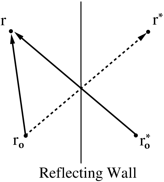
In such a situation, binary collisions modelled by eq.(5) happen on average only between particles at an initial distance $|\vec{r}_{i}j|\cong\sigma$, i.e. at distances much smaller than the radius of curvature of the spherical boundary. In such a situation the boundary can be approximated as a flat wall. Shifting to Cartesian coordinates such that the origin lies on the intersection of $\vec{r}_{ij}$ with boundary and orienting the $y$,$z$ axis tangentially to the surface, the system factorizes in two free Smoluchowsky equations for the $y$,$z$ coordinates and a one dimensional equations for the $x=x_{ij}-\sigma$ coordinate

which can be exactly solved [22] with the image method [18] (fig.2):

.

The whole solution $G_{1}^{wall}$ for a point particle starting in $\vec{r}_{0}$ consists of the superposition in the $x\leq 0$ semi-space of the free Green’s function (2) of a particle in $\vec{r}_{0}=\left(x_{0},y_{0},z_{0}\right)$ and an image particle in $\vec{r}_{0}^{*}=\left(-x_{0},y_{0},z_{0}\right)$. Such a solution can be implemented with just a single operation by extracting the new position $\vec{r}\left(t+\Delta t\right)$ according to (2) and reflecting the $x$ coordinate whenever $x>0$. An event-driven algorithm implementing such scheme is the following:

1. 1.

   extract the random displacements $\Delta x$, $\Delta y$, $\Delta z$,

2. 2.

   define a fictive velocity $v_{x}=\Delta x/\Delta t$

3. 3.

   calculate the fictive collision time $t_{c}:x_{0}+v_{x}t_{c}=0$

4. 4.

   calculate fictive the post-collision velocity $v_{x}^{*}=-v_{x}$

5. 5.

   calculate the final position $x\left(t+\Delta t\right)=x\left(t\right)+v_{x}\cdot t_{c}+v_{x}^{*}\cdot\left(\Delta t-t_{c}\right)$

When mapping back from the Brownian Center of Mass (BCoM) reference system to the original particles’ coordinates, the whole Brownian collision $\vec{r}_{i}\left(t\right)\rightarrow\vec{r}_{i}\left(t+\Delta t\right)$, $\vec{r}_{j}\left(t\right)\rightarrow\vec{r}_{j}\left(t+\Delta t\right)$ follows a procedure strictly recollecting the collision of two classical HSs:

1. 1.

   extract two random displacements $\Delta\vec{r}_{i}$, $\Delta\vec{r}_{j}$ according to (2)

2. 2.

   define two fictive velocities $\vec{v}_{i}=\Delta\vec{r}_{i}/\Delta t$, $\vec{v}_{j}=\Delta\vec{r}_{j}/\Delta t$

3. 3.

   calculate the fictive collision time $t_{c}\in\left[0,\Delta t\right]$, and the normal $\hat{n}^{*}$ between the two spheres at contact at time $t_{c}$

4. 4.

   calculate the fictive post-collision velocities $\vec{v}_{i}^{*}=\vec{v}_{i}-2\left(\hat{n}^{*}\cdot\vec{v}_{ij}\right)\hat{n}^{*}$ and $\vec{v}_{j}^{*}=\vec{v}_{j}+2\left(\hat{n}^{*}\cdot\vec{v}_{ij}\right)\hat{n}^{*}$ with $\vec{v}_{ij}=\vec{v}_{i}-\vec{v}_{j}$

5. 5.

   calculate the final positions $\vec{r}_{i}\left(t+\Delta t\right)=\vec{r}_{i}\left(t\right)+\vec{v}_{i}\cdot t_{c}+\vec{v}_{i}^{*}\cdot\left(\Delta t-t_{c}\right)$ and $\vec{r}_{j}\left(t+\Delta t\right)=\vec{r}_{j}\left(t\right)+\vec{v}_{j}\cdot t_{c}+\vec{v}_{j}^{*}\cdot\left(\Delta t-t_{c}\right)$

Therefore, any event-driven molecular dynamic code [17] can be adapted to simulate the OBD of HSs by extracting at each step $\Delta t$ the velocities of the particles according to independent Gaussian distributions such that $\left\langle\vec{v}_{i}^{2}\right\rangle=2dD\Delta t^{-1}$; a consistency check to perform is to ensure that within the chosen time-step $\Delta t$ less than one collision per particle occurs on average.

In realistic colloidal system there is an inherent polydispersity in particle size; more generally, one could be also interested to mixtures of HSs with different characteristics as in all the studies where crystallization must be avoided. Let us now suppose that our system is composed of HSs of diameters $\sigma_{i}$ subject to overdamped Brownian motion with particle-dependent free diffusion coefficient $D_{i}$, i.e. to noises of amplitude $\langle\vec{\xi}_{i}^{2}\rangle=2dD_{i}$; as usual, trajectories are subject to no-flux boundary constraints $\left|\vec{r}_{i}(t)-\vec{r}_{j}(t)\right|\geq\sigma_{ij}$ where $\sigma_{ij}=\left(\sigma_{i}+\sigma_{j}\right)/2$. Let’s suppose again to fix a time-step $\Delta t$ small enough to consider only binary collisions; for two particles $i$ and $j$ the equations become

.

The first step is to separate equations (7); transformation (4) does not succeed any longer as the transformed noises have a non-zero correlation $D_{i}-D_{j}$. To properly define the “Brownian center of mass” (BCoM), we start from the ansatz $\vec{R}_{CM}=a_{i}\vec{r}_{i}+a_{j}\vec{r}$ and impose zero correlation among the random displacements of the BCoM and the inter-particle distance: $0=\left\langle\Delta\vec{R}_{CM}\Delta\vec{r}_{ij}\right\rangle\propto a_{i}D_{i}-a_{j}D_{j}$; a proper dimensionless choice is $a_{i}=(D_{i}+D_{j})/D_{j}\propto D_{i}^{-1}$.

In the limit of $\Delta t$ small enough such that the $|\vec{r}_{ij}|=\sigma_{ij}$ the boundary can be approximated with a flat hard wall and the zero flux problem can be solved along the dimension perpendicular to the wall (we assume it is the $x$ direction). Let’s again define fictive velocities both in the original reference system and in the BCoM system $v_{\alpha}=\Delta x_{\alpha}/\Delta t$ for $\alpha\in\left\{i,j,CM,ij\right\}$.

The change of coordinates to the BCoM system is

with inverse

In the BOcM system the collision corresponds to imposing the no-flux boundary collision and is simply

and therefore the fictive velocities after the collision are

with collision matrix

This is to be compared with the classical collision matrix for two elastic particles of masses $m_{i}$, $m_{j}$

that has a similar structure if one but with switched indexes $i\leftrightarrow j$ such the role of the mass $m_{i}$ during a collision is played by the inverse diffusivity $D_{i}^{-1}$.

As a check, we consider a fixed particle with $D_{i}=0$; this is equivalent for particle $i$ as having an infinite mass (noise does not move it) and the collision is

as it should be (notice that $v_{j}^{*}=-v_{j}$ as $v_{i}=0$ for $D_{i}=0$); an analogous result comes by sending the “mass” of particle $j$ to zero (i.e. $D_{j}=\infty$).

To summarize, let’s recall that the full event-driven collision scheme for classical particles is

1. 1.

   calculate collision time $t_{c}$ from the “good” root of $\left\|\vec{r}_{ij}+\vec{v}_{ij}t_{c}\right\|=\vec{\sigma}_{ij}$

2. 2.

   bring particles at contact $\vec{r}_{i}=\vec{r}_{i}+\vec{v}_{i}t_{c}$ ,$\vec{r}_{j}=\vec{r}_{j}+\vec{v}_{j}t_{c}$

3. 3.

   let $\vec{\sigma}_{ij}=\vec{r}_{ij}(t_{c})$ , $\hat{\sigma}_{ij}=\vec{\sigma}_{ij}/\left\|\vec{\sigma}_{ij}\right\|$ ,$\mathit{v}_{i}=\vec{v}_{i}\cdot\hat{\sigma}_{ij}$,$\mathit{v}_{j}=\vec{v}_{j}\cdot\hat{\sigma}_{ij}$

4. 4.

   pre-collision: $\left(\begin{array}[]{c}\mathit{v}^{\prime}_{i}\\ \mathit{v}^{\prime}_{j}\end{array}\right)=C_{class}\left(\begin{array}[]{c}\mathit{v}_{i}\\ \mathit{v}_{j}\end{array}\right)$

5. 5.

   collision: $\vec{v}_{i}^{\prime}=\vec{v}_{i}-\mathit{v}{}_{i}\hat{\sigma}_{ij}+\mathit{v}^{\prime}_{i}\hat{\sigma}_{ij}$ , $\vec{v}_{j}^{\prime}=\vec{v}_{j}-\mathit{v}{}_{j}\hat{\sigma}_{ij}+\mathit{v}^{\prime}_{j}\hat{\sigma}_{ij}$

Therefore, to modify an Event Driven code for polydisperse HSs into an Event Driven Brownian Dynamics, simply extract random displacements $\Delta\vec{r}_{i}$ at fixed intervals $t,t+\Delta t,t+2\Delta t,\ldots$, define fictive velocities $\vec{v}_{i}=\Delta\vec{r}_{i}/\Delta t$ and evolve the system for a time $\Delta t$ using for the collision the matrix $C_{Brown}$ instead of $C_{class}$.

Insofar, only system not subject to external forces have been considered. For overdamped Brownian motion, constant forces add constant drifts to the random displacements of the particles. Polydisperse particles are to be expected to experience drifts of different magnitudes even in presence of an homogeneous fields (like gravity or an electrical field). Therefore, the two body equation becomes

where $\vec{g}_{ij}=\vec{g}_{i}-\vec{g}_{j}$ is the difference among the constant drifts of the two particles. Notice that homogeneous drifts do not produce any change in the equations for the inter-particles distances $\vec{r}_{ij}$ as $\vec{g}_{ij}=0$, but just add a constant drift to the BCoM $\vec{R}_{CM}$; therefore, Brownian Event Driven simulations can be implemented extracting particle displacements according to the Green function of the Smoluchowsky equation for a single particle with drift instead of (2).

To see the effects of no-zero $\vec{g}_{ij}$, let’s consider again a $\Delta t$ small enough such that the collision can be approximatively by a flat wall. Factorizing the motion in the directions perpendicular ($x$) and parallel ($y,z$) to the wall, one is left with solving the Smoluchowsky equation with a reflecting boundary in the case of constant drift. This problem has been solved at the beginning of the last century in the seminal paper by M. Smoluchowsky [22] (pp. 569-574; see [14], pp. 2714 for an English version). Assuming that the reflecting boundary is the plane $\partial\Omega=\left\{x=0\right\}$, the evolution of the probability distribution function follows the equation

where $c=-\beta g$, $\beta=1/k_{B}T$ is the inverse temperature and $g$ is a constant force.

Solving for the initial condition $p\left(x,t=0|x_{0}\right)=\delta\left(x-x_{0}\right)$ one obtains the solution

where $erfc\left(z\right)=1-erf\left(z\right)$ is the complementary error function and the error function is $erf(z)=\sqrt{4/\pi}\int_{-\infty}^{z}ds\exp\left[-s^{2}\right]$.

Such a solution is not amenable of a simple geometric implementation in terms of a naive collision mechanism: in this case, for each collision one must transform the coordinates to the BCoM reference system, extract the displacements according to (9) and transform back to the original coordinate system. As a further caveat, high enough constant inter-particle drifts imply the accumulation of particles at short distances (fig.3); the appearance of such inhomogeneous structures is a critical situation is critical for event-driven algorithms as it can produce unacceptable slowing-down of the simulation (via the growth of the number of collision per unit time) and eventually numerical errors [17]. Notice that such issues of non-zero drifts among nearby HSs are often disregarded in the simulations of sheared particles where collisions between hard disks or hard spheres are implemented as elastic collisions of the fictive velocities [23, 8, 13, 12, 15] . Since for HSs structural quantities like the pressure are strictly related to the radial distribution function at contact, a careful analysis of the importance of the drift term in relation to the strength of the noise should be performed to avoid disregarding possible relevant corrections.