Reconstruction of the interaction term between dark matter and dark energy using SNe Ia, BAO, CMB, H(z) and X-ray gas mass fraction

Journal: Journal of Cosmology and Astroparticle physics

Freddy Cueva Solano Ulises Nucamendi Affiliation: Instituto de Física y Matemáticas Affiliation: Universidad Michoacana de San Nicolás de Hidalgo Affiliation: Edificio C-3, Ciudad Universitaria, CP. 58040 Affiliation: Morelia, Michoacán, México Email: freddy@ifm.umich.mx Email: ulises@ifm.umich.mx

Abstract

Recently, in [1] we developed a parametric reconstruction method to a homogeneous, isotropic and spatially flat Friedmann-Robertson-Walker (FRW) cosmological model filled of a fluid of dark energy (DE) with constant equation of state (EOS) parameter interacting with dark matter (DM). The reconstruction method is based on expansions of the general interaction term and the relevant cosmological variables in terms of Chebyshev polynomials which form a complete set orthonormal functions. This interaction term describes an exchange of energy flow between the DE and DM within dark sector. In this article, we reconstruct the interaction function expanding it in terms of only the first four Chebyshev polynomials and obtain the best estimation for the coefficients of the expansion assuming three models: (a) a DE equation of the state parameter $w=-1$ (an interacting cosmological $\Lambda$ ), (b) a DE equation of the state parameter $w=$ constant with a dark matter density parameter fixed, (c) a DE equation of the state parameter $w=$ constant with a free constant dark matter density parameter to be estimated, and using the recent five test data: Union2 SNe Ia data set from “The Supernova Cosmology Project” (SCP) composed by 557 type Ia supernovae, the Baryonic Acoustic Oscillations (BAO), the CMB anisotropies from 7-year WMAP experiment, the Hubble expansion rate data and the X-ray gas mass fraction. In all the cases, the preliminary reconstruction shows that in the best scenario there exist the possibility of a crossing of the noninteracting line $Q=0$ in the recent past within the $1\sigma$ and $2\sigma$ errors from positive values at early times to negative values at late times. This means that, in this reconstruction, there is an energy transfer from DE to DM at early times and an energy transfer from DM to DE at late times. We conclude that this fact is an indication of the possible existence of a crossing behavior in a general interaction coupling between dark components. Finally, we conclude that in this scenario, the observations put strong constraints on the strength of the interaction so that its magnitude can not solve the coincidence problem or at least alleviate significantly.

pacs

95.36.+x, 98.80.-k, 98.80.Es

1 Introduction

Recent observations of the apparent magnitude of Supernova Ia (SNIa) suggest that the universe is in a stage of recent acceleration [2]-[3]. This has now been confirmed by another sets of independent observational data as such the measurements of the galaxy power spectrum and the Baryon Acoustic Oscillations (BAO) detected in the large-scale correlation function of luminous red galaxies in the experiment Sloan Digital Sky Survey (SDSS) [4]-[8], the power spectrum of the cosmic microwave background (CMB) anisotropies measured in the experiment Wilkinson Microwave Anisotropy Probe (WMAP) [9]-[10]. The most simplest explanation to the recent acceleration is the assumption of the existence of a cosmological constant $\Lambda$ assumed to stand for the vacuum density energy ( $\rho_{\Lambda}\approx\Lambda/8\pi G$ ). However, its inferred value from observations $\rho_{\Lambda}^{\rm{obs}}\approx(10^{-12}\rm{Gev})^{4}$ is too tiny when is compared with the theoretical value $\rho_{\Lambda}^{\rm{Pl}}=(10^{18}\rm{Gev})^{4}$ estimated from the application of the quantum field theory to the Planck scale. This is known as the cosmological constant problem [11]-[33]. In addition to this problem, the cosmological constant model has a new one known in the literature as the cosmic coincidence problem [13], [31]-[40] which can be established as: why are both dark densities (dark matter and dark energy) of the same order of magnitude at the present whereas that they were so different in most of the past evolution of the universe?. In order to avoid the problem of fine tuning of the cosmological constant, sometimes it is assumed a null contribution of the vacuum energy density to the cosmological constant which is fixed to zero and therefore it does not contribute to the gravitational sector. In this scenario, we need a different explanation for the present acceleration of the universe. In this direction, it has been proposed a new form of matter-energy named dark energy (DE) which can be a perfect fluid [3], [8], [10], [41]-[42] or a slowly evolving scalar field named quintessence [21]-[40], both with a equation of state (EOS) parameter $w=P_{DE}/\rho_{DE}$ varying with the redshift. In most of the cosmological models considered in the literature, it is generally assumed that dark matter (DM) and DE interact only gravitationally. However, it has been argued that, in the absence of an underlying symmetry suppressing a possible coupling between dark matter and dark energy, a phenomenological interaction between them is not only possible but necessary [43]-[44]. In addition to, it has been speculated that an interaction between dark components is able to alleviate or inclusive to solve the problem of the Cosmic Coincidence [43]-[48]. As a consequence, a large body of work dealing with such a possibility has been explored in the literature [49]-[50].

However, the existence or not of some class of interaction between dark components is to be discerned observationally. To this respect, constraints on the strength of such interaction have been put using different observations [51]-[89].

Recently, it has been suggested that an interacting term $Q(z)$ dependent of the redshift crosses the noninteracting line $Q(z)=0$ [88]-[89]. In [88], this conclusion have been obtained using observational data samples in the range $z\in[0,1.8]$ in order to fit a scenario in which the whole redshift range is divided into a determined numbers of bins and the interaction function is set to be a constant in each bin. They found an oscillatory behavior of the interaction function $Q(z)$ changing its sign several times during the evolution of the universe. On the other hand, in [89] is reported a crossing of the noninteracting line $Q(z)=0$ under the assumption that the interacting term $Q(z)$ is a linearly dependent interacting function of the scale factor with two free parameters to be estimated. They found a crossing from negative values at the past (energy transfers from dark matter to dark energy) to positive values at the present (energy transfers from dark energy to dark matter) at $z\simeq 0.2-0.3$ .

In order to shed light on the question of if an interaction term can solved the The Cosmic Coincidence problem or if in this scenario such crossing really exists, in a previous article [1] we propose the reconstruction of a quite general nongravitational interaction $Q$ between dark components which we introduce phenomenologically in the equations of motion. This reconstruction of $Q$ as a function of the redshift was done in terms of an expansion of Chebyshev Polynomials which constitute a complete orthonormal basis on the finite interval [-1,1] and have the nice property to be the minimax approximating polynomial (this technique has been applied to the reconstruction of the DE potential in [90]-[91]). To this respect, we did the reconstruction of the interaction function using the data from the Union2 Ia Supernova (SNIa) data test (557 data) [3]. In this article, we use a set of data samples covering the wide range of redshift $z\in[0,1089]$ in order to reconstruct the interaction function $Q$ from late to early times.

A summary of the paper is as follows. In the second section, we introduce the general formalism and the equations of motion representing a DE fluid interacting with a DM fluid in Einstein gravity. In the third section, we write the cosmological equations of motion for the interacting dark fluids in a Friedmann-Robertson-Walker (FRW) spacetime. We continue in the section fourth with the introduction and development of the method for reconstructing the interaction function in terms of an expansion in the base of Chebyshev polynomials. The fifth section is dedicated to describe the parametric bayesian statistical method used in the reconstruction of the interaction function together with the chi-square test and the priors used on the free parameters of each model. Additionally, we present the observations used in this article in order to fit the free parameters of the models considered. These observations consist in the data from the Union2 Ia Supernova (SNIa) data test (557 data) [3], the BAO from SDSS DR7 [8], the CMB from 7-year WMAP experiment [10], the Hubble expansion rate (15 data) [93]-[94], [95] and the X-ray gas mass fraction (42 data) [96].

Then, the sixth section is dedicated to the reconstruction of the interaction function and, to put constraints on the parameters of each model and on the coefficients of the Chebyshev expansion Then we give a discussion of the results of the reconstruction and the best estimated values of the parameters of every model fitting the observations. Finally, in the last section we present a brief resume of our principal results and our conclusions.

2 General equations of motion for dark energy interacting with dark matter.

We assume an universe formed by four components: the baryonic matter fluid $(b)$ , the radiation fluid $(r)$ , the dark matter fluid $(DM)$ and the dark energy fluid $(DE)$ . Moreover all these constituents are interacting gravitationally and additionally only the dark components interact nongravitationally through an energy exchange between them mediated by the interaction term defined below.

The gravitational equations of motion are the Einstein field equations

G_{\mu\nu}=8\pi G\left[T^{b}_{\mu\nu}+T^{r}_{\mu\nu}+T^{DM}_{\mu\nu}+T^{DE}_{\mu\nu}\right],

(1)

whereas that the equations of motion for each fluid are

\nabla^{\nu}T^{b}_{\mu\nu}=0,

(2)

\nabla^{\nu}T^{r}_{\mu\nu}=0,

(3)

\nabla^{\nu}T^{DM}_{\mu\nu}=-F_{\mu},

(4)

\nabla^{\nu}T^{DE}_{\mu\nu}=F_{\mu},

(5)

where the respective energy-momentum tensor for the fluid $i$ is defined as $(i=b,r,DM,DE)$ ,

T^{i}_{\mu\nu}=\rho_{i}\,u_{\mu}u_{\nu}+(g_{\mu\nu}+u_{\mu}u_{\nu})P_{i},

(6)

here $u_{\mu}$ is the velocity of the fluids (assumed to be the same for each one) where as $\rho_{i}$ and $P_{i}$ are respectively the density and pressure of the fluid $i$ measured by an observer with velocity $u^{\mu}$ . $F_{\mu}$ is the cuadrivector of interaction between dark components and its form is not known a priori because in general we do not have fundamental theory, in case of existing, to predict its structure. We project the equations (2)-(5) in a part parallel to the velocity $u^{\mu}$ ,

u^{\mu}\nabla^{\nu}T^{b}_{\mu\nu}=0,

(7)

u^{\mu}\nabla^{\nu}T^{r}_{\mu\nu}=0,

(8)

u^{\mu}\nabla^{\nu}T^{DM}_{\mu\nu}=-u^{\mu}F_{\mu},

(9)

u^{\mu}\nabla^{\nu}T^{DE}_{\mu\nu}=u^{\mu}F_{\mu},

(10)

and in other part orthogonal to the velocity using the projector $h_{\beta\mu}=g_{\beta\mu}+u_{\beta}u_{\mu}$ acting on the hypersurface orthogonal to the velocity $u^{\mu}$ ,

h^{\mu\beta}\nabla^{\nu}T^{b}_{\mu\nu}=0,

(11)

h^{\mu\beta}\nabla^{\nu}T^{r}_{\mu\nu}=0,

(12)

h^{\mu\beta}\nabla^{\nu}T^{DM}_{\mu\nu}=-h^{\mu\beta}F_{\mu},

(13)

h^{\mu\beta}\nabla^{\nu}T^{DE}_{\mu\nu}=h^{\mu\beta}F_{\mu},

(14)

using (6) in (7)-(10) we obtain the mass energy conservation equations for each fluid,

u^{\mu}\nabla_{\mu}\rho_{b}+\left(\rho_{b}+P_{b}\right)\nabla_{\mu}u^{\mu}=0,

(15)

u^{\mu}\nabla_{\mu}\rho_{r}+\left(\rho_{r}+P_{r}\right)\nabla_{\mu}u^{\mu}=0,

(16)

u^{\mu}\nabla_{\mu}\rho_{DM}+\left(\rho_{DM}+P_{DM}\right)\nabla_{\mu}u^{\mu}=u^{\mu}F_{\mu},

(17)

u^{\mu}\nabla_{\mu}\rho_{DE}+\left(\rho_{DE}+P_{DE}\right)\nabla_{\mu}u^{\mu}=-u^{\mu}F_{\mu}.

(18)

On the other hand, introducing (6) in (11)-(14) it permits to have the Euler equations for every fluid,

h^{\mu\beta}\nabla_{\mu}P_{b}+\left(\rho_{b}+P_{b}\right)u^{\mu}\nabla_{\mu}u^{\beta}=0,

(19)

h^{\mu\beta}\nabla_{\mu}P_{r}+\left(\rho_{r}+P_{r}\right)u^{\mu}\nabla_{\mu}u^{\beta}=0,

(20)

h^{\mu\beta}\nabla_{\mu}P_{DM}+\left(\rho_{DM}+P_{DM}\right)u^{\mu}\nabla_{\mu}u^{\beta}=-h^{\mu\beta}F_{\mu},

(21)

h^{\mu\beta}\nabla_{\mu}P_{DE}+\left(\rho_{DE}+P_{DE}\right)u^{\mu}\nabla_{\mu}u^{\beta}=h^{\mu\beta}F_{\mu}.

(22)

Finally we closed the system of equations assuming the following state equations for the respectively baryonic, dark matter, radiation components,

$\displaystyle P_{b}$	$\displaystyle=$	$\displaystyle 0,\,$	(23)
$\displaystyle P_{DM}$	$\displaystyle=$	$\displaystyle 0,\,$	(24)
$\displaystyle P_{r}$	$\displaystyle=$	$\displaystyle\frac{1}{3}\,\rho_{r},\,$	(25)

while for the dark energy we assume a state equation with constant parameter $w$ ,

\displaystyle P_{DE}

\displaystyle=

\displaystyle w\rho_{DE}.\,

(26)

3 Cosmological Equations of motion for dark energy interacting with dark matter.

We assumed that the background metric is described by the flat Friedmann-Robertson-Walker (FRW) metric written in comoving coordinates as supported by the anisotropies of the cosmic microwave background (CMB) radiation measured by the WMAP experiment [9]

ds^{2}=-dt^{2}+a^{2}(t)\left(dr^{2}+r^{2}d\Omega^{2}\right),

(27)

where $a(t)$ is the scale factor and $t$ is the cosmic time. In these coordinates we choose for the normalized velocity,

u^{\mu}=(1,0,0,0),

(28)

and therefore we have,

	$\displaystyle\nabla_{\mu}u^{\mu}$	$\displaystyle=$	$\displaystyle 3\,\frac{\dot{a}}{a}\equiv 3H,$		(29)
	$\displaystyle u^{\mu}\nabla_{\mu}u^{\beta}$	$\displaystyle=$	$\displaystyle 0,$		(30)

where $H$ is the Hubble parameter and the point means derivative respect to the cosmic time. In congruence with the symmetries of spatial isotropy and homogeneity of the FRW spacetime, the densities and pressures of the fluids are depending only of the cosmic time, $\rho_{i}(t)$ , $P_{i}(t)$ , and at the same time, the parallel and orthogonal components of the cuadrivector of interaction with respect to the velocity are respectively,

	$\displaystyle u^{\mu}F_{\mu}$	$\displaystyle=$	$\displaystyle Q(a),$		(31)
	$\displaystyle h^{\mu\beta}F_{\mu}$	$\displaystyle=$	$\displaystyle 0,$		(32)

where $Q(a)$ is known as the interaction function depending on the scale factor. The introduction of the state equations (23)-(26), the metric (27) and the expressions (28)-(32) in the equations of mass energy conservation for the fluids (15)-(18) produces,

{\dot{\rho}}_{b}+3H\rho_{b}=0,

(33)

{\dot{\rho}}_{r}+4H\rho_{r}=0,

(34)

{\dot{\rho}}_{DM}+3H\rho_{DM}=Q,

(35)

{\dot{\rho}}_{DE}+3\left(1+w\right)H\rho_{DE}=-Q.

(36)

On the other hand, the Euler equations (19)-(22) are satisfied identically and do not produce any new equation. From the Einstein equation (1) we complete the equations of motion with the first Friedmann equation,

H^{2}\left(a\right)=\frac{8\pi G}{3}\left(\rho_{b}+\rho_{r}+\rho_{DM}+\rho_{DE}\right).

(37)

Its convenient to define the following dimensionless density parameters $\Omega^{\star}_{i}$ , for $i=b,r,DM,DE$ , as the energy densities normalized by the critical density at the actual epoch,

\Omega^{\star}_{i}\equiv\frac{\rho_{i}}{\rho_{crit}^{0}},\\

(38)

and the corresponding dimensionless density parameters at the present,

\Omega^{0}_{i}\equiv\frac{\rho^{0}_{i}}{\rho_{crit}^{0}},\\

(39)

where $\rho_{crit}^{0}\equiv 3H^{2}_{0}/8\pi G$ is the critical density today and $H_{0}$ is the Hubble constant. Solving (33) and (34) in terms of the redshift $z$ , defined as $a=1/(1+z)$ , we obtain the known solutions for the baryonic matter and radiation density parameters respectively:

\Omega^{\star}_{b}(z)=\Omega_{b}^{0}{(1+z)}^{3},\\

(40)

\Omega^{\star}_{r}(z)=\Omega_{r}^{0}{(1+z)}^{4}.\\

(41)

The energy conservation equations (35) and (36) for both dark components are rewritten in terms of the redshift as:

	$\displaystyle\frac{\mathrm{d}{\rho}_{DM}}{\mathrm{d}z}-\frac{3}{1+z}\,\rho_{DM}=-\frac{Q(z)}{(1+z)\cdot H(z)},$		(42)
	$\displaystyle\frac{\mathrm{d}{\rho}_{DE}}{\mathrm{d}z}-\frac{3(1+w)}{1+z}\,\rho_{DE}=\frac{Q(z)}{(1+z)\cdot H(z)}.$		(43)

Phenomenologically, we choose to describe the interaction between the two dark fluids as an exchange of energy at a rate proportional to the Hubble parameter:

\displaystyle Q(z)

\displaystyle\equiv

\displaystyle\rho_{crit}^{0}\cdot(1+z)^{3}\cdot H(z)\cdot{\rm I}_{\rm Q}(z).

(44)

The term $\rho_{crit}^{0}\cdot(1+z)^{3}$ has been introduced by convenience in order to mimic a rate proportional to the behavior of a matter density without interaction. Let be note that the dimensionless interaction function ${\rm I}_{\rm Q}(z)$ depends of the redshift and it will be the function to be reconstructed. With the help of (44), we rewrite the equations for the dark fluids (42)-(43) as,

	$\displaystyle\frac{\mathrm{d}\Omega^{\star}_{DM}}{\mathrm{d}z}-\frac{3}{1+z}\,\Omega^{\star}_{DM}=-(1+z)^{2}\cdot{\rm I}_{\rm Q}(z),$		(45)
	$\displaystyle\frac{\mathrm{d}\Omega^{\star}_{DE}}{\mathrm{d}z}-\frac{3(1+w)}{1+z}\,\Omega^{\star}_{DE}=(1+z)^{2}\cdot{\rm I}_{\rm Q}(z).$		(46)

4 General Reconstruction of the interaction using Chebyshev polynomials.

We do the parametrization of the dimensionless coupling ${\rm I}_{\rm Q}(z)$ in terms of the Chebyshev polynomials, which form a complete set of orthonormal functions on the interval $[-1,1]$ . They also have the property to be the minimax approximating polynomial, which means that has the smallest maximum deviation from the true function at any given order [90]-[91]. Without loss of generality, we can then expand the coupling ${\rm I}_{\rm Q}(z)$ in the redshift representation as:

{\rm I}_{\rm Q}(z)\equiv\sum_{n=0}^{N}\lambda_{n}\cdot T_{n}(z),

(47)

where $T_{n}(z)$ denotes the Chebyshev polynomials of order $n$ with $n\in[0,N]$ and $N$ a positive integer. The coefficients of the polynomial expansion $\lambda_{n}$ are real free dimensionless parameters. Then the interaction function can be rewritten as

Q(z)=\rho_{crit}^{0}\cdot(1+z)^{3}\cdot H(z)\cdot\sum_{n=0}^{N}\lambda_{n}\cdot T_{n}(z).

(48)

We introduce (47) in (45)-(46) and integrate both equations obtaining the solutions,

	$\displaystyle\Omega^{\star}_{DM}(z)$	$\displaystyle=$	$\displaystyle(1+z)^{3}\left[{\Omega_{DM}^{0}}-\frac{z_{max}}{2}\sum_{n=0}^{N}\lambda_{n}\,\cdot K_{n}(x,0)\right],$		(49)
	$\displaystyle\Omega^{\star}_{DE}(z)$	$\displaystyle=$	$\displaystyle(1+z)^{3(1+w)}\left[{\Omega_{DE}^{0}}+\frac{z_{max}}{2}\sum_{n=0}^{N}\lambda_{n}\,\cdot K_{n}(x,w)\right]\,,$		(50)

where we have defined the integrals

\displaystyle K_{n}(x,w)\equiv\int_{-1}^{x}\frac{T_{n}(\tilde{x})}{(a+b\tilde{x})^{(1+3w)}}\,d\tilde{x}\,\,,

(51)

and the quantities,

	$\displaystyle x\equiv\frac{2\,z}{z_{max}}-1,$		(52)
	$\displaystyle a\equiv 1\,+\,\frac{z_{max}}{2},$		(53)
	$\displaystyle b\equiv\frac{z_{max}}{2},$		(54)

here $z_{max}$ is the maximum redshift at which observations are available so that $x\in[-1,1]$ and $|T_{n}(x)|\leq 1$ , for all $n\in[0,N]$ .
Finally, using the solutions (40)-(41) and (49)-(50) we rewrite the Friedmann equation (37) as

H^{2}\left(z\right)=H^{2}_{0}\left[\Omega_{b}^{0}{(1+z)}^{3}+\Omega_{r}^{0}{(1+z)}^{4}+\Omega^{\star}_{DM}(z)+\Omega^{\star}_{DE}(z)\right].

(55)

The Hubble parameter depends of the parameters ( $H_{0}$ , $\Omega_{b}^{0}$ , $\Omega_{r}^{0}$ , $\Omega_{DM}^{0}$ , $\Omega_{DE}^{0}$ , $w$ ) and the dimensionless coefficients $\lambda_{n}$ . However one of the parameters depends of the others due to the Friedmann equation evaluated at the present,

\Omega^{0}_{DE}=1-\Omega_{b}^{0}-\Omega_{r}^{0}-\Omega^{0}_{DM}.

(56)

At the end, for the reconstruction, we have the five parameters ( $H_{0}$ , $\Omega_{b}^{0}$ , $\Omega_{r}^{0}$ , $\Omega_{DM}^{0}$ , $w$ ) and the dimensionless coefficients $\lambda_{n}$ .

To do a general reconstruction in (49)-(50) we must take $N\rightarrow\infty$ and to obtain the solutions in a closed form. The details of the calculation of the integrals $K_{n}(x,w)$ in the right hand side of (49)-(50) are shown in detail in the Appendix A which shows the closed forms (A.9)-(A.10) for the integrals with odd and even integer $n$ subindex, and valid for $w\neq n/3$ , where $n\geq 0$ (see ref. [1]). Finally, we point out the formulas we use for the reconstruction of other important cosmological properties of the universe:

•

The age of the universe at redshift $z$ in [92]:

$\displaystyle t_{0}(z)=\int_{z}^{\infty}\frac{d\tilde{z}}{(1+\tilde{z}).H(\tilde{z})}.$ (57)
•

The deceleration parameter:

$\displaystyle q(z)=-1+\frac{(1+z)}{H(z)}\cdot\frac{dH(z)}{dz}.$ (58)

5 Current observational data and cosmological constraint.

To simplify our analysis, we reconstruct the coupling function ${\rm I}_{\rm Q}(z)$ to different orders ( $N=1,2,3,4$ ), up to order $N=4$ . The details of this reconstruction are described in the Appendix B. (see ref. [1]). In order to do it, we test our cosmological models using the observational data currently available. In this section, we then describe how we use these data.

5.1 Type Ia supernovae.

We test and constrain the coupling function ${\rm I}_{\rm Q}(z)$ using the “Union2” SNe Ia data set from “The Supernova Cosmology Project” (SCP) composed by 557 type Ia supernovae [3]. As it is usual, we use the definition of luminosity distance $d_{L}$ (see ref. [2]) in a flat cosmology,

\displaystyle d_{L}(z,\mathbf{X})

\displaystyle=

\displaystyle c(1+z)\int_{0}^{z}\frac{dz^{\prime}}{H(z^{\prime},\mathbf{X})},

(59)

where $H(z,\mathbf{X})$ is the Hubble parameter, i.e., the expression (55), ” $c$ ” is the speed of light given in units of km/sec and $\mathbf{X}$ represents the parameters of the model,

\displaystyle\mathbf{X}

\displaystyle\equiv

\displaystyle(H_{0},\Omega_{b}^{0},\Omega_{r}^{0},\Omega_{DM}^{0},w,\lambda_{1},...,\lambda_{N}).

(60)

The theoretical distance moduli for the $k$ -th supernova with redshift $z_{k}$ is defined as

\displaystyle\mu^{{\rm th}}(z_{k},\mathbf{X})

\displaystyle\equiv

\displaystyle m(z)-M=5\log_{10}\left[\frac{d_{L}(z_{k},\mathbf{X})}{{\rm Mpc}}\right]+25,

(61)

where $m$ and $M$ are the apparent and absolute magnitudes of the SNe Ia respectively, and the superscript “th” stands for “theoretical”. We construct the statistical $\chi^{2}_{\bf SN}$ function as

\displaystyle\chi^{2}_{\bf SN}(\mathbf{X})

\displaystyle\equiv

\displaystyle\sum_{k=1}^{557}\frac{\left[\mu^{{\rm th}}(z_{k},\mathbf{X})-\mu_{k}\right]^{2}}{\sigma_{k}^{2}},

(62)

where $\mu_{k}$ is the observational distance moduli for the $k$ -th supernova, $\sigma_{k}^{2}$ is the variance of the measurement. With this function $\chi^{2}_{\bf SN}$ , we construct the probability density function (pdf) as

{{\rm{\bf pdf}}}_{\bf SN}(\mathbf{X})={\rm{A}}_{1}\cdot{{\rm e}}^{-\chi^{2}_{\bf SN}(\mathbf{X})\,/2},

(63)

where ${\rm A}_{1}$ is a integration constant.

5.2 Baryon acoustic oscillations

The baryon acoustic oscillations (BAO) are detected in the clustering of the combined 2dFGRS and SDSS main galaxy samples, and measure the distance-redshift relation at $z=0.2$ . Additionally, BAO in the clustering of the SDSS luminous red galaxies measure the distance-redshift relation at $z=0.35$ . The observed scale of the BAO calculated from these samples, as well as from the combined sample, are jointly analyzed using estimates of the correlated errors to constrain the form of the distance measure $D_{v}(z)$ [4]-[7]

D_{v}(z,\mathbf{X})\equiv\left(\left(\int_{0}^{z}\frac{dz^{\prime}}{H(z^{\prime},\mathbf{X})}\right)^{2}\frac{z}{H(z,\mathbf{X})}\right)^{1/3}.

(64)

where $\mathbf{X}$ represents the parameters of the model, see equation (60). The peak position of the BAO depends on the ratio of $D_{v}(z)$ to the sound horizon size at the drag epoch (where baryons were released from photons) $z_{d}$ , which can be obtained by using a fitting formula [4]:

z_{d}=\frac{1291(\Omega_{M})^{-0.419}}{1+0.659(\Omega_{M})^{0.828}}\left[1+b_{1}(\Omega_{b}^{0})^{b_{2}}\right],

(65)

where $\Omega_{M}=\Omega^{0}_{DM}+\Omega_{b}^{0}$ and

	$\displaystyle b_{1}=0.313(\Omega_{M})^{-0.419}\left[1+0.607(\Omega_{M})^{0.674}\right],$		(66)
	$\displaystyle b_{2}=0.238(\Omega_{M})^{0.223}.$		(67)

We use the distance radio $d_{z}$ at $z=0.2$ and $z=0.35$ [4]-[7]

d_{0.2}(\mathbf{X})=\frac{r_{s}(z_{d})}{D_{V}(0.2,\mathbf{X})},\hskip 8.5359ptd_{0.35}(\mathbf{X})=\frac{r_{s}(z_{d})}{D_{V}(0.35,\mathbf{X})},

(68)

where $r_{s}(z_{d},\mathbf{X})$ is the comoving sound horizon size at the baryon drag epoch.

r_{s}(z,\mathbf{X})=\frac{1}{\sqrt{3}}{\int}^{1/(1+z)}_{0}\frac{dz^{\prime}}{H(z^{\prime},\mathbf{X})\sqrt{1+\frac{3\Omega_{b}^{0}}{4(1+z^{\prime})\Omega_{r}^{0}}}}.

(69)

Using the data of BAO of the table 1 and the following inverse covariance matrix of BAO in [7]

The observational $d_{z}$ data
$z$	$d_{z}$
$0.2$	$0.1905\pm 0.0061$
$0.35$	$0.1097\pm 0.0036$

Table 1: Summary of the BAO data set.

C^{-1}_{\bf BAO}=\left(\begin{array}[]{cc}+30124&-17227\\ -17227&+86977\\ \end{array}\right)

(70)

thus, the $\chi^{2}$ function of the BAO data is constructed as:

\chi_{\bf BAO}^{2}(\mathbf{X})=\left(d^{th}_{i}(\mathbf{X})-d^{obs}_{i}\right)^{t}\left(C^{-1}_{\bf BAO}\right)_{ij}\left(d^{th}(\mathbf{X})_{j}-d^{obs}_{j}\right),

(71)

where $(d^{th}-d^{obs})$ is a column vector formed from the values of theory minus the corresponding observational data, with

d^{th}_{i}(\mathbf{X})-d^{obs}_{i}=\left(\begin{array}[]{c}d_{0.20}(\mathbf{X})-0.1905\\ d_{0.35}(\mathbf{X})-0.1097\\ \end{array}\right)

(72)

and ”t“ denotes its transpose. With this $\chi^{2}_{\bf BAO}$ function, we construct the probability density function (pdf) as

{{\rm{\bf pdf}}}_{\bf BAO}(\mathbf{X})={\rm{A}}_{2}\cdot{{\rm e}}^{-\chi^{2}_{\bf BAO}(\mathbf{X})\,/2}

(73)

where ${\rm A}_{2}$ is a integration constant.

5.3 Cosmic microwave background (CMB)

The CMB shift parameter R is provided by [97]

\rm{R}(z_{*},\mathbf{X})\equiv\sqrt{\Omega_{M}H^{2}_{0}}(1+z_{*})(D_{A}(z_{*},\mathbf{X})/c),

(74)

where $\mathbf{X}$ represents the parameters of the model (see equation (60) and the second distance ratio $D_{A}$ is given by:

\displaystyle D_{A}(z_{*},\mathbf{X})=\frac{1}{(1+z_{*})}{\int}^{z_{*}}_{0}\frac{dz^{\prime}}{H(z^{\prime},\mathbf{X})}.

(75)

The redshift $z_{*}$ (the decoupling epoch of photons) is obtained using the fitting function [98]

z_{*}=1048\left[1+0.00124(\Omega^{0}_{b})^{-0.738}\right]\left[1+g_{1}(\Omega_{M})^{g_{2}}\right],

(76)

where $\Omega_{M}=\Omega^{0}_{DM}+\Omega_{b}^{0}$ and the functions $g_{1}$ and $g_{2}$ are

	$\displaystyle g_{1}=\frac{0.0783(\Omega_{b0})^{-0.238}}{1+39.5(\Omega_{b0})^{0.763}},$		(77)
	$\displaystyle g_{2}=\frac{0.560}{1+21.1(\Omega_{b0})^{1.81}}.\,$		(78)

In addition, the acoustic scale $l_{A}$ describes the ratio $D_{A}(z_{*})/r_{s}(z_{*})$ , and is defined as

l_{A}(\mathbf{X})\equiv(1+z_{*})\frac{\pi D_{A}(z_{*},\mathbf{X})}{r_{s}(z_{*},\mathbf{X})},

(79)

where a factor of $(1+z_{*})$ arises because $D_{A}(z_{*},\mathbf{X})$ is the proper angular diameter distance, whereas $r_{s}(z_{*},\mathbf{X})$ is the comoving sound horizon at $z_{*}$ . The fitting formula of $r_{s}(z,\mathbf{X})$ is given by the equation (69). The seven year WMAP observations [10] give the maximum likelihood values according to table 2.

$l_{A}(z_{*})$	$302.40$
$R(z_{*})$	$1.7239$
$z_{*}$	$1090.89$

Table 2: The observational CMB data.

Following [10], the $\chi^{2}$ function for the CMB data is

\chi_{\bf CMB}^{2}(\mathbf{X})=\left(x^{th}_{i}(\mathbf{X})-x^{obs}_{i}\right)^{t}\left(C^{-1}_{\bf CMB}\right)_{ij}\left(x^{th}_{j}(\mathbf{X})-x^{obs}_{j}\right),

(80)

where $(x^{th}-x^{obs})$ is a column vector formed from the values of theory minus the corresponding observational data, with

x^{th}_{i}(\mathbf{X})-x^{obs}_{i}=\left(\begin{array}[]{l}{}_{A}(z_{*})-302.40\\ R(z_{*})-1.7239\\ z_{*}-1090.89\\ \end{array}\right)

(81)

”t“ denotes its transpose and $(C^{-1}_{\bf CMB})_{ij}$ is the inverse covariance matrix. In [10], the inverse covariance matrix is also given as follows

C^{-1}_{\bf CMB}=\left(\begin{array}[]{ccc}+2.3050&+29.6980&-1.3330\\ +29.698&+6825.27&-113.18\\ -1.3330&-113.180&+3.4140\\ \end{array}\right).

(82)

With this function $\chi^{2}_{\bf CMB}$ , we construct the probability density function (pdf) as

{{\rm{\bf pdf}}}_{\bf CMB}(\mathbf{X})={\rm{A}}_{3}\cdot{{\rm e}}^{-\chi^{2}_{\bf CMB}(\mathbf{X})\,/2}

(83)

where ${\rm A}_{3}$ is a integration constant.

5.4 Hubble expansion rate (H)

The Hubble parameter can be written as the following form:

H(z)=-\frac{1}{1+z}\frac{dz}{dt}.

(84)

So,through measuring $dz/dt$ , we can obtain $H(z)$ . In [99], [100] and [90], the authors indicated that it is possible to use absolute ages of passively evolving galaxies to compute values of $dz/dt$ . The galactic spectral data used by [90] come from the Gemini Deep Survey [101] and the archival data [102]-[107]. Detailed calculations of $dz/dt$ can be found in [90]. Simon obtained $H(z)$ in the range of [0,1.8]. The twelve observational Hubble data from [93],[94] are list in the table 3. In addition, in [95], the authors took the BAO scale as a standard ruler in the radial direction, obtain three more additional data: $H(z=0.24)=79.69\pm 2.32$ , $H(z=0.34)=83.80\pm 2.96$ and $H(z=0.43)=86.45\pm 3.27$ (in units of $Km\,s^{-1}Mpc^{-1}$ ).

$z$	$0.0$	$0.1$	$0.17$	$0.27$	$0.4$	$0.48$	$0.88$	$0.90$	$1.30$	$1.43$	$1.53$	$1.73$
$H(z)(Km\,s^{-1}Mpc^{-1})$	$74.2$	$69$	$83$	$77$	$95$	$97$	$90$	$117$	$168$	$177$	$140$	$202$
$1\sigma$	$\pm 3.6$	$\pm 12$	$\pm 8$	$\pm 14$	$\pm 17$	$\pm 60$	$\pm 40$	$\pm 23$	$\pm 17$	$\pm 18$	$\pm 14$	$\pm 40$

Table 3: The observational

H(z)

data.

We can use these data to constraint different kinds of dark energy models and determine the best fit values of the model parameters by minimizing [109]

\displaystyle\chi^{2}_{H}(\mathbf{X})

\displaystyle\equiv

\displaystyle\sum_{i=1}^{15}\frac{\left[H^{{\rm th}}(\mathbf{X},z_{i},)-H^{obs}(z_{i})\right]^{2}}{\sigma^{2}(z_{i})}.

(85)

where $\mathbf{X}$ represents the parameters of the model (see equation (60), $H^{{\rm th}}$ is the theoretical value for the Hubble parameter, $H^{obs}$ is the observed value, $\sigma(z_{i})$ is the standard deviation of the measurement, and the summation is over the 15 observational Hubble data points. This test has already been used to constrain several cosmological models [110]-[123]. With this function $\chi^{2}_{\bf H}$ we construct the probability density function (pdf) as

{{\rm{\bf pdf}}}_{\bf H}(\mathbf{X})={\rm{A}}_{4}\cdot{{\rm e}}^{-\chi^{2}_{\bf H}(\mathbf{X})\,/2}

(86)

where ${\rm A}_{4}$ is a integration constant.

5.5 X-ray gas mass fraction (X-ray)

According to the X-ray cluster gas mass fraction observations, the baryon mass fraction in clusters of galaxies can be used to constrain cosmological parameters. The X-ray cluster gas mass fraction, $f_{gas}$ , is defined as the radio of the X-ray gas mass to the total mass of a cluster, which is a constant and independent of the redshift. In the framework of the $\Lambda CDM$ reference cosmology, the X-ray cluster gas mass fraction is presented as [96]

\displaystyle f_{gas}(z)=\frac{KA\gamma b(z)}{1+s(z)}\left(\frac{\Omega_{b}^{0}}{\Omega_{b}^{0}+\Omega^{0}_{DM}}\right)\left(\frac{D^{\Lambda CDM}_{A}(z,\mathbf{X})}{D_{A}(z,\mathbf{X})}\right)^{1.5}

(87)

where $\mathbf{X}$ represents the parameters of the model. The factor $K$ is used to describe the combined effects of the residual uncertainties, such as the instrumental calibration and certain X-ray modeling issues, and a Gaussian prior for the calibration factor is considered by $K=1.0\pm 0.1$ [96]. The parameter $\gamma$ denotes permissible departures from the assumption of hydrostatic equilibrium, due to non-thermal pressure support; the bias factor $b(z)=b_{0}(1+{\alpha}_{b}Z)$ accounts for uncertainties in the cluster depletion factor; $s(z)=s_{0}(1+{\alpha}_{s}Z)$ accounts for uncertainties of the baryon mass fraction in stars and a Gaussian prior for $s_{0}$ is employed, with $s_{0}=0.16\pm 0.05$ [96] and $A$ is the angular correction factor, which is caused by the change in angle for the current test model $\Theta_{2500}$ in comparison with that of the reference cosmology $\Theta^{\Lambda CDM}_{2500}$ :

\displaystyle A=\left(\frac{\Theta^{\Lambda CDM}_{2500}}{\Theta_{2500}}\right){\eta}\approx\left(\frac{H(z,\mathbf{X})D_{A}(z,\mathbf{X})}{\left[H(z,\mathbf{X})D_{A}(z,\mathbf{X})\right]^{\Lambda CDM}}\right)^{\eta},

(88)

here, the index $\eta$ is the slope of the $f_{gas}(r/r_{2500})$ data within the radius $r_{2500}$ , with the best-fit average value $\eta=0.214\pm 0.022$ [96]. And the proper angular diameter distance $D_{A}(z)$ is given by the equation (75). Following the method in [96] and [124] and adopting the updated 42 observational $f_{gas}$ data in [96], the best fit values of the model parameters for the X-ray cluster gas mass fraction analysis are determined by minimizing,

\displaystyle{{\chi}^{2}}_{X_{ray}}(\mathbf{X})

\displaystyle\equiv

\displaystyle\sum_{i=1}^{42}\frac{\left[\left(f_{gas}\right)^{{\rm th}}(z_{i},\mathbf{X})-\left(f_{gas}(z_{i})\right)^{obs}\right]^{2}}{\sigma^{2}(z_{i})}.

(90)

With this function $\chi^{2}_{\bf X_{ray}}$ , we construct the probability density function (pdf) as

{{\rm{\bf pdf}}}_{\bf X_{ray}}(\mathbf{X})={\rm{A}}_{5}\cdot{{\rm e}}^{-\chi^{2}_{\bf X_{ray}}(\mathbf{X})\,/2}

(91)

where ${\rm A}_{5}$ is a integration constant. We have considered the following values to do the fit

	$\displaystyle K=+1.0,\,\,\gamma=+0.9980,\,\,s_{0}=+0.16,$
	$\displaystyle\alpha_{s}=+0.150,\,\,b_{0}=+0.787,\,\,\alpha_{b}=-0.080.\,$

Therefore, using the equations (63), (73), (83), (86) and (91) we build the total probability density function as

{{\rm{\bf Pdf}}}={{\rm{\bf pdf}}}_{\bf SN}\cdot{{\rm{\bf pdf}}}_{\bf BAO}\cdot{{\rm{\bf pdf}}}_{\bf CMB}\cdot{{\rm{\bf pdf}}}_{\bf H}\cdot{{\rm{\bf pdf}}}_{\bf X_{ray}},

(92)

We can then rewrite the above equation as:

{{\rm{\bf Pdf}}}(\mathbf{X})={\rm{A}}\cdot{{\rm e}}^{-\chi^{2}(\mathbf{X})\,/2},\,

(93)

from here we define the total function $\chi^{2}_{T}$ as,

\displaystyle{{\chi}^{2}}\equiv{{\chi}^{2}}_{\bf SN}+{{\chi}^{2}}_{\bf BAO}+{{\chi}^{2}}_{\bf CMB}+{{\chi}^{2}}_{\bf H}+{{\chi}^{2}}_{X_{\bf ray}}.

(94)

Thus the constraints on cosmological models from a combination of the above discussed observational datasets can be obtained by minimizing the equation (94).

5.6 Priors on the total probability density function (Pdf).

In the models I, II and III shown in the Table 4, we marginalize the parameters $\mathbf{Y}=(H_{0},\Omega_{DM}^{0},\Omega_{b}^{0},\Omega_{r}^{0}$ ) in the pdf (92) choosing priors on them. In order to it, we must compute the following integration,

\displaystyle{{\rm{\bf Pdf}}}(\mathbf{V})=\int^{\infty}_{0}\int^{\infty}_{0}\int^{\infty}_{0}\int^{\infty}_{0}{{\rm{\bf Pdf}}}(\mathbf{X})\,{{\rm{\bf Pdf}}}(\mathbf{Y})\,dH_{0}\,d\Omega_{DM}^{0}\,d\Omega_{b}^{0}\,d\Omega_{r}^{0},

(95)

where $\mathbf{V}=(w,\lambda_{1},...,\lambda_{N})$ represents the nonmarginalized parameters, ${{\rm{\bf Pdf}}}(\mathbf{X})$ is given by (92) and ${{\rm{\bf Pdf}}}(\mathbf{Y})$ is the prior probability distribution function for the parameters ( $H_{0},\Omega_{DM}^{0},\Omega_{b}^{0},\Omega_{r}^{0}$ ) which are chosen as Dirac delta priors around the specific values $\mathbf{\tilde{Y}}=(\tilde{H}_{0},\tilde{\Omega}_{DM}^{0},\tilde{\Omega}_{b}^{0},\tilde{\Omega}_{r}^{0}$ ) measured by some other independent observations,

{{\rm{\bf Pdf}}}(\mathbf{Y})=\delta(H_{0}-\tilde{H}_{0})\cdot\delta(\Omega_{DM}^{0}-\tilde{\Omega}_{DM}^{0})\cdot\delta(\Omega_{b}^{0}-\tilde{\Omega}_{b}^{0})\cdot\delta(\Omega_{r}^{0}-\tilde{\Omega}_{r}^{0}).

(96)

Introducing (96) in ((95) it produces,

{{\rm{\bf Pdf}}}(\mathbf{V})=\rm{A}\cdot{{\rm e}}^{-\tilde{\chi}^{2}(\mathbf{V})\,/2},

(97)

where we have defined a new function $\tilde{\chi}^{2}$ depending only on the parameters $\mathbf{V}=(w,\lambda_{1},...,\lambda_{N})$ as,

\displaystyle\tilde{\chi}^{2}(\mathbf{V})

\displaystyle\equiv

\displaystyle\sum_{k=1}^{n}\frac{\left[\mu^{{\rm th}}(z_{k},\mathbf{V},\mathbf{\tilde{Y}})-\mu_{k}\right]^{2}}{\sigma_{k}^{2}}.

(98)

The specific values chosen for the Dirac delta priors are,

•

$\tilde{H}_{0}=70.4\;({{\rm km}}/{{\rm s}}){{\rm Mpc}}^{-1}$ as suggested by the observations in [10].
•

$\tilde{\Omega}_{DM}^{0}=0.227$ ,
•

$\tilde{\Omega}_{b}^{0}=0.0456$ ,
•

$\tilde{\Omega}_{r}^{0}=8.42095\times 10^{-5}$ .

Once constructed the function $\tilde{\chi}^{2}$ (94), we numerically minimize it to compute the “best estimates” for the free parameters of the model: $\mathbf{V}=(w,\lambda_{1},...,\lambda_{N})$ . The minimum value of the $\tilde{\chi}^{2}$ function gives the best estimated values of $\mathbf{V}$ and measures the goodness-of-fit of the model to data. For the Model IV, we leave too the parameter $\Omega_{DM}^{0}$ free to vary and estimated it from the minimization of the $\tilde{\chi}^{2}$ function. In this case, the parameters to be marginalized are $\mathbf{Y}=(H_{0},\Omega_{b}^{0},\Omega_{r}^{0}$ ). Then, the marginalization will be as,

\displaystyle{{\rm{\bf Pdf}}}(\mathbf{V})=\int^{\infty}_{0}\int^{\infty}_{0}\int^{\infty}_{0}{{\rm{\bf Pdf}}}(\mathbf{X})\,{{\rm{\bf Pdf}}}(\mathbf{Y})\,dH_{0}\,d\Omega_{b}^{0}\,d\Omega_{r}^{0}

(99)

where now $\mathbf{V}=(w,\Omega_{DM}^{0},\lambda_{1},...,\lambda_{N})$ represents the nonmarginalized parameters to be estimated, ${{\rm{\bf Pdf}}}(\mathbf{X})$ is given by (92) and ${{\rm{\bf Pdf}}}(\mathbf{Y})$ is the prior probability distribution function for the parameters ( $H_{0},\Omega_{b}^{0},\Omega_{r}^{0}$ ) which are chosen as Dirac delta priors around the specific values $\mathbf{\tilde{Y}}=(\tilde{H}_{0},\tilde{\Omega}_{b}^{0},\tilde{\Omega}_{r}^{0}$ ) given above. In the models II, III and IV the interaction function ${\rm I}_{\rm Q}(z)$ will be reconstructed up to order $N=4$ in the expansion in terms of Chebyshev polynomials.

Models
Models	$\Omega_{DM}^{0}$	EOS parameter $w$	Interaction function
Model I	0.227 (fixed)	constant	${\rm I}_{\rm Q}(z)\equiv 0$
Model II	0.227 (fixed)	-1	${\rm I}_{\rm Q}(z)\neq 0$
Model III	0.227 (fixed)	constant	${\rm I}_{\rm Q}(z)\neq 0$
Model IV	free parameter	constant	${\rm I}_{\rm Q}(z)\neq 0$

Table 4: Summary of the models studied in this work. In the models II, III and IV the interaction function

{\rm I}_{\rm Q}(z)

will be reconstructed. Additionally, in the model IV the parameter

\Omega_{DM}^{0}

is estimated.

6 Results of the reconstruction of the interaction function.

Now, we present the results of the fit of the models listed in the Table 4 with the “Union2” SNe Ia data set [3], the baryon acoustic oscillation (BAO), the cosmic microwave background (CMB) data from 7-year WMAP, the observational Hubble data and the cluster X-ray gas mass fraction, using the priors described in the Section 5.6. For the noninteracting model I, the only free parameter to be estimated is $\theta=\{w\}$ , whilst for the interacting models II, III and IV the free parameters are $\theta=\{\lambda_{0},...,\lambda_{N}\}$ , $\theta=\{w,\lambda_{0},...,\lambda_{N}\}$ and $\theta=\{w,\Omega_{DM}^{0},\lambda_{0},...,\lambda_{N}\}$ respectively, where $N$ is taking the values $N=1,2,3,4$ . In every case, we obtain the best fitted parameters and the corresponding $\tilde{\chi}^{2}_{min}$ .

Model I: $w=$ constant.
Best estimate for the EOS parameter $w$ .
Errors	$\pm 1\sigma$	$\pm 2\sigma$
$\omega$	${-1.0130}^{+0.0168}_{-0.0163}$	${-1.0130}^{+0.0329}_{-0.0334}$

Table 5: The best estimates of the dark energy EOS parameter

w

for the Model I. It was computed through a Bayesian statistical analysis using SNeIa + BAO + CMB + H + X-ray data sets giving

\tilde{\chi}^{2}_{min}=719.2342

Age of the universe
Model I	$\pm 1\sigma$ (Gyr)	$\pm 2\sigma$ (Gyr)
Age	${15.8679}^{+0.0189}_{-0.0201}$	${15.8679}^{+0.0379}_{-0.0400}$

Table 6: Best estimates for the age of the universe and their errors at

1\sigma

and

2\sigma

for the model I using SNeIa + BAO + CMB + H + X-ray data sets.

Model II: $w=-1$ .
Best estimates for the parameters $\lambda_{n}$ .
$\lambda_{n}$	$N=0$	$N=1$	$N=2$	$N=3$	$N=4$
$\lambda_{0}$	$-1.00\times 10^{-5}$	$-1.0296\times 10^{-5}$	$-1.0108\times 10^{-5}$	$-1.0105\times 10^{-5}$	$-1.0120\times 10^{-5}$
$\lambda_{1}$	$0.0$	$2.0027\times 10^{-4}$	$2.0024\times 10^{-4}$	$2.0014\times 10^{-4}$	$2.0006\times 10^{-4}$
$\lambda_{2}$	$0.0$	$0.0$	$1.9990\times 10^{-6}$	$1.9935\times 10^{-6}$	$1.9918\times 10^{-6}$
$\lambda_{3}$	$0.0$	$0.0$	$0.0$	$1.00\times 10^{-11}$	$1.018\times 10^{-14}$
$\lambda_{4}$	$0.0$	$0.0$	$0.0$	$0.0$	$1.00\times 10^{-16}$
$\tilde{\chi}^{2}_{min}$	$719.8193$	$719.8154$	$719.8134$	$719.8131$	$719.8127$

Table 7: Summary of the best estimates of the dimensionless coefficients

\lambda_{n}

of the polynomial expansion of

{\rm I}_{\rm Q}(z)

for the Model II, corresponding to a interacting dark energy EOS parameter

w=-1

. They were computed through a Bayesian statistical analysis using the SNeIa+BAO+CMB+H+X-ray data sets. The number

N

in the top of every column indicates the maximum number of Chebyshev polynomials used in the expansion of

{\rm I}_{\rm Q}(z)

starting from

N=1

N=4

. From the Figure 4 to Figure 8 show the reconstruction of several cosmological variables using these best fitted values.

Model II: $w=-1$ .
Errors	$\pm 1\sigma$	$\pm 2\sigma$
$\lambda_{0}$	${-1.0108\times 10^{-5}}^{+0.0105\times 10^{-5}}_{-0.0104\times 10^{-5}}$	${-1.0108\times 10^{-5}}^{+0.0282\times 10^{-5}}_{-0.0244\times 10^{-5}}$
$\lambda_{1}$	${+2.0024\times 10^{-4}}^{+0.0253\times 10^{-4}}_{-0.0223\times 10^{-4}}$	${+2.0024\times 10^{-4}}^{+0.0408\times 10^{-4}}_{-0.0335\times 10^{-4}}$
$\lambda_{2}$	${+1.9990\times 10^{-6}}^{+0.0011\times 10^{-6}}_{-0.0017\times 10^{-6}}$	${+1.9990\times 10^{-6}}^{+0.0028\times 10^{-6}}_{-0.0047\times 10^{-6}}$

Table 8: Summary of the

1\sigma

and

2\sigma

errors of the best estimates for

N=2

Age of the universe
Model II	$\pm 1\sigma$ (Gyr)	$\pm 2\sigma$ (Gyr)
Age	$15.85028^{+0.000022}_{-0.000025}$	$15.85028^{+0.000032}_{-0.000039}$

Table 9: Best estimates for the age of the universe and their errors at

1\sigma

and

2\sigma

for the model II using SNeIa + BAO + CMB + H + X-ray data sets.

Refer to caption — Figure 1: Contours correspond to $1\sigma$ , $2\sigma$ confidence levels constrained from joint SNeIa + BAO + CMB + H + X-ray data analysis for the marginalized probability densities of the model II, using an expansion in terms of the first $N=2$ Chebyshev polynomials in the ( $\lambda_{0}$ - $\lambda_{1}$ ) and ( $\lambda_{1}$ - $\lambda_{2}$ ) planes. It is clear that before marginalization, we have three free parameters ( $\lambda_{0}$ , $\lambda_{1}$ , $\lambda_{2}$ ). In every figure, we marginalized on one of the parameters.

Model III: $w=$ constant.
Best estimates for the parameters $\lambda_{n}$ and $w$ .
$\lambda_{n}$	$N=0$	$n=1$	$n=2$	$n=3$	$n=4$
$\lambda_{0}$	$-1.00\times 10^{-5}$	$-1.0040\times 10^{-5}$	$-1.0015\times 10^{-5}$	$-1.0001\times 10^{-5}$	$-1.00\times 10^{-5}$
$\lambda_{1}$	$0.0$	$2.0021\times 10^{-4}$	$2.0040\times 10^{-4}$	$2.0120\times 10^{-4}$	$2.0390\times 10^{-4}$
$\lambda_{2}$	$0.0$	$0.0$	$9.9980\times 10^{-6}$	$9.9970\times 10^{-6}$	$9.9962\times 10^{-6}$
$\lambda_{3}$	$0.0$	$0.0$	$0.0$	$1.0010\times 10^{-9}$	$1.0020\times 10^{-10}$
$\lambda_{4}$	$0.0$	$0.0$	$0.0$	$0.0$	$1.00\times 10^{-12}$
$\omega$	$-1.0089$	$-1.0088$	$-1.0086$	$-1.0089$	$-1.0092$
$\tilde{\chi}^{2}_{min}$	$719.2984$	$719.2861$	$719.1833$	$719.1779$	$719.1731$

Table 10: Summary of the best estimates of the dimensionless coefficients

\lambda_{n}

of the polynomial expansion of

{\rm I}_{\rm Q}(z)

for the Model III, corresponding to a interacting dark energy EOS parameter

w=

constant and

\Omega_{DM}^{0}=0.227

. They were computed through a Bayesian statistical analysis using the SNeIa+BAO+CMB+H+X-ray data sets. The number

N

in the top of every column indicates the maximum number of Chebyshev polynomials used in the expansion of

{\rm I}_{\rm Q}(z)

starting from

N=1

N=4

. From the Figure 4 to Figure 8 show the reconstruction of several cosmological variables using these best fitted values.

Model III: $w=$ constant.
Errors	$\pm 1\sigma$	$\pm 2\sigma$
$\lambda_{0}$	${-1.0015\times 10^{-5}}^{+0.0860\times 10^{-5}}_{-0.0473\times 10^{-5}}$	${-1.0015\times 10^{-5}}^{+0.1000\times 10^{-5}}_{-0.1339\times 10^{-5}}$
$\lambda_{1}$	${+2.0040\times 10^{-4}}^{+0.5885\times 10^{-4}}_{-0.1020\times 10^{-4}}$	${+2.0040\times 10^{-4}}^{+0.8034\times 10^{-4}}_{-0.1813\times 10^{-4}}$
$\lambda_{2}$	${+9.9980\times 10^{-6}}^{+2.0691\times 10^{-6}}_{-0.1588\times 10^{-6}}$	${+9.9980\times 10^{-6}}^{+2.7073\times 10^{-6}}_{-0.3744\times 10^{-6}}$
$\omega$	${-1.0086}^{+0.0041}_{-0.0292}$	${-1.0086}^{+0.0046}_{-0.0312}$

Table 11: Summary of the

1\sigma

and

2\sigma

errors of the best estimates for

N=2

Age of the universe
Model III	$\pm 1\sigma$ (Gyr)	$\pm 2\sigma$ (Gyr)
Age	$15.86064^{+0.0337}_{-0.0054}$	$15.86064^{+0.0360}_{-0.0062}$

Table 12: Best estimates for the age of the universe and their errors at

1\sigma

and

2\sigma

for the model III using SNeIa + BAO + CMB + H + X-ray data sets.

Model IV: $w=$ constant and $\Omega_{DM}^{0}=$ constant
Best estimates for the parameters $\lambda_{n}$ , $w$ and $\Omega_{DM}^{0}$ .
$\lambda_{n}$	$n=0$	$n=1$	$n=2$	$n=3$	$n=4$
$\lambda_{0}$	$-1.00\times 10^{-5}$	$-1.00\times 10^{-5}$	$-1.0010\times 10^{-5}$	$-1.0006\times 10^{-5}$	$-1.0002\times 10^{-5}$
$\lambda_{1}$	$0.0$	$2.0314\times 10^{-4}$	$2.0331\times 10^{-4}$	$2.0385\times 10^{-4}$	$2.0220\times 10^{-4}$
$\lambda_{2}$	$0.0$	$0.0$	$9.9990\times 10^{-6}$	$9.9925\times 10^{-6}$	$9.9915\times 10^{-6}$
$\lambda_{3}$	$0.0$	$0.0$	$0.0$	$1.0068\times 10^{-8}$	$1.0125\times 10^{-10}$
$\lambda_{4}$	$0.0$	$0.0$	$0.0$	$0.0$	$1.00\times 10^{-12}$
$w$	$-1.0089$	$-1.0089$	$-1.0088$	$-1.0088$	$-1.0089$
$\Omega_{DM}^{0}$	$+0.2278$	$+0.2278$	$+0.2278$	$+0.2279$	$+0.2279$
$\tilde{\chi}^{2}_{min}$	$718.6851$	$718.6602$	$718.6236$	$718.5704$	$718.5617$

Table 13: Summary of the best estimates of the dimensionless coefficients

\lambda_{n}

of the polynomial expansion of

{\rm I}_{\rm Q}(z)

for the Model IV, corresponding to a interacting dark energy EOS parameter

w=

constant and

\Omega_{DM}^{0}

as a free parameter to be estimated. They were computed through a Bayesian statistical analysis using the SNeIa+BAO+CMB+H+X-ray data sets. The number

N

in the top of every column indicates the maximum number of Chebyshev polynomials used in the expansion of

{\rm I}_{\rm Q}(z)

starting from

N=1

N=4

. From the Figure 4 to Figure 8 show the reconstruction of several cosmological variables using these best fitted values.

Model IV: $w=$ constant and $\Omega_{DM}^{0}=$ constant.
Errors	$\pm 1\sigma$	$\pm 2\sigma$
$\lambda_{0}$	${-1.0010\times 10^{-5}}^{+0.0616\times 10^{-5}}_{-0.01015\times 10^{-5}}$	${-1.0010\times 10^{-5}}^{+0.1122\times 10^{-5}}_{-0.0434\times 10^{-5}}$
$\lambda_{1}$	${+2.0331\times 10^{-4}}^{+0.0756\times 10^{-4}}_{-0.0173\times 10^{-4}}$	${+2.0331\times 10^{-4}}^{+0.1887\times 10^{-4}}_{-0.0681\times 10^{-4}}$
$\lambda_{2}$	${+9.9990\times 10^{-6}}^{+0.0891\times 10^{-6}}_{-0.0489\times 10^{-6}}$	${+9.9990\times 10^{-6}}^{+0.1550\times 10^{-6}}_{-0.1073\times 10^{-6}}$
$\omega$	${-1.0088}^{+3.9588\times 10^{-8}}_{-0.0658}$	${-1.0088}^{+1.8109\times 10^{-7}}_{-0.0848}$
$\Omega^{0}_{DM}$	${+0.2278}^{+8.0936\times 10^{-5}}_{-0.0056}$	${+0.2278}^{+2.58411\times 10^{-4}}_{-0.0079}$

Table 14: Summary of the

1\sigma

and

2\sigma

errors of the best estimates for

N=2

Age of the universe
Model IV	$\pm 1\sigma$ (Gyr)	$\pm 2\sigma$ (Gyr)
Age	$15.8515^{+0.1409}_{-0.0010}$	$15.8515^{+0.1907}_{-0.0032}$

Table 15: Best estimates for the age of the universe and their errors at

1\sigma

and

2\sigma

for the model IV using SNeIa + BAO + CMB + H + X-ray data sets.

The Figure 4 shows the reconstruction of the dimensionless interaction function ${\rm I}_{\rm Q}(z)$ as a function of the redshift for the models II (corresponding to a dark energy EOS parameter $w=-1$ ), III (corresponding to a dark energy EOS parameter $w=$ constant and $\Omega_{DM}^{0}$ fixed) and IV (corresponding to a dark energy EOS parameter $w=$ constant and $\Omega_{DM}^{0}$ as a free parameter to be estimated) respectively.

The Figure 5 shows the reconstruction of the dark matter and dark energy density parameters $\Omega^{\star}_{DM}(z)$ , $\Omega^{\star}_{DE}(z)$ as a function of the redshift for the models II, III and IV described above.

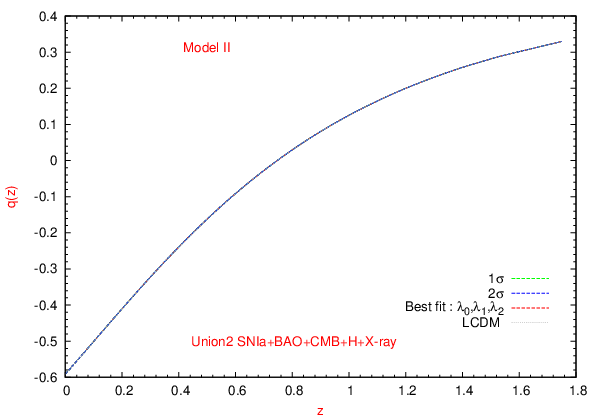
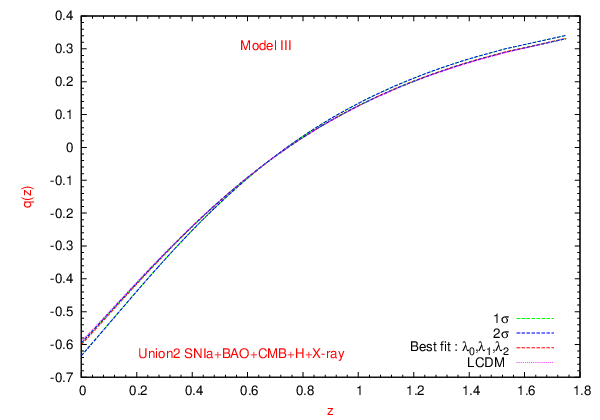
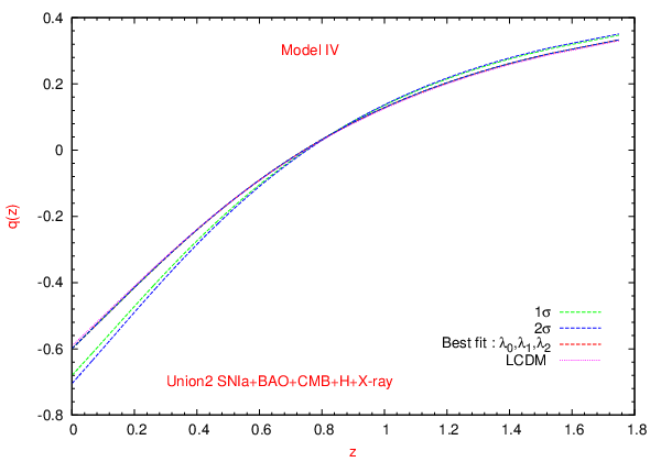
The Figure 6 shows the reconstruction of the deceleration parameter $q(z)$ as a function of the redshift for the models II, III and IV respectively.

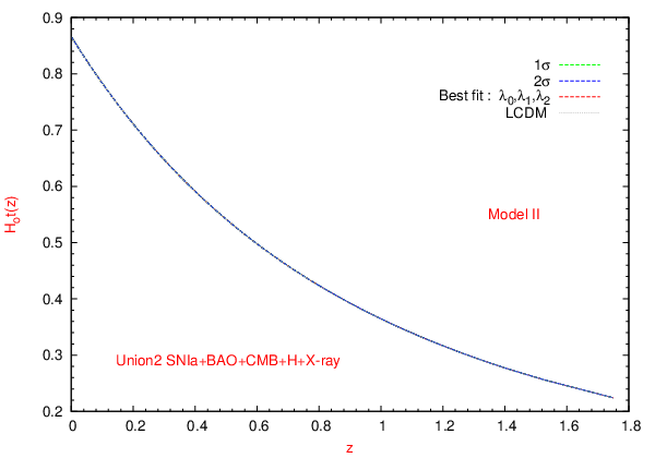
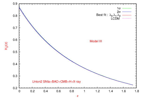
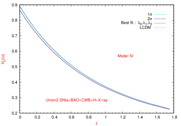
The Figure 7 shows the reconstruction of the age of the universe $H_{0}t(z)$ as a function of the redshift for the models II, III and IV described respectively.

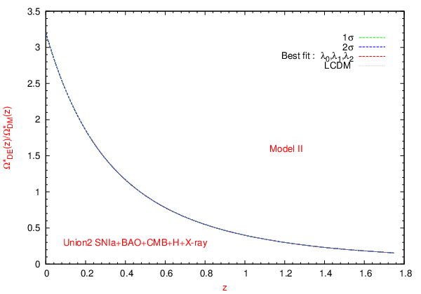
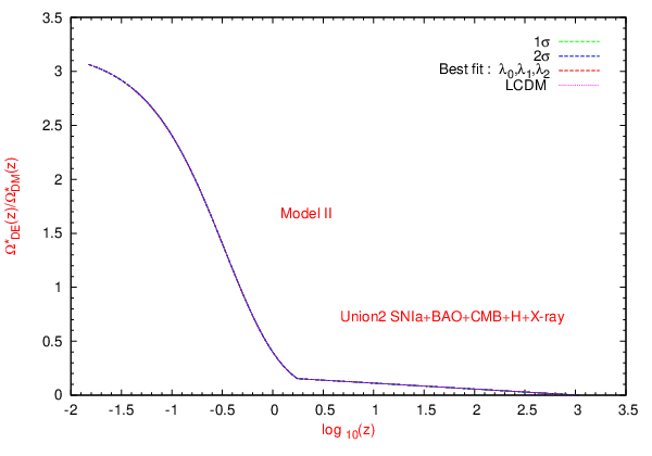
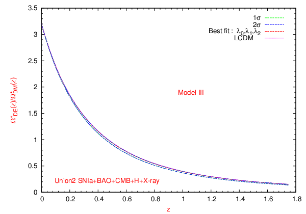
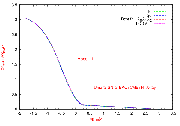
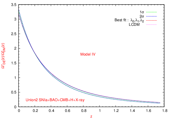
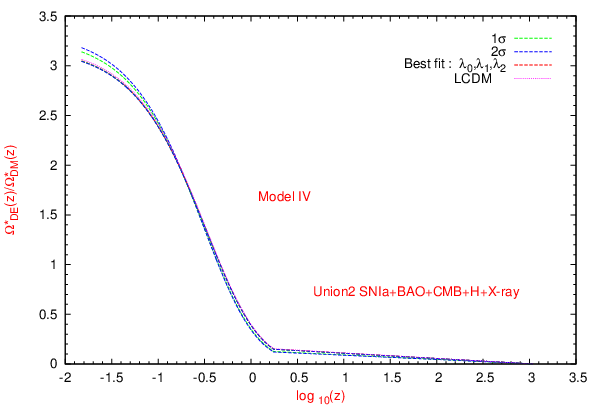
The Figure 8 shows the reconstruction of the rate between dark density parameters $\Omega^{\star}_{DE}(z)/\Omega^{\star}_{DM}(z)$ as a function of the redshift for the models II, III and IV described above.

All these Figures show the superposition of the best estimates for every cosmological variable in terms of the parameters $\lambda_{n}$ corresponding to the coefficients of the polynomial expansion (47) ranging from $N=1$ to $4$ . The Tables 7, 10 and 13, show the best fitted parameters and the minimum of the function $\tilde{\chi}_{min}^{2}$ for the models II, III and IV respectively. From these tables, we can note the fast convergence of the best estimates when the numbers of parameters $N$ is increased in the expansion (47).

The Figure 9 shows the reconstruction of the dimensionless interaction function ${\rm I}_{\rm Q}(z)$ as a function of the redshift, using the best estimates for $N=2$ and their confidence intervals at $1\sigma$ and $2\sigma$ for the models II (corresponding to a dark energy EOS parameter $w=-1$ ), III (corresponding to a dark energy EOS parameter $w=$ constant and $\Omega_{DM}^{0}$ fixed) and IV (corresponding to a dark energy EOS parameter $w=$ constant and $\Omega_{DM}^{0}$ as a free parameter to be estimated) respectively.

The Figure 10 shows the reconstruction of the dark matter and dark energy density parameters $\Omega^{\star}_{DM}(z)$ , $\Omega^{\star}_{DE}(z)$ as a function of the redshift, using the best estimates for $N=2$ and their confidence intervals at $1\sigma$ and $2\sigma$ for the models II, III and IV described above.

The Figure 11 which shows the reconstruction and the behavior of the deceleration parameter $q(z)$ as a function of the redshift and their confidence intervals at $1\sigma$ and $2\sigma$ for the models II, III and IV respectively.

The Figure 12 shows the reconstruction of the age of the universe $H_{0}t(z)$ as a function of the redshift and their confidence intervals at $1\sigma$ and $2\sigma$ for the models II, III and IV already described respectively.

The Figure 13 shows the reconstruction of the rate between dark density parameters $\Omega^{\star}_{DE}(z)/\Omega^{\star}_{DM}(z)$ as a function of the redshift and their confidence intervals at $1\sigma$ and $2\sigma$ for the models II, III and IV already mentioned.

These last Figures show the superposition of the best estimates for every cosmological variable and their confidence intervals at $1\sigma$ and $2\sigma$ . The Tables 8, 11 and 14, show the best fitted parameters with their respective $1\sigma$ and $2\sigma$ .

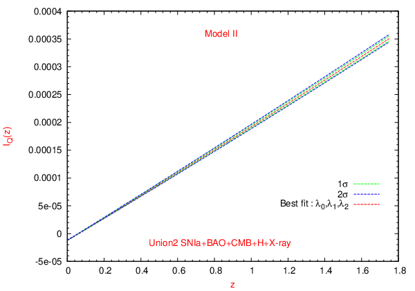
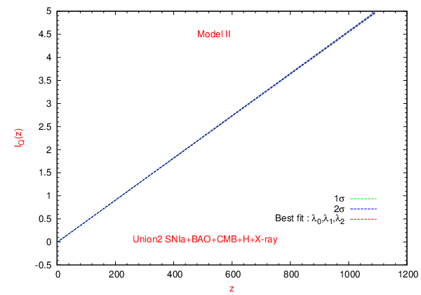
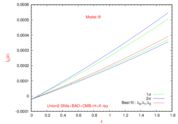
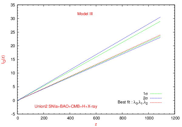
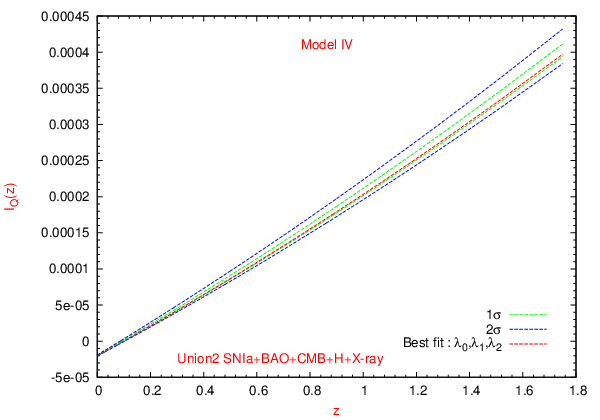
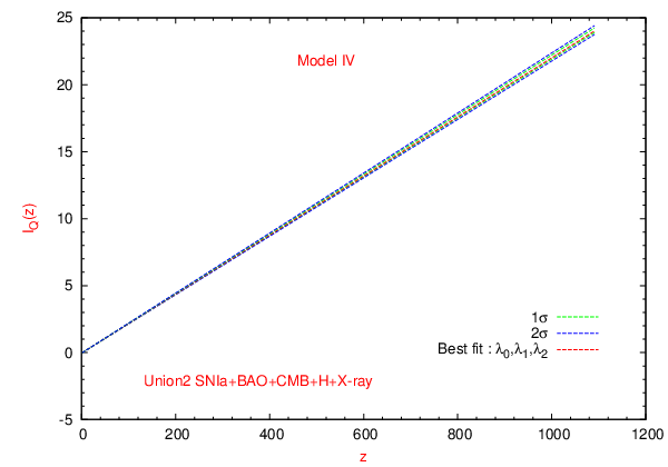
From Figures 4 to 9 we notice that, for all interacting models, the best estimates for the interaction function ${\rm I}_{\rm Q}(z)$ cross marginally the noninteracting line ${\rm I}_{\rm Q}(z)=0$ during the present cosmological evolution (at around $z\approx 0.09$ ) changing sign from positive values at the past (energy transfers from dark energy to dark matter) to negative values at the present (energy transfers from dark matter to dark energy). However, taking in account the errors corresponding to the fit using three parameters ( $N=2$ ), we see that within the $1\sigma$ and $2\sigma$ errors, it exists the possibility of crossing of the noninteracting line in the recent past at around the range $z\in(0.08,0.12)$ . Crossings of the noninteracting line $Q(z)=0$ have been recently reported at the references [88] (with an interacting term $Q(z)$ proportional to the Hubble parameter) and [1]. The direction of the change found in our work is in the same direction to the results published by these references where a crossing (from positive values at the past to negative values at the present was found at $z\simeq 0-0.12$ . On the other hand, we did not find the oscillatory behavior of the interaction function found by Cai and Su [88] who, using observational data samples in the range $z\in[0,1.8]$ , fitted a scheme in which the whole redshift range is divided into a determined numbers of bins and the interaction function set to be a constant in each bin.

From Figures 5 to Figures 10 show that, for all the interacting models studied in this work, the best estimates for the dark energy density parameter $\Omega^{\star}_{DE}(z)$ become to be definite positive at all the range of redshifts considered in the data samples. However, this statement is conclusive because within the $1\sigma$ and $2\sigma$ errors for the fit with three parameters ( $N=2$ ), the $\Omega^{\star}_{DE}(z)$ becomes to be positive in all the range of redshifts considered (remember that we are using five data sets and then the space parameters permitted is remarkably reduced). According to the Model 4, note also that the behavior of dark matter $\Omega^{\star}_{DM}(z)$ density parameter, for $1\sigma$ and $2\sigma$ errors exist the possibility of being smaller compared to the noninteracting model (LCDM model).

From Figures 6 to Figure 11, show that, for all models, a transition from a deceleration era at early times dominated by the dark and baryonic matter density to an acceleration era at late times corresponding to the present domain of the dark energy density. This transition deceleration-acceleration to take place at redshift at around $z\approx 0.7$ (it was also obtained by [129]), while that the rhythm of current universe at around $q_{0}\approx 0.6$ . It is clear for our constraint, that the universe tends to an early time to accelerate and a milder expansion rhythm at present.

We can see from the figure 5 to 10 that, at the present, the dark energy density parameter becomes $\Omega^{0}_{DE}(z)\approx 0.7$ , which is sufficiently large to generate a non negligible dimensionless interacting term of the order of ${\rm I}^{0}_{\rm Q}\approx-10^{-5}$ , as is shown in the Figures 4 and 9. In fact, in these same figures we can appreciate that in the interval of redshifts $z\in[0,1090.89]$ , the dimensionless interaction is in the range ${\rm I}_{\rm Q}\in[-10^{-5},50]$ for the Model II, ${\rm I}_{\rm Q}\in[-10^{-5},35]$ for the Model III and ${\rm I}_{\rm Q}\in[-10^{-5},25]$ for the Model IV respectively, corresponding at $2\sigma$ error. The order of magnitude of this interaction is in agreement with the local constraints put on the strength of a constant dimensionless interaction derived from the fit to a data sample of virial masses of relaxed galaxies clusters obtained using weak lensing, x-ray and optical data [127].

On the contrary, a recent study fitting CMB anisotropy data from the seven-year Wilkinson Microwave Anisotropy Probe (WMAP) [10], the BAO distance measurements [7], the Constitution sample of SnIa [2] and constraints on the present-day Hubble constant, put stronger constraints on the magnitude of such dimensionless strength of the order of $\xi\approx 10^{-2}-10^{-4}$ [128].

Another important aspect concerns to study the coincidence problem, then from the Figures 5 and 10, we note that the Models II and III, do not have the possibility of alleviating this problem. Their behaviors are in a degree similar to the LCDM model. On the contrary, our Model IV, has the possibility of alleviating it at $2\sigma$ error. In the behavior of dark matter $\Omega^{\star}_{DM}(z)$ density parameter, within $1\sigma$ and $2\sigma$ errors, exist the possibility of being smaller compared to the corresponding noninteracting model (LCDM model).

It is interesting to note that from the Figure 7 to Figure 12 and according to the results of the tables 9, 12 and 15, the best fitted values predicted for our models are consistent with the requirement that the universe be older that any of its constituents at a given redshift [102], [92].

From all our analysis, and from the Figure 2 and 3, 5 and 10, show that the $1\sigma$ and $2\sigma$ constraints on the EOS parameter $w$ contain high probability of being in the phantom region, but our results are even consistent and compatible with the LCDM model at $1\sigma$ error.

In general when more cosmic observational data sets are added to constrain our model parameters space, the degeneracies between model parameters will be broken. The reason comes from the fact that the constraints on our models are more stringent that the results obtained in reference [1].

7 Conclusions.

In this paper, we developed theoretically a novel method for the reconstruction of the interaction function between dark matter and dark energy assuming an expansion of the general interaction term proportional to the Hubble parameter in terms of Chebyshev polynomials which form a complete set of orthonormal functions. To show how the method works, we applied it to the reconstruction of the interaction function expanding it in terms of only the first $N$ Chebyshev polynomials (with $N=1,2,3,4$ ) and fitted for the coefficients of the expansion assuming three models: (a) a DE equation of the state parameter $\omega=-1$ (an interacting cosmological $\Lambda$ ), (b) a DE equation of the state parameter $\omega=$ constant and (c) a DE equation of the state parameter $\omega=$ constant and $\Omega_{DM}=$ constant, respectively. The fit of the free parameters of every model is done using the Union2 SNe Ia data set from “The Supernova Cosmology Project” (SCP) composed by 557 type Ia supernovae [3], the Baryon Acoustic Oscillation (BAO), the Cosmic Microwave Background (CMB) data from 7-year WMAP, the Observational Hubble data and the Cluster X-ray Gas Mass Fraction.

Our principal results can be summarized as follows:

1.

Compared with the results of reference [1], our fitting results show a faster convergence of the best fitted values for the several cosmological variables considered in this paper when the numbers of parameters $N$ is increased in the expansion (47).
2.

The best estimates for the interaction function ${\rm I}_{\rm Q}(z)$ prefer to cross the noninteracting line ${\rm I}_{\rm Q}(z)=0$ during the present cosmological evolution. This conclusion is independent of the numbers of coefficients (up to $N=4$ in this work) used in the expansion of ${\rm I}_{\rm Q}(z)$ . The crossing implies a change of sign of ${\rm I}_{\rm Q}(z)$ from positive values at the past (energy transfers from dark energy to dark matter) to negative values at the present (energy transfers from dark matter to dark energy). This direction of decay is similar to the results found in the recent literature [1] and is in disagreement with the oscillatory behavior reported in [88].
3.

The statement above is conclusive because the existence of crossing of the noninteracting line ${\rm I}_{\rm Q}(z)=0$ in some moment of the recent past is totally contained inside the $1\sigma$ and $2\sigma$ constraints given by current observations.
4.

We can state that is reasonable to expect that DE and DM interact via a small but calculable coupling and to be consistent with the observations at $2\sigma$ error. In this aspect, The the Cosmic Microwave Background (CMB) data provides a stringent constraints on the coupling.
5.

We confirm that adding the Baryon Acoustic Oscillation (BAO), the Cosmic Microwave Background (CMB), the Observational Hubble (H) and the Cluster X-ray Gas Mass Fraction (X-ray) data sets, generally reduces the allowed range of the model parameters. It is to say are strongly reduced compared with the results of the ref [1], which were obtained using only Union2 SNe Ia data.
6.

For all the interacting models studied in this work, the best estimates for the dark energy density parameter $\Omega^{\star}_{DE}(z)$ becomes positive definite in the range of redshifts considered in this work. This statement is conclusive because, within the $1\sigma$ and $2\sigma$ errors for the fit with three parameters ( $N=2$ ), $\Omega^{\star}_{DE}(z)$ becomes positive in all the range of redshifts considered in the observational data sets.
7.

The $1\sigma$ and $2\sigma$ confidence intervals, for the EOS parameter $\omega$ considered in the marginalized models III and IV, preferred to be in the phantom region ( $w<-1$ ). But exists a small probability for the EOS parameter $\omega$ of being in the quintessence region. This conclusion is consistent and is within of LCDM model.
8.

According to the Figures 6 and 11 and to our results, we confirm that there is strong evidence that the universe is accelerated in the recent past, which is consistent with studies in [125], [126].
9.

we therefore conclude that our models are consistent with the properties of the cosmological variables and its results are also consistent with the LCDM model at $2\sigma$ error.

Finally, we emphasize the importance of more accurate and extensive measurements. These observations will certainly provide a complementary tool to test the reality of the current cosmological parameters, of the term of interaction between dark sectors and the existence of the crossing of the noninteracting ${\rm I}_{\rm Q}(z)=0$ line and place stringent constraints on them, and as a consequence, to distinguish among the many alternatives models. We believe that the analysis, combined with the results give us the possibility of understanding all that. With the successful experience achieved to reconstruct the general interaction term between dark matter and dark energy, our next step is to extend our study to do a double reconstruction as much the interaction term ${\rm I}_{\rm Q}(z)$ as dark energy equation of state parameter $\omega$ simultaneously, within the dark sectors. More efforts will be required on this way to carry out it.

8 Acknowledgements.

This work was in part supported by grants SNI-20733, CIC-UMSNH No.4.8, UMSNH-CA-22. F. Cueva thanks support by CONACYT-SEP.

References.

References

[1] F. Cueva Solano and U. Nucamendi, Reconstruction of the interaction term between dark matter and dark energy using SNe Ia, JCAP 04 (2012) 011.
[2] SUPERNOVA SEARCH TEAM collaboration, A.G. Riess et al., Observational evidence from supernovae for an accelerating universe and a cosmological constant, Astron. J. 116 (1998) 1009 [astro-ph/9805201] [SPIRES];
SUPERNOVA COSMOLOGY PROJECT collaboration, S. Perlmutter et al., Measurements of $\Omega$ and $\Lambda$ from 42 high-redshift supernovae, Astrophys. J. 517 (1999) 565 [astro-ph/9812133] [SPIRES];
SUPERNOVA SEARCH TEAM collaboration, J.L. Tonry et al., Cosmological results from high-z supernovae, Astrophys. J. 594 (2003) 1 [astro-ph/0305008] [SPIRES];
SUPERNOVA SEARCH TEAM collaboration, A.G. Riess et al., Type Ia supernova discoveries at $z>1$ from the Hubble space telescope: evidence for past deceleration and constraints on dark energy evolution, Astrophys. J. 607 (2004) 665 [astro-ph/0402512] [SPIRES];
SNLS collaboration, P. Astier et al., The supernova legacy survey: measurement of $\Omega_{M}$ , $\Lambda$ and w from the first year data set, Astron. Astrophys. 447 (2006) 31 [astro-ph/0510447] [SPIRES];
A.G. Riess et al., New Hubble space telescope discoveries of type Ia supernovae at $z>1$ : narrowing constraints on the early behavior of dark energy, Astrophys. J. 659 (2007) 98 [astro-ph/0611572] [SPIRES];
T.M. Davis et al., Scrutinizing exotic cosmological models using ESSENCE supernova data combined with other cosmological probes, Astrophys. J. 666 (2007) 716 [astro-ph/0701510] [SPIRES];
ESSENCE collaboration, W.M. Wood-Vasey et al., Observational constraints on the nature of the dark energy: first cosmological results from the ESSENCE supernova survey, Astrophys. J. 666 (2007) 694 [astro-ph/0701041] [SPIRES];
M. Kowalski et al., Improved cosmological constraints from new, old and combined supernova datasets, Astrophys. J. 686 (2008) 749 [arXiv:0804.4142] [SPIRES].
[3] R. Amanullah et al., Spectra and light curves of six type Ia supernovae at $0.511<z<1.12$ and the Union2 compilation, Astrophys. J. 716 (2010) 712 [arXiv:1004.1711] [SPIRES].
[4] SDSS collaboration, D. J. Eisenstein et al., Detection of the baryon acoustic peak in the large-scale correlation function of SDSS luminous red galaxies, Astrophys. J. 633 (2005) 560 [astro-ph/0501171] [SPIRES].
D. J. Eisenstein, W. Hu, Baryon Features in the Matter Transfer Function, Astrophys. J. 496 (1998) 605 [astro-ph/9709112] [SPIRES].
[5] SDSS collaboration, M. Tegmark et al., Cosmological parameters from SDSS and WMAP, Phys. Rev. D 69 (2004) 103501 [astro-ph/0310723] [SPIRES].
SDSS collaboration, M. Tegmark et al., Cosmological Constraints from the SDSS Luminous Red Galaxies, Phys. Rev. D 74 (2006) 123507 [astro-ph/0608632] [SPIRES].
[6] SDSS collaboration, K. Abazajian et al., The First data release of the Sloan Digital Sky Survey, Astron. J. 126 (2003) 2081 [astro-ph/0305492] [SPIRES].
SDSS collaboration, K. Abazajian et al., The Second data release of the Sloan digital sky survey, Astron. J. 128 (2004) 502 [astro-ph/0403325] [SPIRES].
SDSS collaboration, K. Abazajian et al., The Third Data Release of the Sloan Digital Sky Survey, Astron. J. 129 (2005) 1755 [astro-ph/0410239] [SPIRES].
SDSS collaboration, K. Abazajian et al., The Seventh Data Release of the Sloan Digital Sky Survey, Astrophys. J. Suppl. 182 (2009) 543 [astro-ph/0812.0649] [SPIRES].
[7] W. J. Percival et al., Measuring the Baryon Acoustic Oscillations using the Sloan Digital Sky Survey and 2dFGRS, Mon. Not. Roy. Astron. Soc. 381 (2007) 1053 [arXiv: 0705.3323] [SPIRES].
SDSS collaboration, W. J. Percival et al., Baryon Acoustic Oscillations in the Sloan Digital Sky Survey Data Release 7 Galaxy Sample, Mon. Not. Roy. Astron. Soc. 401 (2010) 2148 [astro-ph.CO/0907.1660] [SPIRES].
[8] SDSS collaboration, B. A. Reid et al., Cosmological Constraints from the Clustering of the Sloan Digital Sky Survey DR7 Luminous Red Galaxies, Mon. Not. Roy. Astron. Soc. 404 (2010) 60 [astro-ph.CO/0907.1659] [SPIRES].
[9] WMAP collaboration, C.L. Bennett et al., First year Wilkinson Microwave Anisotropy Probe (WMAP) observations: preliminary maps and basic results, Astrophys. J. Suppl. 148 (2003) 1 [astro-ph/0302207] [SPIRES];
WMAP collaboration, D.N. Spergel et al., First year Wilkinson Microwave Anisotropy Probe (WMAP) observations: Determination of cosmological parameters, Astrophys. J. Suppl. 148 (2003) 175 [astro-ph/0302209] [SPIRES];
WMAP collaboration, D.N. Spergel et al., Wilkinson Microwave Anisotropy Probe (WMAP) three year results: implications for cosmology, Astrophys. J. Suppl. 170 (2007) 377 [astro-ph/0603449][SPIRES].
WMAP collaboration, G. Hinshaw et al., Five-year Wilkinson Microwave Anisotropy Probe (WMAP) observations: data processing, sky maps, basic results, Astrophys. J. Suppl. 180 (2009) 225 [arXiv:0803.0732] [SPIRES].
WMAP collaboration, E. Komatsu et al., Five-Year Wilkinson Microwave Anisotropy Probe (WMAP) Observations: Cosmological Interpretation, Astrophys. J. Suppl. 180 (2009) 330 [arXiv:0803.0547] [SPIRES].
[10] WMAP collaboration, E. Komatsu et al., Seven-Year Wilkinson Microwave Anisotropy Probe (WMAP) observations: Cosmological interpretation, Astrophys. J. Suppl. 192 (2011) 18 [arXiv:1001.4538] [SPIRES].
[11] S. Weinberg,The Cosmological Constant Problem, Rev. Mod. Phys. 61 (1989) 1.
[12] S. M. Carroll, W. H. Press and E. L. Turner, The Cosmological constant, Ann. Rev. Astron. Astrophys. 30 (1992) 499.
[13] P. J. Steinhardt, Cosmological Challenges for the 21th century, in Critical Problems in Physics, V. L. Fitch and D. R. Marlow eds., Princeton University Press, Princeton U.S.A. (1997), pg. 123.
[14] S. Weinberg, Likely values of the cosmological constant, Astrophys. J. 492 (1998) 29 [astro-ph/9701099].
[15] V. Sahni and A. A. Starobinsky, The Case for a positive cosmological Lambda term, Int. J. Mod. Phys. D 9 (2000) 373 [astro-ph/9904398].
[16] S. Weinberg, A Priori probability distribution of the cosmological constant, Phys. Rev. D 61 (2000) 103505 [astro-ph/0002387].
[17] S. M. Carroll, The Cosmological constant, Living Rev. Rel. 4 (2001) 1 [astro-ph/0004075].
[18] T. Padmanabhan, Cosmological constant: The Weight of the vacuum, Phys. Rept. 380 (2003) 235 [hep-th/0212290].
[19] V. Sahni, The Cosmological constant problem and quintessence, Class. Quant. Grav. 19 (2002) 3435 [astro-ph/0202076].
[20] P. J. E. Peebles and B. Ratra, The Cosmological constant and dark energy, Rev. Mod. Phys. 75 (2003) 559 [astro-ph/0207347].
[21] P. J. E. Peebles and B. Ratra, Cosmology with a Time Variable Cosmological Constant, Astrophys. J. 325 (1988) L17.
[22] B. Ratra and P. J. E. Peebles, Cosmological Consequences of a Rolling Homogeneous Scalar Field, Phys. Rev. D 37 (1988) 3406.
[23] B. Ratra and P. J. E. Peebles, Inflation in an open universe, Phys. Rev. D 52 (1995) 1837.
[24] S. M. Carroll, Quintessence and the rest of the world, Phys. Rev. Lett. 81 (1998) 3067 [astro-ph/9806099].
[25] R. R. Caldwell, R. Dave and P. J. Steinhardt, Quintessential cosmology: Novel models of cosmological structure formation, Astrophys. Space Sci. 261 (1998) 303.
[26] J. Zlatev, L.-M. Wang and P. J. Steinhardt, Quintessence, cosmic coincidence, and the cosmological constant, Phys. Rev. Lett. 82 (1999) 896 [astro-ph/9807002].
[27] N. A. Bahcall, J. P. Ostriker, S. Perlmutter, P. J. Steinhardt, The Cosmic triangle: Assessing the state of the universe, Science 284 (1999) 1481 [astro-ph/9906463].
[28] P. J. Steinhardt, L.-M. Wang and I. Zlatev, Cosmological tracking solutions, Phys. Rev. D 59 (1999) 123504 [astro-ph/9812313].
[29] L.-M. Wang, R. R. Caldwell, J. P. Ostriker and P. J. Steinhardt, Cosmic concordance and quintessence, Astrophys. J. 530 (2000) 17 [astro-ph/9901388].
[30] L. P. Chimento, A. S. Jakubi and D. Pavon, Enlarged quintessence cosmology, Phys. Rev. D 62 (2000) 063508 [astro-ph/0005070].
[31] V. Sahni, The Cosmological constant problem and quintessence, Class. Quant. Grav. 19 (2002) 3435 [astro-ph/0202076].
[32] P. S. Corasaniti and E. J. Copeland, Constraining the quintessence equation of state with SnIa data and CMB peaks, Phys. Rev. D 65 (2002) 043004 [astro-ph/0107378].
[33] P. J. E. Peebles and B. Ratra, The Cosmological constant and dark energy, Rev. Mod. Phys. 75 (2003) 559 [astro-ph/0207347].
[34] P. J. Steinhardt, A quintessential introduction to dark energy, Phil. Trans. Roy. Soc. Lond. A 361 (2003) 2497.
[35] P. S. Corasaniti and E. J. Copeland, A Model independent approach to the dark energy equation of state, Phys. Rev. D 67 (2003) 063521 [astro-ph/0205544].
[36] V. Sahni, Dark matter and dark energy, Lect. Notes Phys. 653 (2004) 141 [astro-ph/0403324].
[37] U. Alam, V. Sahni and A. A. Starobinsky, The Case for dynamical dark energy revisited, JCAP 06 (2004) 008 [astro-ph/0403687].
[38] P. S. Corasaniti, M. Kunz, D. Parkinson, E. J. Copeland and B. A. Bassett, The Foundations of observing dark energy dynamics with the Wilkinson Microwave Anisotropy Probe, Phys. Rev. D 70 (2004) 083006 [astro-ph/0406608].
[39] M. Li, X.-D. Li, S. Wang and Y. Wang, Dark Energy, Commun. Theor. Phys. 56 (2011) 525 [astro-ph.CO/1103.5870].
[40] E. J. Copeland, M. Sami and S. Tsujikawa, Dynamics of dark energy, Int. J. Mod. Phys. D 15 (2006) 1753 [hep-th/0603057].
[41] A. Vikhlinin et al., Chandra Cluster Cosmology Project III: Cosmological Parameter Constraints, Astrophys. J. 692 (2009) 1060 [astro-ph/0812.2720].
[42] E. Rozo et al., Cosmological Constraints from the SDSS maxBCG Cluster Catalog, Astrophys. J. 708 (2010) 645 [astro-ph.CO/0902.3702].
[43] S. Campo, R. Herrera and D. Pavon, Toward a solution of the coincidence problem, Phys. Rev. D 78 (2008) 021302(R) [astro-ph/0806.2116].
[44] S. Campo, R. Herrera and D. Pavon, Interacting models may be key to solve the cosmic coincidence, JCAP 01 (2009) 020 [gr-qc/0812.2210].
[45] L. Amendola, Coupled quintessence, Phys. Rev. D 62 (2000) 043511 [astro-ph/9908023] [SPIRES].
[46] L. Amendola and C. Quercellini, Tracking and coupled dark energy as seen by WMAP, Phys. Rev. D 68 (2003) 023514 [astro-ph/0303228] [SPIRES].
[47] L. Amendola, S. Tsujikawa and M. Sami, Phantom damping of matter perturbations, Phys. Lett. B 632 (2006) 155 [astro-ph/0506222] [SPIRES].
[48] G. Olivares, F. Atrio-Barandela and D. Pavon,Matter density perturbations in interacting quintessence models, Phys. Rev. D 74 (2006) 043521 [astro-ph/0607604].
[49] L. Amendola, Coupled quintessence, Phys. Rev. D 62 (2000) 043511 [astro-ph/9908023] [SPIRES]; L. Amendola, Perturbations in a coupled scalar field cosmology, Mon. Not. Roy. Astron. Soc. 312 (2000) 521 [astro-ph/9906073] [SPIRES]; A. P. Billyard and A. A. Coley,Interactions in scalar field cosmology, Phys. Rev. D 61 (2000) 083503 [astro-ph/9908224]; W. Zimdahl, D. Pavon and L. P. Chimento Interacting quintessence, Phys. Lett. B 521 (2001) 133 [astro-ph/0105479]; L. Amendola and C. Quercellini, Tracking and coupled dark energy as seen by WMAP, Phys. Rev. D 68 (2003) 023514 [astro-ph/0303228] [SPIRES]; L. P. Chimento, A. S. Jakubi, D. Pavon and W. Zimdahl, Interacting quintessence solution to the coincidence problem, Phys. Rev. D 67 (2003) 083513 [astro-ph/0303145]; L. Amendola, Linear and non-linear perturbations in dark energy models, Phys. Rev. D 69 (2004) 103524 [astro-ph/0311175]; G. R. Farrar and P. J. E. Peebles, Interacting dark matter and dark energy, Astrophys. J. 604 (2004) 1 [astro-ph/0307316];
[50] S. Campo, R. Herrera and D. Pavon, Soft coincidence in late acceleration, Phys. Rev. D 71 (2005) 123529 [astro-ph/0506482]; Z.-K. Guo, R.-G. Cai and Y.-Z. Zhang, Cosmological evolution of interacting phantom energy with dark matter, JCAP 05 (2005) 002 [astro-ph/0412624]; W. Zimdahl, Interacting dark energy and cosmological equations of state, Int. J. Mod. Phys. D 14 (2005) 2319 [gr-qc/0505056]; S. Campo, R. Herrera, G. Olivares and D. Pavon, Interacting models of soft coincidence, Phys. Rev. D 74 (2006) 023501 [astro-ph/0606520]; G. Huey and B. D. Wandelt, Interacting quintessence. The Coincidence problem and cosmic acceleration, Phys. Rev. D 74 (2006) 023519 [astro-ph/0407196]; L. P. Chimento and D. Pavon, Dual interacting cosmologies and late accelerated expansion, Phys. Rev. D 73 (2006) 063511 [gr-qc/0505096]; M. S. Berger and H. Shojaei, Interacting dark energy and the cosmic coincidence problem, Phys. Rev. D 73 (2006) 083528 [gr-qc/0601086]; M. S. Berger and H. Shojaei, An Interacting Dark Energy Model for the Expansion History of the Universe, Phys. Rev. D 74 (2006) 043530 [astro-ph/0606408]; J. F. Jesus, R. C. Santos, J. S. Alcaniz and J. A. S. Lima, New coupled quintessence cosmology, Phys. Rev. D 78 (2008) 063514 [astro-ph/0806.1366]; J. Valiviita, E. Majerotto and R. Maartens, Instability in interacting dark energy and dark matter fluids, JCAP 07 (2008) 020 [astro-ph/0804.0232]; M. Quartin, M. O. Calvao, S. E. Joras, R. R. R. Reis and I. Waga, Dark Interactions and Cosmological Fine-Tuning, JCAP 05 (2008) 007 [astro-ph/0802.0546]; L. P. Chimento, M. I. Forte, G. M. Kremer, Cosmological model with interactions in the dark sector, Gen. Rel. Grav. 41 (2009) 1125 [astro-ph/0711.2646]; E. Majerotto, J. Valiviita and R. Maartens, Adiabatic initial conditions for perturbations in interacting dark energy models, Mon. Not. Roy. Astron. Soc. 402 (2010) 2344 [astro-ph.CO/0907.4981]; J. C. Fabris, B. Fraga, N. Pinto-Neto and W. Zimdahl, Transient cosmic acceleration from interacting fluids, JCAP 04 (2010) 008 [astro-ph.CO/0910.3246]; S. Z. W. Lip, Interacting Cosmological Fluids and the Coincidence Problem, Phys. Rev. D 83 (2011) 023528 [gr-qc/1009.4942].
[51] L. Amendola, C. Quercellini, D. T. Valentini and A. Pasqui, Constraints on the interaction and selfinteraction of dark energy from cosmic microwave background, Astrophys. J. 583 (2003) L53 [astro-ph/0205097].
[52] L. Amendola, M. Gasperini and F. Piazza, Fitting type Ia supernovae with coupled dark energy, JCAP 09 (2004) 014 [astro-ph/0407573].
[53] D. Pavon, S. Sen and W. Zimdahl, CMB constraints on interacting cosmological models, JCAP 05 (2004) 009 [astro-ph/0402067].
[54] G. Olivares, F. Atrio-Barandela and D. Pavon,Observational constraints on interacting quintessence models, Phys. Rev. D 71 (2005) 063523 [astro-ph/0503242].
[55] R. G. Cai and A. Wang, Cosmology with interaction between phantom dark energy and dark matter and the coincidence problem, JCAP 03 (2005) 002 [hep-th/0411025].
[56] B. Wang, Y. G. Gong and E. Abdalla, Transition of the dark energy equation of state in an interacting holographic dark energy model, Phys. Lett. B 624 (2005) 141 [hep-th/0506069] [SPIRES].
[57] B. Wang, C. Y. Lin and E. Abdalla, Constraints on the interacting holographic dark energy model, Phys. Lett. B 637 (2006) 357 [hep-th/0509107] [SPIRES].
[58] S. Lee, G.-C. Liu and K.-W. Ng, Constraints on the coupled quintessence from cosmic microwave background anisotropy and matter power spectrum, Phys. Rev. D 73 (2006) 083516 [astro-ph/0601333].
[59] R. Mainini and S. Bonometto, Limits on coupling between dark components, JCAP 06 (2007) 020 [astro-ph/0703303].
[60] Z.-K. Guo, N. Ohta and S. Tsujikawa, Probing the Coupling between Dark Components of the Universe, Phys. Rev. D 76 (2007) 023508 [astro-ph/0702015].
[61] B. Wang, J. Zang, C. Y. Lin, E. Abdalla and S. Micheletti, Interacting Dark Energy and Dark Matter: Observational Constraints from Cosmological Parameters, Nucl. Phys. B 778 (2007) 69 [astro-ph/0607126] [SPIRES].
[62] L. Amendola, G. C. Campos and R. Rosenfeld, Consequences of dark matter-dark energy interaction on cosmological parameters derived from SNIa data, Phys.Rev., D 75 (2007) 083506 [astro-ph/0610806] [SPIRES].
[63] O. Bertolami, F. G. Pedro and M. Le Delliou, Dark Energy-Dark Matter Interaction and the Violation of the Equivalence Principle from the Abell Cluster A586, Phys. Lett. B 654 (2007) 165 [astro-ph/0703462].
[64] O. Bertolami, F. G. Pedro and M. Le Delliou, Dark Energy-Dark Matter Interaction from the Abell Cluster A586, [astro-ph/0801.0201].
[65] G. Olivares, F. Atrio-Barandela and D. Pavon,Dynamics of Interacting Quintessence Models: Observational Constraints, Phys. Rev. D 77 (2008) 063513 [astro-ph/0706.3860].
[66] Q. Wu, Y. Gong, A. Wang and J. S. Alcaniz, Current constraints on interacting holographic dark energy, Phys. Lett. B 659(2008) 34 [astro-ph/0705.1006].
[67] C. Feng, B. Wang, E. Abdalla and R.-K. Su, Observational constraints on the dark energy and dark matter mutual coupling, Phys. Lett. B 665 (2008) 111 [astro-ph/0804.0110] [SPIRES].
[68] J.-H. He and B. Wang, Effects of the interaction between dark energy and dark matter on cosmological parameters, JCAP 06 (2008) 010 [astro-ph/0801.4233].
[69] R. Bean, E. E. Flanagan, I. Laszlo and M. Trodden, Constraining Interactions in Cosmology’s Dark Sector, Phys. Rev. D 78 (2008) 123514 [astro-ph/0808.1105].
[70] B. M. Schäfer, The integrated Sachs-Wolfe effect in cosmologies with coupled dark matter and dark energy, Mon. Not. Roy. Astron. Soc. 388 (2008) 1403 [astro-ph/0803.2239].
[71] O. Bertolami, F. G. Pedro and M. Le Delliou, The Abell Cluster A586 and the Equivalence Principle, Gen. Rel. Grav. 41 (2009) 2839 [astro-ph/0705.3118].
[72] J.-Q. Xia, Constraint on coupled dark energy models from observations, Phys. Rev. D 80 (2009) 103514 [astro-ph.CO/0911.4820].
[73] J.-H. He, B. Wang and P. Zhang, Imprint of the interaction between dark sectors in large scale cosmic microwave background anisotropies, Phys. Rev. D 80 (2009) 063530 [gr-qc/0906.0677].
[74] J.-H. He, B. Wang and Y. P. Jing, Effects of dark sectors’ mutual interaction on the growth of structures, JCAP 07 (2009) 030 [gr-qc/0902.0660].
[75] K. Koyama, R. Maartens and Y. S. Song, Velocities as a probe of dark sector interactions, JCAP 10 (2009) 017 [astro-ph.CO/0907.2126].
[76] J. Valiviita, R. Maartens and E. Majerotto, Observational constraints on an interacting dark energy model, Mon. Not. Roy. Astron. Soc. 402 (2010) 2355 [astro-ph.CO/0907.4987].
[77] G. Izquierdo and D. Pavon, Limits on the parameters of the equation of state for interacting dark energy, Phys. Lett. B 688 (2010) 115 [astro-ph.CO/1004.2360].
[78] E. Abdalla, L. R. Abramo and J. C. C. de Souza, Signature of the interaction between dark energy and dark matter in observations, Phys. Rev. D 82 (2010) 023508 [gr-qc/0910.5236] [SPIRES].
[79] J.-H. He, B. Wang, E. Abdalla and D. Pavon, The Imprint of the interaction between dark sectors in galaxy clusters, JCAP 12 (2010) 022 [gr-qc/1001.0079].
[80] S. Cao and N. Liang, Testing the phenomenological interacting dark energy with observational H(z) data, [astro-ph.CO/1012.4879].
[81] L. Lopez Honorez, B. A. Reid, O. Mena, L. Verde and R. Jimenez, Coupled dark matter-dark energy in light of near Universe observations, JCAP 09 (2010) 029 [astro-ph.CO/1006.0877]
[82] M. Martinelli, L. Lopez Honorez, A. Melchiorri and O. Mena, Future CMB cosmological constraints in a dark coupled universe, Phys.Rev. D 81 (2010) 103534 [astro-ph.CO/1004.2410].
[83] F. De Bernardis, M. Martinelli, A. Melchiorri, O. Mena and A. Cooray, Future weak lensing constraints in a dark coupled universe, Phys. Rev. D 84 (2011) 023504 [astro-ph.CO/1104.0652].
[84] O. Bertolami, F. G. Pedro and M. Le Delliou, Testing the interaction of dark energy to dark matter through the analysis of virial relaxation of clusters Abell Clusters A586 and A1689 using realistic density profiles, [astro-ph.CO/1105.3033].
[85] J. He, B. Wang and E. Abdalla, Testing the interaction between dark energy and dark matter via latest observations, Phys. Rev. D 83 (2011) 063515 [astro-ph.CO/1012.3904] [SPIRES].
[86] X.-D. Xu, J.-H. He and B. Wang, Breaking parameter degeneracy in interacting dark energy models from observations, Phys. Lett. B 701 (2011) 513 [astro-ph.CO/1103.2632].
[87] S. Cao, N. Liang and Z.-H. Zhu, Interaction between dark energy and dark matter: observational constraints from H(z), BAO, CMB and SNe Ia, [astro-ph.CO/1105.6274].
[88] R. G. Cai and Q. Su, On the Dark Sector Interactions, Phys. Rev. D 81 (2010) 103514 [astro-ph.CO/0912.1943] [SPIRES].
[89] Y.-H. Li and X. Zhang, Running coupling: Does the coupling between dark energy and dark matter change sign during the cosmological evolution?, Eur. Phys. J. C 71 (2011) 1700 [astro-ph.CO/1103.3185] [SPIRES].
[90] J. Simon, L. Verde and R. Jimenez, Constraints on the redshift dependence of the dark energy potential, Phys. Rev. D 71 (2005) 123001 [astro-ph/0412269] [SPIRES].
[91] E. F. Martinez and L. Verde, Prospects in Constraining the Dark Energy Potential, JCAP 08 (2008) 023 [astro-ph/0806.1871].
[92] T. D. Saini, S. Raychaudhury, V. Sahni and A. A. Starobinsky, Reconstructing the Cosmic Equation of State from Supernova distance, Phys. Rev. Lett. 85 (2000) 6.
[93] A. G. Riess et al., A Redetermination of the Hubble Constant with the Hubble Space Telescope from a Differential Distance Ladder, Astrophys. J. 699 (2009) 539 [astro-ph.CO/0905.0695].
[94] D. Stern, R. Jimenez, L. Verde, M. Kamionkowski and S. A. Stanford, Cosmic Chronometers: Constraining the Equation of State of Dark Energy. I: H(z) Measurements, JCAP 02 (2010) 008 [astro-ph.CO/0907.3149].
[95] E. Gaztanaga, A. Cabre and L. Hui, Clustering of Luminous Red Galaxies IV: Baryon Acoustic Peak in the Line-of-Sight Direction and a Direct Measurement of H(z), Mon. Not. Roy. Astron. Soc. 399 (2009) 1663 [astro-ph/0807.3551].
[96] S. W. Allen, D. A. Rapetti, R. W. Schmidt, H. Ebeling, G. Morris and A. C. Fabian, Improved constraints on dark energy from Chandra X-ray observations of the largest relaxed galaxy clusters, Mon. Not. Roy. Astron. Soc. 383 (2008) 879 [astro-ph/0706.0033].
[97] J. R. Bond, G. Efstathiou and M. Tegmark, Forecasting Cosmic parameter Error from Microwave Background Anisotropy Experiments, Mon. Not. Roy. Astron. Soc. 291 (1997) L33 [astro-ph/9702100][SPIRES].
[98] W. Hu and N. Sugiyama, Small scale cosmological perturbations: An Analytic approach, Astrophys. J. 471 (1996) 542 [astro-ph/9510117][SPIRES].
[99] R. Jimenez and A. Loeb,Constraining cosmological parameters based on relative galaxy ages, Astrophys. J. 573 (2002) 37 [astro-ph/0106145] [SPIRES].
[100] R. Jimenez,L. Verde, T. Treu and D.Stern,Constraining on the equation of state of dark energy and the Hubble constant from stellar ages and the CMB, Astrophys. J. 593 (2003) 622 [astro-ph/0302560] [SPIRES].
[101] R. G. Abraham et al., The Gemini Deep Survey. 1. Introduction to the survey, catalogs and composite spectra, Astron. J. 127 (2004) 2455 [astro-ph/0402436] [SPIRES].
[102] J. Dunlop et al., A. 3.5-Gyr-old galaxy at redshift 1.55, Nature. 381 (1996) 581 [SPIRES].
[103] H. Spinrad et al., LBDS 53w091: an old red galaxy at z=1.552, Astrophys. J. 484 (1997) 581 [astro-ph/9702233] [SPIRES].
[104] T. Treu, M. Stiavelli, S. Casertano, P. Moller and G. Bertin, The properties of field elliptical galaxies at intermediate redshift. I: empirical scaling laws, Mon. Not. Roy. Astron. Soc. 308 (1999) 1037 [astro-ph/9904327][SPIRES].
[105] T. Treu, M. Stiavell, P. Moller, S. Casertano and G. Bertin, The properties of field elliptical galaxies at intermediate redshift. 2: photometry and spectroscopy of an HST selected sample, Mon. Not. Roy. Astron. Soc. 326 (2001) 221 [astro-ph/0104177][SPIRES].
[106] T. Treu, M. Stiavelli, S. Casertano, P. Moller and G. Bertin, The evolution of field early-type galaxies to z 0.7, Astrophys. J. 564 (2002) L13 [astro-ph/0111504][SPIRES].
[107] L. A. Nolan, J. S. Dunlop, R. Jimenez and A. F. Heavens, F stars, metallicity and the ages of red galaxies at z¿1, Mon. Not. Roy. Astron. Soc. 341 (2003) 464 [astro-ph/0103450][SPIRES].
[108] D. Stern, R. Jimenez, L. Verde, S. A. Stanford ans M. Kamionkowski, Cosmic Chronometers: Constraining the Equation of State of Dark Energy. II. A Spectroscopic Catalog of Red Galaxies in Galaxy Clusters, Astrophys. J. Suppl. 188 (2010) 280 [astro-ph.CO/0907.3152].
[109] R. Lazkoz and E. Majerotto, Cosmological constraints combining H(z), CMB shift and SNIa observational data, JCAP 07 (2007) 015 [arXiv: 0704.2606][SPIRES]. J. Lu, L. Xu, M. Liu and Y. Gui, Constraints on accelerating universe using ESSENCE and Gold supernovae data combined with other cosmological probes, Eur. Phys. J. C 58 (2008) 311 [arXiv: 0812.3209][SPIRES].
L. Samushia and B. Ratra, Cosmological Constraints from Hubble Parameter versus Redshift Data, Astrophys. J. 650 (2006) L5 [astro-ph/0607301][SPIRES].
[110] Z. L. Yi and T. J. Zhang, Constraints on holographic dark energy models using the differential ages of passively evolving galaxies, Mod. Phys. Lett. A 22 (2007) 41 [astro-ph/0605596][SPIRES].
[111] H. Lin et al., Observational H(z) data as a complementary to other cosmological probes, Mod. Phys. Lett. A 24 (2009) 1699 [arXiv: 0804.3135][SPIRES].
[112] L. Samushia and B. Ratra, Cosmological constraints from Hubble parameters versus redshift data, Astrophys. J. 650 (2006) L5 [astro-ph/0607301][SPIRES].
[113] H. Wei and S. N. Zhang, Observational H(z) data and cosmological models, Phys. Lett. B 644 (2007) 7 [astro-ph/0609597][SPIRES].
[114] J. F. Zhang, X. Zhang and H. Y. Liu, Holographic dark energy in a cyclic universe, Eur. Phys. J. C 52 (2007) 693 [arXiv: 0708.3121][SPIRES].
[115] H. Wei and S. N. Zhang, Age problem in the holographic dark energy model, Phys. Rev. D 76 (2007) 063003 [arXiv: 0707.2129][SPIRES].
[116] A. Giri, B. Mawlong and R. Mohanta, Determining the CKM angle gamma with B(c) decays, Phys. Rev. D 75 (2007) 097304 [hep-ph/0611212][SPIRES].
[117] M. Dantas, J. S. Alcaniz, D. Jain and A. Dev, Dark energy constraints from Gemini Deep Survey, Astron. Astrophys. 467 (2007) 421 [astro-ph/0607060][SPIRES].
[118] H. Zhang and Z. H. Zhu, Natural pnantom dark energy wiggling Hubble parameter H(z) and direct H(z) data, JCAP. 03 (2008) 007 [astro-ph/0703245][SPIRES].
[119] P. X. Wu and H. W. Yu, Generalized Chaplyging gas model: constraints from Hubble parameter versus redshift data, Phys. Lett. B 644 (2007) 16 [agr-qc/0612055][SPIRES].
[120] L. Feng and Y. P. Yang, Observational constraints on the early dark energy model, Res. Astron. Astrophys. 11 (2011) 751.
[121] H. Wei and S. N. Zhang, Observational H(z) data and cosmological models, Phys. Lett. B 644 (2007) 7 [astro-ph/0609597][SPIRES].
[122] J. B. Lu, Y. X. Gui and L. X. Xu, Observational constraint on generalized Chaplyging gas model, Eur. Phys. J. C 63 (2009) 349 [arXiv: 1004.3365][SPIRES].
[123] L. X. Xu and J. B. Lu, cosmological constraints on generalized Chaplyging gas model: Markov chain Monte Carlo approach, JCAP. 03 (2010) 025 [arXiv: 1002.3344][SPIRES].
[124] S. Nesseris and L. Perivolaropoulos, Crossing the Phantom Divide: Theoretical Implications and Observational Status, JCAP. 01 (2007) 018 [astro-ph/0610092][SPIRES].
[125] C. A. Shapiro and M. S. Turner, What Do We Really Know about Cosmic Acceleration?, Astrophys. J. 649 (2006) 563.
[126] Y. G. Gong, and A. Wang, Observational constraints of the acceleration of the universe, Phys. Rev. D 73 (2006) 083506.
[127] E. Abdalla, L. R. Abramo and J. C. C. de Souza, Signature of the interaction between dark energy and dark matter in observations, Phys. Rev. D 82 (2010) 023508 [gr-qc/0910.5236] [SPIRES].
[128] J. He, B. Wang and E. Abdalla, Testing the interaction between dark energy and dark matter via latest observations, Phys. Rev. D 83 (2011) 063515 [astro-ph.CO/1012.3904] [SPIRES].
[129] S. Campo, R. Herrera, G. Olivares and D. Pavon, Interacting models of soft coincidence, Phys. Rev. D 74 (2006) 023501 [astro-ph/0606520].