Mathematical properties of a semi-classical signal analysis method: noisy signal case
Abstract
Recently, a new signal analysis method based on a semi-classical approach has been proposed [1]. The main idea in this method is to interpret a signal as a potential of a Schrodinger operator and then to use the discrete spectrum of this operator to analyze the signal. In this paper, we are interested in a mathematical analysis of this method in discrete case considering noisy signals.
I INTRODUCTION
Recently, a new signal analysis method based on a semi-classical approach has been proposed [1]. We refer to this method SCSA for Semi-Classical Signal Analysis. The main idea in the SCSA is to interpret a signal as a potential of a Schrodinger operator depending on a semi-classical parameter [2]. It is well-known that if the potential is in the Faddeev class [3], then it can be expressed using a sum of the squared eigenfunctions associated to the negative eigenvalues characterizing the discrete spectrum of the Schrodinger operator and an integral involving the continuous spectrum. Similarly to the other standard approximation methods, by truncating the expression of the potential, the sum part is taken as an estimate of the potential. The proposed estimate depends on the semi-classical parameter. It has been shown that by reducing this parameter the estimation of the signal by the SCSA can be improved [1].
Promising results have been obtained when applying the SCSA to arterial blood pressure. More than a satisfactory estimation of the pressure signals, this method introduced new spectral parameters that seem to contain important physiological information [4, 5]. Moreover, a recent study has shown that the SCSA parameters could be useful in the estimation of some physical parameters related to turbomachinery features [6]. It has been also confirmed by some tests that the SCSA method is robust with respect to corrupting noises. Hence, it can be considered as a filter. However, the mathematical analysis of the SCSA in discrete noisy case has not been considered yet, comparing to other signal analysis methods (see, e.g., [7, 8, 9, 10, 11]),
We propose in this paper to study the mathematical properties of the SCSA in discrete case considering noisy signals. We propose also to study how to choose an appropriate semi-classical parameter to analyze a signal. In Section II, we recall the methodology and some mathematical properties of the SCSA method in the continuous case. Then, we study this method in discrete case in Section III. In Section IV, the SCSA method is studied in discrete noisy case. An a-posteriori error bound of the noise error contribution is given. In Section V, we show how to choose an appropriate parameter for the SCSA method in discrete noisy case. Moreover, we can see its efficiency and stability with corrupting noises. Finally, we give some conclusions and perspectives for our future work in Section V.
II PRELIMINARY
In this section, we are going to recall the methodology and some mathematical properties of the SCSA [1].
II-A Methodology
Let us consider the following Schrodinger operator
| (1) |
where is a semi-classical parameter [2], , and is called the Faddeev class [3]. Then, it is well known that can be reconstructed as follows [12]
| (2) |
where are the negative eigenvalues of with , denotes the number of the negative eigenvalues, and ( being the Sobolev space of order ) are the associated -normalized eigenfunctions such that
| (3) |
Moreover, is the reflection coefficient and denote the Jost solutions defined as the unique solutions of the Schrodinger integral equation at respectively.
Let us mention that the eigenpairs for can be numerically calculated, but and usually can not be calculated. Hence, similarly to the other standard approximation methods, by truncating (2) we propose to take the sum part as an estimate of . Moreover, since this sum part is a positive definite function on , it is necessary to assume to be positive definite too. Then, we give the following proposition.
Proposition 1
Consequently, the proposed estimation only depends on the parameter [1].
II-B Some properties of the SCSA method
Now, it is natural to consider the convergence of this proposed method which is shown in the following proposition.
Proposition 2
Moreover, the number of the negative eigenvalues of is a decreasing function of .
According to the previous proposition, we can improve our estimation by reducing the value of . Moreover, it was shown in [1] that if there exists an such that is a reflectionless potential of the Schrodinger operator , then is an exact representation of .
Let us recall that the study of the Schrodinger operator in the case where is referred to the semi-classical analysis [2]. Consequently, we call the proposed signal estimation method Semi-Classical Signal Analysis (SCSA) method.
III The SCSA method in discrete case
In order to apply the SCSA method, we need to solve numerically the following Schrodinger eigenvalue problem
| (6) |
Hence, we will study the SCSA method in discrete case in this section.
We assume that is a discrete signal defined on an interval , which can be considered as the restriction of a function satisfying the condition given in (5), such that
| (7) |
where for , are equidistant points with the distance between two consecutive points . We denote as the value for .
The discretization of the Schrodinger eigenvalue problem given in (6) leads to the following eigenvalue matrix problem
| (8) |
where ,
| (9) |
is a diagonal matrix whose elements are for , and is a second order differentiation matrix given by a discretization method for differential equations [13, 14], which is independent of .
Let us consider the negative eigenvalues of with , where is the number of the negative eigenvalues of with . We denote their associated eigenvectors by for . Moreover, we assume that
| (10) |
Thus, according to Proposition 1 we can construct an estimation of by the SCSA method in this discrete case as follows
| (11) |
for . By writing the following equality
| (12) |
we can see that the estimation error in this discrete case for can be divided into two sources:
- 1.
the estimation error for : , which corresponds to the truncated integral part in (2),
- 2.
the discrete numerical error for : , which is produced by the discretization of the Schrodinger eigenvalue problem.
It is shown in Proposition 2 that the number of the negative eigenvalues of the Schrodinger operator is decreasing with respect to . This property is generalized to the discrete case in the following proposition.
Proposition 3
We assume that the matrix defined in (9) satisfies the following conditions:
- (C1):
-
is symmetric,
- (C2):
-
is negative definite,
- (C3):
-
the number of zeros in the diagonal of is equal to with .
Let us denote the number of the negative eigenvalues of by , then we have
| (13) |
where is the size of the matrix . Moreover, we have
| (14) | ||||
| (15) |
where (resp. ) is the smallest (resp. largest) strictly positive element in the diagonal of , and (resp. ) is the largest (resp. smallest) eigenvalue of .
Proof. Since the matrices and defined in (9) both are symmetric, is also symmetric. The eigenvalues of , and can be denoted and ordered respectively as follows
Then, according to Weyl’s theorem (see [15]) we get
| (16) |
for . If , then (13) can be directly obtained. By using (C2) and (C3) we obtain
| (17) |
for , and
| (18) |
for . Hence, (13) can be deduced from (17). Moreover, if , then by using (18) we obtain that for any , , for . It yields . Then, (14) can be obtained by using (13). Finally, this proof can be completed by solving the following inequality
| (19) |
Corollary 1
IV ERROR ANALYSIS IN NOISY CASE
In this section, we are going to consider the SCSA method in discrete noisy case. Moreover, an a-posteriori error bound of the noise error contribution for the SCSA method will be given.
IV-A The SCSA method in discrete noisy case
From now on, we assume that
| (22) |
is a noisy observation of the discrete signal defined in (7), where the corrupting noise is an identically distributed sequence of random variables with an expected value and a variance (). We denote and as the values and respectively, for .
In order to apply the SCSA method in this discrete noisy case, by substituting in (8) by we need to solve the following eigenvalue matrix problem
| (23) |
where
| (24) |
is a diagonal matrix whose elements are for . Hence, according to (9) we obtain
| (25) |
is a diagonal matrix whose elements are for .
Let us denote the negative eigenvalues of by with for , where is the number of the negative eigenvalues of . Similar to (10), their associated eigenvectors are denoted by with . Thus, according to Proposition 1, an estimation of can be given by the SCSA method in this discrete noisy case as follows
| (26) |
for . By writing the following equality
| (27) |
we can see that the total estimation error in this discrete noisy case for can be divided into three parts:
- 1.
the truncated error for : ,
- 2.
the discrete numerical error for : ,
- 3.
the noise error contribution for : .
Proposition 4 illustrates a property on the number of the negative eigenvalues in the discrete noisy case.
Proposition 4
We assume that the matrix defined in (24) satisfies the conditions (C1)-(C2) and the following condition
- (C4):
-
the number of the positive elements in the diagonal of is equal to with .
Let us denote the number of the negative eigenvalues of by , then we have
| (28) |
| (29) | ||||
| (30) |
where (resp. ) is the smallest (resp. largest) strictly positive element in the diagonal of , and (resp. ) is the largest (resp. smallest) eigenvalue of .
Moreover, we have , with , such that where and denote the number of the negative eigenvalues of and respectively.
Proof. This proof can be completed in a similar way to the one of Proposition 3.
IV-B Analysis of the noise error contribution
In this subsection, we are going to study the noise error contribution in the SCSA method by providing an a-posteriori error bound in the following proposition.
Proposition 5
Let be a discrete noisy signal defined as in (22), and be the estimations of given by (11) and (26) respectively. Moreover, we assume that
- (C1):
- (C5):
-
the numbers of the negative eigenvalues of and are equal, ,
- (C6):
-
, for .
Then, an a-posteriori error bound for the noise error contribution in can be given as follows
| (31) |
where with and being the expected value and the variance of respectively for , and means that the probability for to be smaller than is with and .
In order to prove this proposition, we need the following lemma.
Lemma 1
By giving the conditions (C1), (C5), and (C6), we have
| (32) |
for , where .
Proof. According to the condition (C1), the matrixes and are both symmetric. Moreover, since the matrix is diagonal, its eigenvalues are for . Hence, by using Weyl’s theorem (see [15]) and (25) with the condition (C5), we obtain
| (33) |
for . By using the Bienaymé-Chebyshev inequality we get that for any real number ,
| (34) |
the probability for to be within the interval is higher than . Consequently, by denoting and using (33) we obtain
| (35) |
for . According to the condition we obtain
| (36) |
Then, the utilization of the mean value theorem gives us
| (37) |
Then, this proof can be completed by using (35).
Proof of Proposition 5. By using the condition (C5), (11) and (26), we get
| (38) |
for . Let us denote with
| (39) |
Then, we obtain
| (40) |
By calculating the norms and , can be bounded as follows
| (41) |
Hence, by using (38), (39) and (41), we get
| (42) |
Finally, the proof can be completed by using Lemma 1.
The convergence of the SCSA method in the continuous noise-free case is shown in Proposition 2, where the estimation proposed by the SCSA method can be improved by reducing the value of . Now, it is interesting to study the efficiency of this method in discrete noisy case. Especially, we need to know the influence of on the noise error contribution in the SCSA method. A natural idea is to study the influence of the parameter on the noise error bound given in Proposition 5 so as to deduce the one on the noise error contribution. On one hand, because of the term this error bound seems to be increasing with respect to . On the other hand, it is shown in Proposition 4 that the number of the negative eigenvalues can be decreasing with respect to . Consequently, it is impossible to intuitively know the influence of . However, it can be studied numerically as shown in the next section.
V NUMERICAL RESULTS
In this section, by taking a numerical example we are going to show how to choose an appropriate value of for the SCSA method in discrete noisy case. Moreover, we can see its efficiency and stability with corrupting noises.
We assume that is the discrete noisy observation of defined in (22), where
| (43) |
with and . Hence, is equal to . Moreover, we assume that the noise is simulated from a zero-mean white Gaussian sequence. The variance of is adjusted in such a way that the signal-to-noise ratio is equal to . We can see the original signal and its noisy observation in Figure 1. Let us recall that this sech-squared function is well known in the quantum physics theory as the Pöschl-Teller potential of the Schrodinger operator [16].
In order to estimate by using (26), we propose to use a Fourier pseudo-spectral method [13] to solve numerically the Schrodinger eigenvalue problem defined in (6). Thus, the second order differentiation matrix is given as follows [14]: If is even, then
If is odd, then
with . Let us mention that is symmetric and negative definite. Then, we use the Matlab routine to solve the eigenvalue matrix problems defined in (8) and (23).
It is shown in Subsection IV-B that the total estimation error for comes from three parts. However, since the estimation can not be calculated in the discrete case, we only consider the estimation error in the discrete noise-free case and the noise error contribution
| (44) |
In order to see the influence of on the total estimation error, we show the variations of in Figure 3(a), which is represented by the black solid line. We can see that has a minimum at and a local minimum at . Thus, we can take the optimal value for so as to produce a minimal total estimation error. The estimation obtained by using with is given in Figure 2. Consequently, we can see that the SCSA method is accurate and robust with a corrupting noise. Hence, it can be considered as a filter for noisy signals without delays.
The previous analysis is based on the knowledge of which is usually unknown in the practice work. If we use to study the influence of on the total estimation error, then we generally can not find an optimal value of . This can be explained by the green solid line in Figure 3(a), which corresponds to the different values of . In order to solve this problem, we propose to use a second-order Butterworth filter [17] which is given as follows
| (45) |
where the cutoff frequency is set to .
is a classical low-pass filter which can be used to attenuate the corrupting Gaussian noise in . The filtered signal is represented by the black dotted line in Figure 2. Since this filter produces a delay to , we also apply it to . The filtered signals are denoted by and respectively. Then, we use the influence of on to deduce the one on which corresponds to the estimation error in the discrete noise-free case. We can see in Figure 3(a) the relation between the variations of and which are represented by the red dotted line and the blue dash-dotted line respectively. Hence, we can observe that they have the same variation with the same local minimum and the same local maximum.
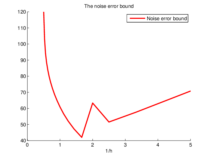
Now, we study the influence of on the noise error contribution. The variations of is shown in Figure 3(b). Moreover, we can verify that the number of the negative eigenvalues and are equal. We can see their variation with respect to in Figure 3(d). Consequently, according to Figure 3(b) and Figure 3(d) we can observe that when is equal to the noise error contribution is increasing with respect to . However, when the value of increases, the noise error contribution is decreasing with respect to . Consequently, a small value of can produce a large noise error contribution.
We are going to use Proposition 5 to deduce the variation of the noise error contribution with respect to . Since the noise is assumed to be a zero-mean white Gaussian sequence, by using the well known three-sigma rule we obtain that
| (46) |
The variation of the noise error bounds given in Proposition 5 is shown in Figure 3(c). Although this error bound is not sharp, its variation is similar to the one of the noise error contribution shown in Figure 3(b), where there are local minimums at and , and a local maximum at .
Finally, by combined with the variation of shown in Figure 3(a), we can choose or in our estimation so as to minimize the total estimation error.



VI conclusion
In this paper, the SCSA method recently introduced for signal analysis is studied in discrete noisy case. Some mathematical properties of the negative eigenvalues of a Schrodinger operator are given in discrete noise-free case and discrete noisy case respectively. An a-posteriori error bound of the noise error contribution is given which is based on the expected value and the variance of a corrupting noise. By taking a numerical example, we show the influence of the semi-classical parameter on different sources of errors in the SCSA method. Moreover, it is shown that the SCSA method is accurate and robust against corrupting noises. Hence, it can be considered as a filter without involved delays. Finally, we study how to choose an appropriate semi-classical parameter without knowing the original signal. The comparison to other signal analysis methods like Fourier transform or the wavelets will be done in a future work. Moreover, the SCSA method will be extended for time derivatives filtering, which is still an open problem, such that this method can be useful in more applications in signal processing and automatic control.
References
- [1] T. M. Laleg-Kirati, E. Crépeau and M. Sorine, Semi-classical signal analysis, to appear in Mathematics of control signals and systems (MCSS) journal, 2012
- [2] M. Dimassi and J. Sjöstrand, Spectral asymptotics in the semi-classical limit, Cambridge U Press, 1999.
- [3] L. D. Faddeev, Properties of the S-matrix of the one-dimensional Schrödinger equation, Trudy Mat. Inst. Steklov, 73, pp. 314-336, 1964.
- [4] T. M. Laleg-Kirati, C. Médigue, F. Cottin and M. Sorine, Arterial blood pressure analysis based on scattering transform II, in Proc. EMBC, Lyon, France, August 2007.
- [5] T. M. Laleg-Kirati, C. Médigue, Y. Papelier, F. Cottin and A. Van de Louw, Validation of a semi-classical signal analysis method for stroke volume variation assessment: A comparison with the PiCCO technique, Annals of biomedical engineering, vol. 38, no. 12, pp. 3618-3629, 2010.
- [6] F. Eleiwi, T. M. Laleg-Kirati, S. Khelladi and F. Baki, A Semi-Classical Signal Analysis Method for the Analysis of Turbomachinery Flow Unsteadiness, World Academy of Science, Engineering and Technology, vol. 59, pp. 215-218, 2011.
- [7] M. Fliess, Analyse non standard du bruit, C.R. Acad. Sci. Paris Ser. I, 342, pp. 797-802, 2006.
- [8] D. Y. Liu, O. Gibaru, W. Perruquetti, M. Fliess and M. Mboup, An error analysis in the algebraic estimation of a noisy sinusoidal signal. In: 16th Mediterranean conference on Control and automation (MED’08), Ajaccio, France, 2008.
- [9] D. Y. Liu, O. Gibaru and W. Perruquetti, Error analysis for a class of numerical differentiator: application to state observation, 48th IEEE Conference on Decision and Control, Shanghai, China, 2009.
- [10] D. Y. Liu, O. Gibaru and W. Perruquetti, Error analysis of Jacobi derivative estimators for noisy signals. Numerical Algorithms, 58, 1, pp. 53-83, 2011.
- [11] D. Y. Liu, O. Gibaru and W. Perruquetti, Convergence Rate of the Causal Jacobi Derivative Estimator. Curves and Surfaces 2011, LNCS 6920 proceedings, pp. 45-55, 2011.
- [12] D. J. Kaup and A. C. Newell, Solitons as particles, oscillators, and in slowly changing media: a singular perturbation theory, Proc. R. Soc. Lond. A. 361, pp. 413-446, 1978.
- [13] J. P. Boyd, Chebyshev and Fourier Spectral Methods, Dover Publication, Inc., 2nd edition, 2000.
- [14] L. N. Trefethen, Spectral Methods in Matlab, SIAM, 2000.
- [15] G. Stewart and J. G.Sun, Matrix Perturbation Theory, Academic Press, New York, 1990.
- [16] G. Olafsson and S. Zheng. Function spaces associated with Schrodinger operators: the Poschl-Teller potential. Journal of Fourier Analysis and Applications, 12(6), pp. 653-674, 2006.
- [17] G. Bianchi and R. Sorrentino, Electronic Filter Simulation & Design. New York: Mc Graw-Hill, 2007.