Supplementary Material for Discovering associations that replicate from a primary study of high dimension to a follow-up study
Discovering findings that replicate from a primary study of high dimension to a follow-up study
Marina Bogomolov and Ruth Heller11
1
Address for correspondence: Department of
Statistics and Operations Research, Tel-Aviv university, Tel-Aviv,
Israel. E-mail: ruheller@post.tau.ac.il. This work was supported by grant no. 2012896 from the
Israel Science
Foundation (ISF). The authors thank Yoav Benjamini, Daniel Yekutieli, and the referees for helpful comments.
Technion and Tel-Aviv University
Abstract. We consider the problem of identifying whether findings replicate from one study of high dimension to another, when the primary study guides the selection of hypotheses to be examined in the follow-up study as well as when there is no division of roles into the primary and the follow-up study. We show that existing meta-analysis methods are not appropriate for this problem, and suggest novel methods instead. We prove that our multiple testing procedures control for appropriate error-rates. The suggested FWER controlling procedure is valid for arbitrary dependence among the test statistics within each study. A more powerful procedure is suggested for FDR control. We prove that this procedure controls the FDR if the test statistics are independent within the primary study, and independent or have dependence of type PRDS in the follow-up study. For arbitrary dependence within the primary study, and either arbitrary dependence or dependence of type PRDS in the follow-up study, simple conservative modifications of the procedure control the FDR. We demonstrate the usefulness of these procedures via simulations and real data examples.
Keywords: False discovery rate; genome-wide association studies ; meta-analysis; multiple comparisons; replicability analysis
1 Introduction
In genomics research, it is customary that a primary study is followed by an independent study. Reporting results from the primary study, and then reporting the evidence from the follow-up study that supports these results, gives a sense of the replicability of the results. For example, findings are informally regarded as replicated if the -value for testing a null hypothesis is small in the primary study, and then for the same hypothesis the -value is fairly small in the follow-up study.
Many approaches are available for analyzing two or more studies, where the follow-up studies simply serve to add power. See Hedges and Olkin, (1985), Benjamini and Yekutieli, (2005), Skol et al., (2006), and Zeggini et al., (2007), among others. In this work, we focus on analyzing two studies, where the follow-up study serves to confirm the findings that were identified in the primary study. A formal statistical approach is proposed for evaluating whether results from a primary study were indeed replicated in a follow-up study.
In observational studies, an association may fail to replicate because the discovered association was not the actual effect of a treatment but rather that of bias (Rosenbaum,, 2001). However, if the finding is replicated in a different cohort, using different diagnostic or laboratory methods, then the association between effect and outcome may be more convincingly causal. Rosenbaum, (2001) gives the example of radiation and leukemia. Suppose higher rates of leukemia are discovered in a primary study among radiologists, and in a follow-up study among survivors at Hiroshima and Nagasaki. Radiation is more convincingly causal if the association discovered was replicated in the follow-up study, since if radiation was not a cause of leukemia, then higher rates of leukemia among radiologists would not lead us to expect higher rates of leukemia among survivors at Hiroshima and Nagasaki. Another example comes from the field of genomic research. Genome-wide association studies (GWAS) are observational studies, and therefore there is always a danger that bias may explain away the discoveries. Kraft et al., (2009) note that for common variants, the anticipated effects are modest and very similar in magnitude to the subtle biases that may affect genetic association studies - most notably population stratification bias. For this reason, they argue that it is important to see the association in other studies conducted using a similar, but not identical, study base.
It is common practice that interesting findings in a primary GWA study are investigated in another study, and the interesting results of both studies are reported (Lander and Kruglyak,, 1995). For example, to discover association between single-nucleotide polymorphisms (SNPs) and hippocampal volume, Bis et al., (2012) tested SNPs in a primary study, and only a handful of SNPs in promising loci in a follow-up study. Bis et al., (2012) forwarded a SNP for replication if the SNP -value in the primary study was below , corresponding to one expected false positive if all SNPs are not associated with hippocampal volume. They viewed the SNP as containing evidence of replication if its -value in the follow-up study was below 0.01, which is the Bonferroni threshold when 5 hypotheses are simultaneously tested at the 0.05 family-wise error rate (FWER). Their approach selects hypotheses for follow-up based on suggestive evidence (Lander and Kruglyak,, 1995), and corrects for multiplicity only in the follow-up study when discussing evidence of replicability. Another naive approach is the following: apply a multiple testing procedure within each study separately, and declare as replicated the common findings. This approach will lead to declaring SNPs that were found to be associated with the disease in the primary study as well as in the follow-up study as the discoveries of interest. If there was no danger that a multiple testing procedure produces false positives, then this naive approach would have been appropriate. However, multiple testing procedures have a non-zero probability of producing false positives, unless they have no power. Therefore, an approach that provides control over false positives in each study separately, does not guarantee control over false positives for evaluating whether the results were replicated. Figure 3, left panel, shows that the FDR level can be as high as one when naively declaring results as replicated if they were discovered by applying an FDR controlling procedure at the nominal 0.05 level separately in each study. Moreover, reducing the nominal 0.05 level does not resolve the problem, see Remark 3.1.
The paper is organized as follows. Section 2 gives the notation and review. Section 3 suggests novel multiple testing procedures for replicability analysis, when the primary study guides the selection of hypotheses to be examined in a follow-up study. Section 4 considers the setting where there is no division of roles into a primary and a follow-up study. In Section 5, we revisit the example of Bis et al., (2012). We also analyze an additional GWAS study, and show additional examples from the GWAS simulator HAPGEN2 (Su et al.,, 2011). Section 6 describes a simulation study, and Section 7 gives some final remarks.
2 Notation, Goal, and Review
Consider a family of elementary null hypotheses . These elementary null hypotheses, or a subset thereof, are tested in each of two independent studies. Let be the indicator of whether is false in study . The pair of indicators identifies four possible settings for each ,
The set of indices of the elementary null hypotheses may be divided into four (unknown) subsets , where each index is in exactly one of the four subsets, defined as follows:
Definition 2.1.
The no replicability null hypothesis for elementary hypothesis is
By definition, is false if and only if the elementary null hypothesis is false in both studies considered. In the family of composite null hypotheses , the sets of indices of true and false null hypotheses are and respectively. Our goal is to discover as many indices from as possible, i.e. true positives, while controlling for the number of discoveries from , i.e. false positives.
Let be the -value for the th SNP in study , for . Since the studies are independent, the -values are independent across studies. However, the -values within each study may be dependent. Inequality for vectors and is understood componentwise.
Remark 2.1.
In a typical meta-analysis (Hedges and Olkin,, 1985), the goal is to discover as many indices from as possible, while controlling for the number of discoveries from . Had we known, and had it been true, that and , then the typical methods for meta-analysis could serve to discover replicable findings. However, it is not known in practice whether and are empty sets, and they need not be empty when the follow-up study is different, in at least one aspect of design, from the primary study. Therefore, typical meta-analysis methods are not appropriate when the aim is to discover hypotheses with indices in , treating all discoveries from and , in addition to , as false discoveries.
2.1 The partial conjunction approach
In Benjamini et al., (2009) the partial conjunction approach (Benjamini and Heller,, 2008) has been suggested for replicability analysis when studies are available that examine the same problem. When exactly two studies are available, the procedure in Benjamini et al., (2009) amounts to applying the Benjamini-Hochberg false discovery rate (FDR) controlling procedure (Benjamini and Hochberg,, 1995), henceforth referred to as the BH procedure, on the maximum of the two study -values. However, this procedure may be too conservative, making it practically very difficult to discover false no replicability null hypotheses.
As an example, suppose there is an original GWA study that examines the association of SNPs with a phenotype. Now suppose 200 promising SNPs were selected to be examined in a follow-up study. If a SNP has a -value of in the first study, and of in the second study, then the maximum -value is . The BH procedure will, most probably, not reject the no replicability null hypothesis for a SNP with maximum -value of , since this maximum -value is not strong enough evidence when faced with hypotheses, out of which most of the hypotheses are true no replicability null hypotheses. The alternative procedures we suggest in Sections 3 and 4 will view the evidence from this SNP as strong enough for it to be considered a replicated finding.
3 Replicability analysis with a primary and a follow-up study
For the family of no replicability null hypotheses , we consider two relevant error measures: the probability that at least one no replicability null hypothesis is falsely rejected, i.e. the FWER, and the expected fraction of false rejections out of all rejections of no replicability null hypotheses, that is the FDR.
Procedure 3.1.
The two stage FWER controlling procedure for testing the family of no replicability null hypotheses with parameters , where :
- 1.
Let be the set of indices of elementary hypotheses that are selected for testing in a follow-up study based on the data from the primary study.
- 2.
Apply a FWER controlling procedure at level , using the data from the primary study only, on the family of null hypotheses , and let be the set of indices of rejected hypotheses. Apply a FWER controlling procedure at level , using the data from the follow-up study only, on the family of selected null hypotheses , and let be the set of indices of rejected hypotheses. Then the set of indices of rejected no replicability null hypotheses is .
Theorem 3.1.
For two independent studies, Procedure 3.1 controls the FWER at level for the family of no replicability null hypotheses .
Proof.
Let and be the number of true elementary null hypotheses rejected, respectively, in the primary study and in the follow-up study. Then
where the last inequality follows from the fact that is independent of the data from the primary study, and that in both studies a FWER controlling procedure is applied.
Using Bonferroni in Procedure 3.1 amounts to rejecting if , for . Alternatively, the results can be reported in terms of Bonferroni-replicability adjusted -values , where . Procedure 3.1 using Bonferroni is equivalent to rejecting all hypotheses with Bonferroni-replicability adjusted -values at most .
The selection rule affects the power of Procedure 3.1. A natural choice for a selection rule is the set of rejected hypotheses by the FWER controlling procedure at level on the primary study -values, since the set of indices of rejected no replicability null hypotheses is a subset of this set. A rule that selects by the FWER controlling procedure at level is not as good, since any additional hypotheses selected will not be rejected but will result in a more severe multiple testing problem for the follow-up study. The choice of also affects the power of Procedure 3.1. We observed in simulations (Supplementary Material) that although the optimal varies with effect size, the power function is quite flat as long as is not too close to zero or one.
In many modern applications, controlling the FWER is unnecessary and results in overly conservative inferences. In genomics research, it is often enough to guarantee FDR control, see Storey and Tibshirani, (2003) and Reiner et al., (2003), among others.
Procedure 3.2.
The two stage FDR controlling procedure for testing a family of no replicability null hypotheses with parameters , where :
- 1.
Let be the set of indices of elementary hypotheses that are selected for testing in a follow-up study based on the data from the primary study. Let be the cardinality of this set.
- 2.
Let
Then the set of indices of rejected no replicability null hypotheses is
The results of Procedure 3.2 can be reported in terms of FDR-replicability adjusted -values. Let ,
| (3.1) |
and let be the sorted -values. Then the th largest FDR-replicability adjusted -value is
| (3.2) |
Procedure 3.2 with parameters is equivalent to rejecting all no replicability null hypotheses with FDR-replicability adjusted -values at most .
Definition 3.1.
A valid selection rule for step 1 of Procedure 3.2 satisfies the following condition: for any , fixing all the -values except for and changing so that is still selected, will not change the set .
It is easy to see that this condition is satisfied if contains the smallest fixed number of -values, all hypotheses with -value below a given threshold, or if contains the rejected indices from a BH procedure on the -values from the primary study. Adaptive FDR procedures on the -values from the primary study, e.g. Benjamini and Hochberg, (2000), Storey et al., (2004), Benjamini et al., (2006), and Blanchard and Roquain, (2009), are non-valid selection rules.
Theorem 3.2.
See Appendix A for the proof.
The selection rule and the choice of affect the power of Procedure 3.2. A natural choice for a selection rule is the set of rejected hypotheses by the BH procedure at level on the primary study -values, since the set of indices of rejected no replicability null hypotheses is a subset of this set. A rule that selects by the BH procedure at level is not as good as the rule at level , since any additional hypotheses selected will not be rejected, but will result in more severe thresholds on the follow-up study -values. In Figure 4 we showed in a simulated example that the BH procedure at level was very close to selecting the optimal number of hypotheses for follow-up. We recommend using it when there are no additional constraints that require choosing only a small number of hypotheses for follow-up. The optimal choice of depends on , and the non-null distribution of the -values, and therefore guidelines for choosing are application specific. In simulated GWAS in Section 5 the choice of had little effect on the average number of discoveries.
Theorem 3.2 assumes independence of the -values within each study as well as across the studies. However, the assumption of independence among the -values within each study may not be realistic in many applications. Particularly, in GWAS there is dependency across the SNPs, therefore the -values within each study may be dependent. Benjamini and Yekutieli, (2001) proved that the BH procedure controls the FDR when the -values have a special dependency called PRDS.
Definition 3.2.
(Benjamini and Yekutieli,, 2001) The set of -values has property PRDS if for any increasing set , and for each true null hypothesis , is nondecreasing in .
If the -values are independent in the primary study, yet have property PRDS in the follow-up study, Theorem S3.1 in the Supplementary Material shows that the result in Theorem 3.2 holds. For arbitrary dependence among the -values in the primary study, a modification of the cut-off level of Procedure 3.2 will guarantee that the FDR is controlled at the nominal level. The most severe modification, that will guarantee FDR control for any valid selection rule, is to apply Procedure 3.2 with the modification in item 1 of Theorem 3.3 below. However, in item 2 of Theorem 3.3 we show that the modification factor may be smaller than if the selected hypotheses for follow-up are a subset of the hypotheses with primary study -values below a fixed cut-off . For example, in GWAS it is common to select hypotheses with primary study -values below , where is the number of hypotheses in the primary study (Lander and Kruglyak,, 1995). If , then the modification in item 1 of Theorem 3.3 cannot be improved. However, if , then the modification in item 2 of Theorem 3.3 is less conservative than the modification in item 1. For typical values of (e.g. ) and large , the threshold will often be below , and therefore item 2 may be useful in applications. Note, moreover, that if , then item 2 of Theorem 3.3 states that no modification is required, so for a valid selection rule which selects a subset of the set of hypotheses with primary study -values below , where , Procedure 3.2 is valid for any form of dependency among the -values in the primary study.
Theorem 3.3.
Assume that the follow-up study -values have property PRDS, and are independent of the -values in the primary study. Then Procedure 3.2 controls the FDR at level for the family of no replicability null hypotheses if the selection rule used in step 1 of Procedure 3.2 is a valid selection rule, and the expressions in step 2 of Procedure 3.2 are modified as follows:
- 1.
In the terms and only, is replaced by .
- 2.
In the terms and only, is replaced by , where
if only hypotheses with primary study -values at most a fixed threshold are considered for follow-up, i.e. , where .
See Supplementary Material for the proof, as well as for additional results under dependency. Specifically, Theorem S3.2 in the Supplementary Material shows that in the more general setting of arbitrary dependence among the follow-up study -values, it is also necessary to replace with in the terms and in expression 2 of Procedure 3.2. These results are similar to the result in Benjamini and Yekutieli, (2001) for the BH procedure in their Theorem 1.3.
Remark 3.1.
Benjamini and Yekutieli, (2005) proved in their Proposition 3 that the procedure that applies the BH procedure at level on the primary study -values, and the BH procedure at level on the follow-up study -values, controls the FDR at level on the family of global null hypotheses, , where . However, on the family of no replicability null hypotheses, , the FDR of this procedure may be higher than the nominal level . The key difference between Procedure 3.2 and such a two stage procedure, is the requirement that the two -values from a selected hypothesis have to simultaneously be smaller than two thresholds. In an extreme scenario where all hypotheses are from or , and the -values from false null hypotheses are zero, the two stage procedure may have an FDR of one, as follows. The BH procedure on the primary study -values will reject all hypotheses from but also few from (when and are large enough), and the hypotheses from will be rejected by the BH procedure on the follow-up study -values, resulting in an FDR of one. However, Procedure 3.2 will have an FDR level below . To see this, note that in order to reject a no replicability null hypothesis by Procedure 3.2, the -value of the Simes test (Simes,, 1986) for the intersection of the elementary hypotheses indexed by , using the data from the primary study, has to be below , or the Simes test -value for the intersection of elementary hypotheses indexed by , using the data from the follow-up study, has to be below . Therefore, the probability of rejecting at least one no replicability null hypothesis, which coincides with the FDR since all no replicability null hypotheses are true, is at most . See Figure 3, right panel, for a more realistic simulated example.
4 Replicability analysis with no division into primary and follow-up studies
Consider now a situation where both studies are available before the analysis. If some of the elementary hypotheses are examined in only one of the studies, then these hypotheses are not considered for replicability analysis. In this setting, there is no primary study and follow-up study. We propose the following generalization of Procedure 3.2, that can be tuned to treat the two studies symmetrically. Without loss of generality, we label the studies as study one and study two.
Procedure 4.1.
The generalized two stage procedure for testing a family of no replicability null hypotheses with parameters , where and :
- 1.
Apply Procedure 3.2 with parameters with study one as the primary study and study two as the follow-up study. Denote the set of indices of rejected no replicability null hypotheses by .
- 2.
Reverse the roles of study one and study two. Apply Procedure 3.2 with parameters . Denote the set of indices of rejected no replicability null hypotheses by .
- 3.
The set of indices of rejected no replicability null hypotheses is .
Theorem 4.1.
See Appendix C for the proof.
Choosing results in Procedure 3.2, where study one has the role of the primary study and study two has the role of the follow-up study. Similarly, choosing results in Procedure 3.2 with the roles of study one and study two reversed. The choice reflects the similarity of Procedure 4.1 to Procedure 3.2 in the following way: when is close to one (zero), Procedure 4.1 gives similar results to Procedure 3.2 with study one (two) as the primary study. The choice results in a variant of Procedure 3.2 that is symmetric with respect to both studies.
5 GWAS examples
In this section we demonstrate the suggested methods on two real data examples and on a GWAS simulation. A replicability analysis with FWER control is carried out for the first example, that has only five hypotheses in the follow-up study. A replicability analysis with FDR control is carried out for the second example, that has 126 hypotheses in the follow-up study. Finally, in order to examine the robustness of procedure 3.2 for GWAS type dependency, examples were simulated that retained the dependencies in the data that occur in GWAS.
Example 1.
We reproduce in Table 1, columns 1-4, a subset of the columns of Table 1 of results of Bis et al., (2012). We added in columns 5-7 the Bonferroni-replicability adjusted -values for . Procedure 3.1 with parameters or identified the SNP near MSRB3 as having replicated association with the phenotype. The choice of should be made prior to analysis, and the choice may be preferred over when it is believed that the power to detect an association in the primary study using a threshold of order is smaller than the power to detect an association in the follow-up study using a threshold of order .
| Locus | Gene | Primary | Follow-up | Bonferroni-replicability adjusted -values | ||
|---|---|---|---|---|---|---|
| study | study | |||||
| 2q24 | DPP4 | 0.7 | 1.0000 | 1.0000 | 1.0000 | |
| 9q33 | ASTN2 | 0.2 | 1.0000 | 0.5000 | 0.3125 | |
| 12q14 | MSRB3 | 0.002 | 0.06875 | 0.0275 | 0.0172 | |
| WIF1 | 0.0007 | 0.2750 | 0.1100 | 0.0688 | ||
| 12q24 | HRK | 0.6000 | 0.2400 | 0.1500 | ||
Example 2.
To discover associations between SNPs and Crohn’s disease (CD), Barrett et al., (2008) examined 635,547 SNPs on 3230 cases and 4829 controls of European descent, collected in three separate studies: NIDDK4, WTCCC5, and a Belgian-French study. The primary study -values in this example are the meta-analysis -values from the combined data from the three studies. Only hypotheses with primary study -values below were considered for follow-up. Although 526 SNPs met the selection criterion, only a subset of 126 SNPs were followed up. These 126 -values were the smallest two -values in 63 distinct regions, so the selection rule is a valid selection rule. Procedure 3.2 with identified 36 SNPs. In Appendix D, Table 5 shows the -values from the primary and follow-up studies, as well as the FDR-replicability adjusted -values for the choice , for these 36 replicability discoveries. Since the -values are not independent within each study, a more conservative analysis approach is to modify the cut-offs as suggested by Theorem 3.3. Assuming PRDS type dependency in the follow-up study, item 1 of Theorem 3.3 suggests using for the primary study cut-offs, while the follow-up study cut-offs remain unchanged. The modified procedure identified 21 SNPs. Column 7 of Table 5 shows the FDR-replicability adjusted -values for the choice , where the adjustment is made as described in expressions (3.1) and (3.2), with replaced by . Since the SNPs considered for follow-up were only SNPs with primary study -values below , one could use a less conservative procedure suggested in item 2 of Theorem 3.3, with , where is the solution to . This procedure resulted in 23 replicability discoveries. The latter procedure is the recommended procedure, if the investigator is not willing to assume that Procedure 3.2 is robust to deviations from independence within the primary study. However, simulations in the next example suggest that for the type of dependencies that occur in GWAS, Procedure 3.2 may actually be conservative. We come back to the issue of robustness of Procedure 3.2 in the Discussion Section 7.
GWAS simulation example.
We simulated two GWAS from the simulator HAPGEN2 (Su et al.,, 2011). The two studies were generated from two samples of the HapMap project (The International HapMap Consortium,, 2003), a sample of 165 Utah residents with Northern and Western European ancestry (CEU), and a sample of 109 Chinese in Metropolitan Denver, Colorado (CHD). In the CEU and CHD populations, respectively, 34 and 38 SNPs were set as disease SNPs with an increased multiplicative relative risk of 1.2, and 18 of the disease SNPs were common to both populations. Each study contained 4500 cases and 4500 referents. The linkage disequilibrium (LD) across SNPs, as measured for the samples in the HapMap project, was retained. Due to LD, the number of SNPs associated with the phenotype in each study was larger than the number of disease SNPs. In order to identify the SNPs in each study that are truly associated with the phenotype, the simulation of 4500 cases and 4500 controls from the population was repeated 11 times, and 11 -values were produced per SNP. SNPs with Fisher’s combined -value (Loughin,, 2004) below the Bonferroni threshold were considered to be truly associated with the disease. Our ground truth included 1355 and 1010 SNPs associated with the disease in the CEU and in the CHD population, respectively, out of which 274 SNPs were associated with the disease in both populations.
As a standard preprocessing step, we removed SNPs with minor allele frequency below 0.05, and thus the number of SNPs in the analysis was reduced from 1,387,466 to 887,362, on average, for the 11 pairs of studies. Our selection rule for Procedure 4.1 with parameters was the BH procedure at level when the primary study was the CEU study, and at level when the primary study was the CHD study, since the potential set of SNPs to be discovered as having replicated associations is at most the set of SNPs that are discovered by the BH procedure (as discussed in Section 3). Table 2 presents the average number of replicated findings, as well as the average false discovery proportion (FDP) for the methods compared. The standard error (SE) is presented in parentheses. From rows 1 and 2 we see that if there is no division into primary and follow-up studies, then the symmetric Procedure 4.1 discovers more SNPs with replicated associations than the BH procedure on maximum -values, while maintaining a low FDP. From rows 3-5, and 6-8, we see that the choice of which study was the primary study had a large effect on the average number of discoveries, and the choice of mattered little.
| Procedure | # Replicated findings | FDP | |
|---|---|---|---|
| associated SNPs (SE) | disease SNPs (SE) | (SE) | |
| BH on maximum -values | 29.182 (3.205) | 7.364 (0.432) | 0.000 (0.000) |
| 4.1 with | 77.727 (6.378) | 11.455 (0.366) | 0.011 (0.005) |
| 4.1 with | 74.091 (6.748) | 10.364 (0.310) | 0.012 (0.006) |
| 4.1 with | 76.091 (6.221) | 10.727 (0.359) | 0.012 (0.005) |
| 4.1 with | 69.545 (5.745) | 10.818 (0.352) | 0.009 (0.005) |
| 4.1 with | 35.545 (4.575) | 7.364 (0.607) | 0.008 (0.008) |
| 4.1 with | 41.455 (5.294) | 8.273 (0.469) | 0.007 (0.007) |
| 4.1 with | 42.273 (4.158) | 8.545 (0.312) | 0.000 (0.000) |
From the last column in Table 2 we see that the average FDP was far below 0.05, suggesting that the procedures are conservative. This conservatism can be alleviated if the following oracle information were known: the fraction of SNPs with no association with the phenotype in both studies, , and with association with the phenotype only in the follow-up study, . Then it was possible to perform Procedure 4.1 at level , where is the solution to for , and the solution to for , with the same guarantee of FDR control at level , as follows from Appendix B. Specifically, in our simulation , on average, after preprocessing. For FDR control at level , on average for and for . Table 3 shows the average FDP and average number of rejections for Procedure 4.1 with and without the oracle. Although the average FDP is higher with the oracle, it is still below the nominal 0.05 level for two main reasons. First, our simulation preserves the LD pattern of the SNPs, and thus the -values within each study are not independent. Second, the upper bound of is not a tight upper bound for the actual FDR level. A tighter oracle upper bound requires knowing the expectation of , and this bound is tight if the non-null effect sizes in are extremely large.
| FDP | # Replicated findings | |||
|---|---|---|---|---|
| Oracle | Oracle | |||
| 0.023 | 0.011 | 90 | 78 | |
| 0.023 | 0.012 | 85 | 76 | |
| 0.029 | 0.007 | 50 | 41 | |
For the two studies from the CEU and CHD populations, a meta-analysis was performed by first combining the SNP -values using Fisher’s combining method, and then applying the BH procedure at level 0.05 on the combined -values. The average number of SNPs associated with the disease in at least one study was 393, while less than 80 SNPs were discovered to have replicated associations (Table 2). The two main reasons for discovering more SNPs in a typical meta analysis are as follows. First, the simulation setting contained five times more associated SNPs than SNPs with replicated associations. Second, for a SNP with a replicated association, the power to detect that the association is replicated is lower than the power to detect that there is an association in at least one study. The discovered SNPs with replicated associations were a subset of the discovered associated SNPs, but their meta-analysis -values were not ranked smallest among all meta-analysis -values (not shown). Importantly, the discoveries from the meta-analysis could not serve as evidence towards replicability, since while the average fraction of SNPs with no association in both studies among the meta-analysis discoveries was 0.06, the average fraction of SNPs with no replicated association among the meta-analysis discoveries was 0.78.
6 A simulation study
The goal of the simulations was threefold. First, to investigate the effect of the choice of and on the power of Procedures 3.2 and 4.1. Second, to compare these procedures to the alternative of applying BH on the maximum -values, i.e. the partial conjunction approach when exactly two studies are analyzed. Third, to investigate the effect of the selection rule on the power of the procedures.
The procedures compared were (1) the BH procedure at level 0.05 on maximum -values; (2) Procedure 4.1 with , , and ; and (3) the naive (BH-, BH-) procedure, , , which applies the BH procedure at level 0.05 on the -values of study , and separately on the -values of study for the hypotheses that were rejected in study , and declares hypotheses rejected in both studies as false no replicability null hypotheses; (4) the oracle Procedure 3.2 with parameters , where was the solution to . This oracle procedure controls the FDR at level , see Appendix B for a proof.
The -values were generated independently as follows. For , , and , where and . We let , where , and . We set , and for as follows: , ; , , ; ; , . The standard deviations and were either fixed values , , or reflected the fraction of sample size allocated to the first study: , , , , .
The simulation results were based on 1000 repetitions. The FDR was estimated by averaging the FDP. The average power was estimated by the average number of rejected false no replicability null hypotheses, divided by .
6.1 Simulation results
As expected from our theoretical results, in all the settings considered the estimated FDR was below 0.05 for all procedures but the naive (BH-, BH-) procedure. The SE of the estimated FDR and power were of the order of for all procedures under all configurations considered.
Figure 1 compares the power of the BH procedure on maximum -values, (1) above, and Procedure 4.1 with , , (2) above, in a configuration with parameters . The oracle Procedure 3.2, where the primary study is study one with , is also examined. For each procedure the estimated power and FDR is shown as a function of the common expectation under the alternative, . Procedure 4.1 with is more powerful than with or , while the choice is the worst in terms of power of Procedure 4.1. Moreover, Procedure 4.1 with is more powerful than the BH procedure on maximum -values. These findings were consistent across all configurations of examined, when and . Since the oracle Procedure 3.2 and the BH procedure on maximum -values do not depend on , their power curves are the same in figures (a), (b), and (c). We see that Procedure 4.1 with is a close second to the oracle when is 0.01 but is farther from the oracle as increases. Similarly, the power of Procedure 4.1 with decreases as increases. However, Procedure 4.1 with has largest power for , and the least power for . These results are reasonable since the -values of study one tend to be much smaller than the -values of study two when the no replicability null hypotheses are false. In Table 4 we see that if the -value distribution of false no replicability null hypotheses is the same across studies, then the optimal choice of is . For example, when (row 2), the power is 0.65 with , 0.77 with , and the maximum power is 0.81 with .
| 0.1 | 0.2 | 0.3 | 0.4 | 0.5 | 0.6 | 0.7 | 0.8 | 0.9 | |
|---|---|---|---|---|---|---|---|---|---|
| 1.5 | 0.143 | 0.195 | 0.224 | 0.245 | 0.257 | 0.258 | 0.248 | 0.226 | 0.181 |
| 2.0 | 0.646 | 0.718 | 0.755 | 0.778 | 0.794 | 0.803 | 0.805 | 0.800 | 0.769 |
| 2.5 | 0.934 | 0.955 | 0.965 | 0.971 | 0.975 | 0.977 | 0.978 | 0.978 | 0.974 |
Figure 2 compares the procedures (1) and (2) above for the same configuration of , but for fixed and varying sample size of the two studies. The varying power is described by the fraction of sample allocated to the first study. For the symmetric procedures, we see that for the power is the lowest, and it increases to reach its maximum for equal allocation . Procedure 4.1 with dominates the BH procedure on the maximum two study -values. For Procedure 4.1 with , the maximum is reached for . It is the most powerful of the three procedures examined for .
In Figure 3 we consider the FDR level of Procedure 4.1 with , as well as of the naive procedure in the null setting, where all no replicability null hypotheses are true (i.e. ). The estimated FDR of (BH-, BH-) procedure exceeds 0.05 in the settings where and . In these settings the estimated FDR of both (BH-, BH-) and (BH-, BH-) procedures are increasing functions of , reaching one in the setting where (left), and 0.4 in the setting where (right). Clearly, procedure (BH-, BH-) is not valid since it may be far too liberal in terms of FDR level.
Finally, we examined how the selection rule affects the power. In Figure 4 we show the power as a function of for Procedure 4.1 with parameters , for the following selection rules: BH at level ; the rule that selects the hypotheses with smallest primary study -values, where . The remaining parameters were: . For different values of the optimal is different, and using the BH procedure for selection is optimal for the entire range of .


7 Discussion
In many research areas first a primary study is analyzed, then a follow-up study is analyzed with the goal to corroborate the findings, or at least a subset of the findings, of the primary study. We suggested novel testing procedures for corroborating the evidence from a primary study in a follow-up study. We demonstrated their usefulness on a GWAS application. In the setting where there is no division of roles to a primary and a follow-up study, the simulations suggested that our novel Procedure 4.1 with is more powerful than the BH procedure on maximum -values.
We proved that Procedures 3.2 and 4.1 control the FDR when the -values are independent within each study and the selection rule is valid. However, the assumption of independence may not be realistic. Extensive simulations demonstrated that the BH procedure controls the FDR for many types of dependence encountered in practice (Yekutieli,, 2008). We conjecture that this robustness property carries over to Procedures 3.2 and 4.1, since Procedure 3.2 can be viewed as two-dimensional variant of the BH procedure. For simulated GWAS examples the average false discovery proportion was below the nominal FDR level, suggesting that the procedures are indeed valid for the type of dependency that occurs in GWAS. More conservative variants of Procedure 3.2 were given in Theorem 3.3 and in Section 3 of the Supplementary Material, that guarantee that the FDR is controlled for arbitrary dependence among the primary study -values, and dependence of type PRDS or arbitrary dependence among the follow-up study -values. We demonstrated the usefulness of the variants suggested in Theorem 3.3 in Example 2 of Section 5. Out of the 36 replicability discoveries with Procedure 3.2, 23 discoveries passed the more stringent requirement that came with the added guarantee that the FDR is controlled for arbitrary dependence among the 635,547 -values in the primary study.
Replicability analysis, as suggested in this paper, requires that the investigators make several key design choices in addition to the error level : the selection rule, , and if two studies are available without division into primary and follow-up. The power of the procedure for replicability analysis varies with these choices. From our investigations, it appears reasonable in Procedure 3.2 to select hypotheses by BH at level , and to set in Procedure 4.1 if the -value distributions for false null hypotheses may be assumed to be similar in both studies. We gave some guidelines for choosing in specific settings, and more general guidelines are a topic for future research.
In replicability analysis, the primary study guides the design of the follow-up study by supplying the subset of hypotheses to be followed-up. Since the primary study also yields information on effect sizes, if it is assumed that the effect sizes are the same across studies, then this information may be used in order to determine the sample size needed to obtain good power in the follow-up study. However, this assumption may be unrealistic in applications such as GWAS, where the LD pattern varies across populations.
Finally, we saw that although Procedure 4.1 with parameters is far less conservative than the BH procedure at level on maximum -values, it is still conservative. We proved that Procedure 4.1 with less conservative parameters and , still controls the FDR at level on the family of no replicability null hypotheses, if and were known. In future research we will consider estimates of these unknown parameters.
References
- Barrett et al., (2008) Barrett et al. (2008). Genome-wide association defines more than 30 distinct susceptibility loci for Crohn’s disease. Nature Genetics, 40: 955–962.
- Benjamini and Heller, (2008) Benjamini, Y. and Heller, R. (2008). Screening for partial conjunction hypotheses. Biometrics, 64:1215–1222.
- Benjamini et al., (2009) Benjamini, Y., Heller, R., and Yekutieli, D. (2009). Selective inference in complex research. Philosophical Transactions of the Royal Society A (accepted), 267:1–17.
- Benjamini and Hochberg, (1995) Benjamini, Y. and Hochberg, Y. (1995). Controlling the false discovery rate - a practical and powerful approach to multiple testing. J. Roy. Stat. Soc. B Met., 57 (1):289–300.
- Benjamini and Hochberg, (2000) Benjamini, Y. and Hochberg, Y. (2000). On the adaptive control of the false discovery fate in multiple testing with independent statistics. Journal of educational and behavioral statistics, 25(1):60–83.
- Benjamini et al., (2006) Benjamini, Y., Krieger, M., and Yekutieli, D. (2006). Adaptive linear step-up false discovery rate controlling procedures. Biometrika, 93 (3):491–507.
- Benjamini and Yekutieli, (2001) Benjamini, Y. and Yekutieli, D. (2001). The control of the false discovery rate in multiple testing under dependency. The Annals of Statistics, 29 (4):1165–1188.
- Benjamini and Yekutieli, (2005) Benjamini, Y. and Yekutieli, D. (2005). Quantitative trait loci analysis using the false discovery rate. Genetics, 171:783–790.
- Bis et al., (2012) Bis et al. (2012). Common variants at 12q14 and 12q24 are associated with hippocampal volume. Nature genetics, page doi:10.1038/ng.2237.
- Blanchard and Roquain, (2009) Blanchard, G. and Roquain, E. (2009). Adaptive false discovery rate control under independence and dependence. Journal of machine learning research, 10:2837–2871.
- Hedges and Olkin, (1985) Hedges, L. and Olkin, I. (1985). Statistical Methods for Meta-Analysis. Academic Press, London.
- Kraft et al., (2009) Kraft, P., Zeggini, E., and Ioannidis, J. (2009). Replication in genome-wide association studies. Statistical science, 24 (4):561–573.
- Lander and Kruglyak, (1995) Lander, E. and Kruglyak, L. (1995). Genetic dissection of complex traits: guidelines for interpreting and reporting linkage results. Nature genetics, 11:241–247.
- Loughin, (2004) Loughin, T. (2004). A systematic comparison of methods for combining p-values from independent tests. Computational Statistics and Data Analysis, 47:467–485.
- Reiner et al., (2003) Reiner, A., Yekutieli, D., and Benjamini, Y. (2003). Identifying differentially expressed genes using false discovery rate controlling procedures. Bioinformatics, 19(3):368–375.
- Rosenbaum, (2001) Rosenbaum, P. (2001). Replicating effects and biases. The american statistician, 55 (3):223–227.
- Simes, (1986) Simes, R. (1986). An improved bonferroni procedure for multiple tests of significance. Biometrika, 73 (3):751 – 754.
- Skol et al., (2006) Skol, A., Scott, L., Abecasis, G., and Boehnke, M. (2006). Joint analysis is more efficient than replication-based analysis for two-stage genome-wide association studies. Nature Genetics, 38:209–213.
- Storey et al., (2004) Storey, J., Taylor, J., and Siegmund, D. (2004). Strong control, conservative point estimation, and simultaneous conservative consistency of false discovery rates: A unified approach. Journal of the Royal Statistical Society, Series B, 66:187–205.
- Storey and Tibshirani, (2003) Storey, J. and Tibshirani, R. (2003). Statistical significance for genomewide studies. Proceedings of the National Academy of Sciences, 100 (16):9440–9445.
- Su et al., (2011) Su, Z., Marchini, J., and Donnelly, P. (2011). Hapgen2: simulation of multiple disease snps. Bioinformatics, 27 (16):2304–2305.
- The International HapMap Consortium, (2003) The International HapMap Consortium (2003). The International Hapmap Project. Nature, 426:789–796.
- Yekutieli, (2008) Yekutieli, D. (2008). Comments on: Control of the false discovery rate under dependence using the bootstrap and subsampling. Test, 17 (3):458–460.
- Zeggini et al., (2007) Zeggini, E., Weedon, M., Lindgren, C., Frayling, T., Elliott, K., Lango, H., Timpson, N. Perry, J., and Rayner, N. (2007). Replication of genome-wide association signals in uk samples reveals risk loci for type 2 diabetes. Science, 316:1336–1341.
Appendix A Proof of Theorem 3.2
Let , and for each let and denote the vectors and with, respectively, and excluded. For arbitrary fixed, let be the subset of indices selected along with index . Note that since the selection rule is valid, this subset is well defined. For any and given , for we define
Let be the sorted -values, and . For , we define as the event in which if is rejected by Procedure 3.2, hypotheses are rejected including :
Note that given , for , , since exactly ’s are finite.
Obviously, and are disjoint events for any and is the entire space of . Let , be the indicator of whether was rejected for , and . The FDR for the family of no replicability null hypotheses is
| (A.1) |
First, we find an upper bound for the first term of the sum in (A.1).
| (A.2) | ||||
| (A.3) |
The equality in (A.2) follows from the independence of the -values. The inequality in (A.3) follows from the fact that for each , for all Finally, the equality in (A.3) follows from the fact that is the entire sample space of represented as a union of disjoint events.
Next, we find an upper bound for the second term of the sum in (A.1). Let be the set of selected indices using Then equals to:
| (A.4) | ||||
| (A.5) | ||||
| (A.6) |
The equality in (A.5) follows from the fact that are independent, since then and the event are conditionally independent. The inequality in (A.6) follows from the independence of the -values across the studies and the fact that for each for all The equality in (A.6) follows from the fact that is a union of disjoint events, and
Appendix B Proof for FDR control of the oracle Procedure 3.2
Let us now prove that under the assumption that the -values are independent, Procedure 3.2 at levels controls the FDR at level . Returning to the proof of Theorem 3.2, note that (A.1) can be rewritten as follows.
| (B.1) |
We will now give an upper bound for each term of the sum in (B.1). First,
| (B.2) |
The second inequality in (B.2) follows from the facts that for each , and are independent, and for all and The equality in (B.2) follows from the explanation of the equality in (A.3).
Second, replacing by and by in the arguments that led to (A.3), we obtain:
| (B.3) |
Finally, using (A.6) in the proof of Theorem 3.2 we obtain that the third term of the sum in (B.1) is bounded by . Using this upper bound, together with the bounds for the first two terms derived in (B.2) and (B.3), we obtain:
It follows that if and were known, one could guarantee FDR control at level on the family of no replicability null hypotheses by applying Procedure 3.2 at levels , where is the solution to
Appendix C Proof of Theorem 4.1
Let and denote the number of erroneously rejected and the total number of rejected no replicability null hypotheses by Procedure 3.2 at level with study one as the primary study and study two as the follow-up study. Similarly, let and denote the number of erroneously rejected and the total number of rejected no replicability null hypotheses by Procedure 3.2 at level with study two as the primary study and study one as the follow-up study. Define , the indices of the no replicability null hypotheses rejected by Procedure 4.1. Let and the number of erroneously rejected and the total number of rejected no replicability null hypotheses by Procedure 4.1.
Appendix D Table of results for GWAS of Crohn’s disease
| Index | Chromosome | Position | ||||
|---|---|---|---|---|---|---|
| 1 | 1 | 67417979 | 3.19e-34 | 1.5e-36 | 2.53e-28 | 3.53e-27 |
| 2 | 1 | 67414547 | 5.05e-36 | 3.1e-29 | 9.69e-27 | 9.69e-27 |
| 3 | 1 | 67387537 | 1.35e-24 | 5.62e-17 | 1.17e-14 | 1.17e-14 |
| 4 | 2 | 233962410 | 5.66e-21 | 7.67e-14 | 1.2e-11 | 1.2e-11 |
| 5 | 10 | 64108492 | 9.51e-12 | 1.61e-10 | 1.51e-06 | 1.5e-05 |
| 6 | 5 | 40428485 | 2.51e-22 | 2.79e-08 | 2.84e-06 | 3.31e-06 |
| 7 | 5 | 40437266 | 2.26e-22 | 3.18e-08 | 2.84e-06 | 3.31e-06 |
| 8 | 10 | 101281583 | 8.53e-11 | 1.69e-07 | 1.32e-05 | 7.74e-05 |
| 9 | 18 | 12769947 | 5.95e-12 | 2.41e-07 | 1.61e-05 | 1.88e-05 |
| 10 | 5 | 150239060 | 3.18e-11 | 2.57e-07 | 1.61e-05 | 3.91e-05 |
| 11 | 10 | 101282445 | 9.09e-11 | 3.1e-07 | 1.76e-05 | 7.74e-05 |
| 12 | 5 | 150203580 | 4.09e-11 | 7.47e-07 | 3.89e-05 | 4.67e-05 |
| 13 | 18 | 12799340 | 3.27e-11 | 1.23e-06 | 5.91e-05 | 6.99e-05 |
| 14 | 5 | 131798704 | 2.29e-09 | 3.52e-11 | 0.00013 | 0.00169 |
| 15 | 5 | 158747111 | 4.4e-09 | 3.66e-06 | 0.000233 | 0.00305 |
| 16 | 2 | 233965368 | 1.28e-21 | 3.66e-05 | 0.00143 | 0.00163 |
| 17 | 13 | 43355925 | 8.04e-08 | 1.33e-07 | 0.00376 | 0.0469 |
| 18 | 12 | 39104262 | 8.95e-08 | 6.55e-05 | 0.00395 | 0.0496 |
| 19 | 3 | 49676987 | 9.47e-08 | 2.24e-06 | 0.00396 | 0.0499 |
| 20 | 3 | 49696536 | 1.08e-07 | 5.64e-07 | 0.00429 | 0.0544 |
| 21 | 12 | 38888207 | 6.64e-08 | 0.000165 | 0.00491 | 0.0433 |
| 22 | 6 | 167408399 | 1.65e-07 | 3.26e-07 | 0.00596 | 0.0731 |
| 23 | 9 | 114645994 | 1.96e-07 | 6.58e-05 | 0.00677 | 0.0768 |
| 24 | 6 | 20836710 | 1.26e-07 | 0.000278 | 0.00724 | 0.0607 |
| 25 | 1 | 169593891 | 2.01e-07 | 0.000321 | 0.00802 | 0.0768 |
| 26 | 1 | 197667523 | 3.41e-07 | 2.34e-06 | 0.01 | 0.111 |
| 27 | 9 | 4971602 | 3.4e-07 | 0.00043 | 0.01 | 0.111 |
| 28 | 1 | 157665119 | 1.75e-07 | 0.000481 | 0.0107 | 0.0745 |
| 29 | 11 | 75978964 | 7.16e-08 | 0.000732 | 0.0158 | 0.044 |
| 30 | 20 | 61798026 | 7.6e-07 | 0.000138 | 0.0201 | 0.234 |
| 31 | 6 | 167405736 | 1.65e-07 | 0.00121 | 0.0241 | 0.0731 |
| 32 | 1 | 197691964 | 9.69e-07 | 1e-04 | 0.0241 | 0.29 |
| 33 | 17 | 35294289 | 1.06e-06 | 0.000292 | 0.0255 | 0.308 |
| 34 | 8 | 126603853 | 1.9e-06 | 0.000182 | 0.0431 | 0.457 |
| 35 | 6 | 106541962 | 1.85e-06 | 7.7e-06 | 0.0431 | 0.457 |
| 36 | 9 | 4978761 | 1.96e-06 | 0.00162 | 0.0433 | 0.462 |
Marina Bogomolov
Faculty of Industrial Engineering and Management, Technion – Israel Institute of Technology, Haifa, Israel. E-mail: marinabo@tx.technion.ac.il
Ruth Heller
Department of Statistics and Operations Research, Tel-Aviv university, Tel-Aviv, Israel. E-mail: ruheller@post.tau.ac.il
Appendix E A computational example with FWER control
When the FWER controlling procedure applied in each stage of Procedure 3.1 is Bonferroni, then is rejected if and , where is the indicator function. An alternative to Procedure 3.1 is to apply a FWER controlling procedure, such as Bonferroni, on the maximum of -values from the two studies. This alternative procedure also controls the FWER on the family of no replicability null hypotheses. In the alternative procedure, is rejected if and . The two procedures differ in the thresholds used in each of the studies. The cut-off for is larger in the alternative procedure, since . However, the cut-off for may be substantially smaller in the alternative procedure, since may be significantly larger than . This is so in the common setting where signal is sparse in the primary study, i.e. .
Example E.1.
Suppose we have independent normal outcomes in each of the two studies . In this example, , and outcomes have expectation 0 and variance 1. Consider first the power of the alternative procedure that applies Bonferroni on the maximum of the two study -values for FWER control at level :
where is the right tail of the standard normal distribution. Next, we compute the power of Procedure 3.1 with Bonferroni as the FWER controlling procedure. The probability of correctly selecting (PCS) the non-null hypothesis in the first study as well as null hypotheses along with it is
so the power is
Figure 5 shows the power of the Bonferroni on maximum -values procedure (left panel) and the power of Procedure 3.1 (right panel) for different configurations of , where . In most configurations of and , Procedure 3.1 is more powerful than the Bonferroni on maximum -values procedure. Moreover, for fixed , the power of the two stage procedure is larger if than if .
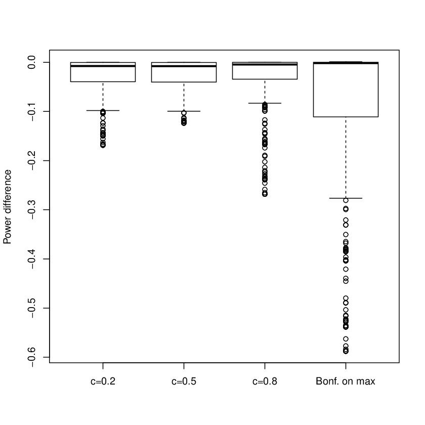
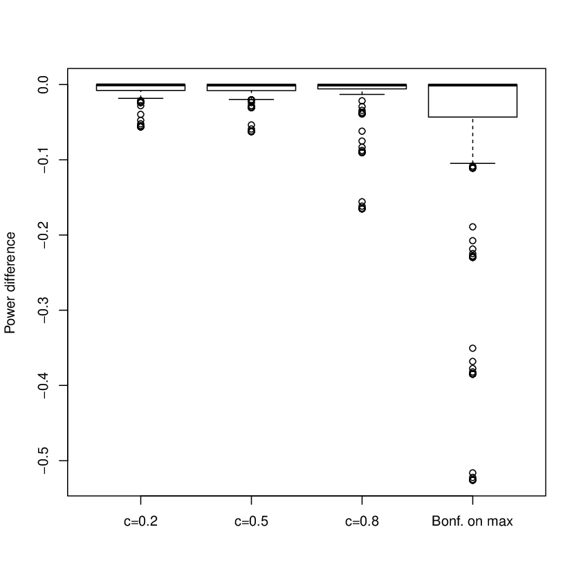
Figure 6 shows the difference in power of Procedure 3.1 using Bonferroni with , as well as the Bonferroni procedure on maximum -values, from the power of Procedure 3.1 with optimal choice of . Clearly, Procedure 3.1 with optimal choice of can be much more powerful than the Bonferroni procedure on maximum -values. Moreover, for the three choices , and , the difference in power from the optimal power is fairly small, especially when the optimal power is above 0.9 (right panel). Figure 7 shows the power as a function of for three configurations of , for which the power using the optimal is 0.9. The power function is quite flat. The optimal is below 0.5 in the top left panel, and above 0.5 in the top right and bottom panel. However, the difference in power between Procedure 3.1 with and Procedure 3.1 with optimal is small.




Appendix F Proof of Theorem 3.3
We use the notation given in the first two paragraphs of Appendix A of the main manuscript, including: is the indicator of whether was rejected for , and . In addition we define: is the set of hypotheses selected for follow-up based on .
Lemma F.1.
Assume that the -values across studies are independent, and the set of -values within the follow-up study has property PRDS. Then for any valid selection rule, the following results hold:
- 1.
Given for
- 2.
For Procedure 3.2 with parameters ,
- 3.
Item 2 holds if in the terms and in step 2 of Procedure 3.2, is replaced by for any value of
See Section F.1 for a proof.
Proof of item 1 of Theorem 3.3. We will first show that the first term of the sum in (A.1) is bounded by We will use the technique developed in Benjamini and Yekutieli, (2001) in the proof of their Theorem 1.3. For each and let us define:
Since is the entire sample space represented as a union of disjoint events, we obtain for each and :
| (F.1) |
Note that for for all , in particular Therefore, for each and
| (F.2) |
The upper bound on the first term of the sum in (A.1) is derived as follows.
| (F.3) | ||||
| (F.4) | ||||
| (F.5) |
where the first equality in (F.4) follows from (F.2), and the equality in (F.5) follows from (F.1). Note that for each
| (F.6) | ||||
| (F.7) |
The inequality in (F.6) follows from the fact that for for all Combining (F.7) with (F.5) we obtain an upper bound for the first term of the sum in (A.1):
| (F.8) |
It follows from Lemma F.1, item 3, that the second term of the sum in (A.1) is bounded by hence
Proof of item 2 of Theorem 3.3. We will first prove that the first term of the sum in (A.1) is bounded by For as defined in item 2 of Theorem 3.3, we denote The first term of the sum in (A.1) is upper bounded by two terms:
| (F.9) | ||||
| (F.10) |
where the inequality in (F.9) follows from the fact that yields that We will now find an upper bound for each of the two terms in (F.10) separately. The derivation of the upper bound for the first term is along the lines of the derivation in the proof of item 1. We give it below for completeness.
For each and let us define:
| (F.11) |
As in expression (F.2), for each and one has:
Using this equality we obtain:
| (F.12) |
Since is a union of disjoint events, we obtain for each and :
Therefore for each we obtain:
| (F.13) |
The inequality in (F.13) follows from the fact that for for all Combining (F.13) with (F.12) we obtain an upper bound for the first term of the sum in (F.10):
| (F.14) |
We will now find an upper bound for the second term of the sum in (F.10):
| (F.15) | ||||
| (F.16) | ||||
| (F.17) |
The inequality in (F.15) follows from the fact that for for all The inequality in (F.16) follows from the fact that for all it holds that yielding that The equality in (F.17) follows from the fact that is a union of disjoint events.
Combining (F.10), (F.14) and (F.17) we obtain an upper bound for the first term of the sum in (A.1):
| (F.18) |
Note that for therefore . We obtain which yields that in this case no modification is required.
It follows from Lemma F.1, item 3, that the second term of the sum in (A.1) is bounded by Combining this result with (F.18), we obtain
F.1 Proof of Lemma F.1
Proof of item 1. Our proof is similar to the proof of Theorem 1.2 in Benjamini and Yekutieli, (2001). For and we define the event as follows:
and we define to be the entire sample space of Note that It is easy to see that is the event in which if is rejected by Procedure 3.2, at most hypotheses are rejected including .
We will first show that for each , and is an increasing set for i.e. if and then The result follows from the fact that for fixed and for and is increasing in for
For a given and , using the fact that for each is an increasing set for as well as the PRDS property of the -values from the follow-up study and the independence of the -values across the studies, we obtain for each :
| (F.19) |
Using the fact that for each where and are disjoint events, and the fact that we obtain:
| (F.20) | ||||
Proof of item 2. Let be arbitrary fixed. Then,
| (F.21) | ||||
| (F.22) |
The first inequality in (F.22) follows from the independence of the -values across the studies and the fact that for each for all The second inequality in (F.22) follows from Lemma F.1, item 1. Taking the expectation over we obtain
Proof of item 3. For and arbitrary fixed,
The arguments that lead from (F.21) to the result of item 2 complete the proof.
Appendix G Additional theoretical results under dependence
Theorem G.1.
Assume that the -values across studies are independent, the -values within the primary study are independent, and the set of -values within the follow-up study has property PRDS. If the selection rule used in step 1 of Procedure 3.2 is a valid selection rule, then Procedure 3.2 with parameters controls the FDR at level for the family of no replicability null hypotheses .
Proof.
Let us first find an upper bound for the first term of the sum in (A.1). Note that (A.3) is established using the independence of the -values within the primary study only, therefore it holds for any form of dependence among the -values within the follow-up study. In particular, (A.3) holds under the dependency of Theorem G.1, establishing an upper bound for the first term of the sum in (A.1). It follows from Lemma F.1, item 2, that the second term of the sum in (A.1) is bounded by Thus we obtain:
Theorem G.2.
Assume that the -values across studies are independent. Then Procedure 3.2 with parameters controls the FDR at level for the family of no replicability null hypotheses if the selection rule used in step 1 of Procedure 3.2 is a valid selection rule, and the expressions in step 2 of Procedure 3.2 are modified as follows:
- 1.
In the terms and is replaced by , and in the terms and is replaced by .
- 2.
In the terms and is replaced by , and in the terms and is replaced by where
if only hypotheses with primary study -values at most a fixed threshold are considered for follow-up, i.e. .
Proof of item 1. We will first show that the first term of the sum in (A.1) is bounded by The first term of the sum in (A.1) equals to:
Now it follows from the arguments that lead from (F.3) to (F.8) that the first term of the sum in (A.1) is bounded by
Let us now find an upper bound for the second term of the sum in (A.1). For each and let us define:
| (G.1) |
Note that for each and :
| (G.2) |
The equalities follow from the fact that given is the whole sample space for , represented as a union of disjoint events. In addition, note that for each and
| (G.3) |
since for for all in particular Therefore, for each
| (G.4) | ||||
| (G.5) |
where the first inequality in (G.4) follows from (G.3), the next to last equality follows from (G.2), and the equality in (G.5) follows from the independence of the -values across the studies. Using similar arguments to those leading to (F.7), we obtain:
Combining this result with (G.5) we obtain for each :
It follows that
| (G.6) |
Using this fact and the upper bound for the first term of the sum in (A.1), we obtain that
Proof of item 2. The first term of the sum in (A.1) equals to:
Now it follows from the arguments that lead from (F.9) to (F.18) that the upper bound for the first term of the sum in (A.1) is
The second term of the sum in (A.1) is For each
where is defined in (G.1). Now it follows from the arguments that lead from (G.4) to (G.6) that the second term of the sum in (A.1) is bounded by Therefore,
Consider now a situation where both studies are available before the analysis, as described in Section 4 of the main manuscript. Without loss of generality, we label the studies as study one and study two.
Theorem G.3.
Assume the -values across studies are independent. Procedure 4.1 with parameters controls the FDR at level for the family of no replicability null hypotheses in either one of the following situations:
- 1.
The set of -values within each study has property PRDS, and the selection rule in step 1 of Procedure 3.2 is Bonferroni at level when the primary study is study one, and at level when the primary study is study two.
- 2.
Arbitrary dependence among the -values within each study, and the expressions in step 2 of Procedure 3.2 are modified as follows: in the terms and is replaced by and in the terms and is replaced by
Proof.
The proof of Theorem 4.1 in Appendix C relies only on the facts that Procedure 3.2 used in step 1 and in step 2 of Procedure 4.1 is valid. Therefore, the same proof shows that item 1 follows from item 2 of Theorem 3.3, and item 2 follows from item 1 of Theorem G.2.