Discrimination of models including doubly charged scalar bosons
by using tau lepton decay distributions

In this section, we review the polarization dependence of decays of $\tau$’s, and discuss how that could be traced in the case of $H^{\pm\pm}$ decay through $\tau$’s. In the following discussion, we assume that the leptonic decays of doubly charged scalar bosons occur via the Yukawa interactions, e.g., $H_{X}^{--}\overline{\ell_{X}}(\tau_{X})^{c}$ ($X=L,R$), where $H_{L}^{--}(H_{R}^{--})$ denotes $H^{--}$ only with the left-handed (right-handed) interaction. Hereafter, $\ell$ denotes $e$ or $\mu$.

First, let us consider the lepton flavor violating (LFV) decay $H^{--}\to\ell^{-}\tau^{-}$ followed by $\tau^{-}\to\pi^{-}\nu$. The branching ratio of the pionic decay of $\tau$ is about 11 % while the branching ratio of the total hadronic decay is about 65 %. The invariant-mass of $\ell\pi$ is expressed as $M^{2}_{\ell\pi}=z\,m_{H^{\pm\pm}}^{2}$ in the collinear limit, where $m_{H^{\pm\pm}}$ is the mass of $H^{\pm\pm}$ and $z\equiv E_{\pi}/E_{\tau}$; the $E_{\pi}$ and $E_{\tau}$ are energies of a pion and a $\tau$ lepton in the laboratory frame, respectively. This relation between the invariant-mass and the energy fraction is a good approximation for an energetic $\tau$ lepton, e.g., a $\tau$ lepton produced by a heavy particle decay.

The distributions of the pion energy fraction $z$ (namely, of the invariant-mass $M^{2}_{\ell\pi}$) are given as

where $F_{L,R}^{\pi}(z)$ are the fragmentation functions of $\tau^{-}_{L,R}\to\pi^{-}\nu$ decay in the collinear limit [19]. The fragmentation functions for the other hadronic decay modes are also known but less sensitive to the polarization of $\tau$ [19]. We will utilize these decay modes in the simulation study later.

When the LFV decay is followed by the leptonic decays of $\tau$’s, the dilepton invariant-mass is expressed as $M^{2}_{\ell\ell_{\tau}}=z\,m_{H^{\pm\pm}}^{2}$ in the collinear limit, where $z$ is the energy fraction of the daughter lepton to the parent $\tau$ lepton. We denote $\ell^{\pm}_{\tau}$ as $\ell^{\pm}$ from decays of $\tau^{\pm}$.²² 2 The notation $\ell_{(\tau)}\ell_{(\tau)}$ indicates not only $ee$ and $\mu\mu$ but also $e\mu$. The total branching ratio of the leptonic decays is about 35 %. The distributions of $z$ (namely, of $M^{2}_{\ell\ell_{\tau}}$) are given as

where $F_{L,R}^{\ell}(z)$ are the fragmentation functions of $\tau_{L,R}^{-}\to\ell_{\tau}^{-}\nu\bar{\nu}$ decay in the collinear limit [19].

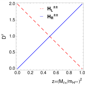
In Fig. 1, we plot the distributions of the invariant-masses of $\ell\pi$ (left panel) and $\ell\ell_{\tau}$ (right panel) for the LFV decay $H^{--}\to\ell^{-}\tau^{-}$ followed by the pionic and leptonic decays of the $\tau$, respectively. The invariant-mass distributions via the decay of $\tau_{L}$ ($\tau_{R}$) are plotted in the dashed (solid) curves. For the pionic decay channel, the distributions are linear in $z$ and have an opposite behavior between $\tau_{L}$ and $\tau_{R}$. On the other hand, the right panel of Fig. 1 shows that the distribution of $M_{\ell\ell_{\tau}}$ for the leptonic $\tau$ decay would be less sensitive to the $\tau$ polarization than that of the pionic channel.

Next, we consider the decay mode $H^{--}\to\tau^{-}\tau^{-}$. The decay pattern of the two $\tau$’s can be classified into three categories: hadronic channels (e.g. $\pi\pi$), semi-leptonic channels (e.g. $\ell_{\tau}\pi$), and purely leptonic channels ($\ell_{\tau}\ell_{\tau}$). The distributions of $\pi\pi$ invariant-mass $M_{\pi\pi}$ in $H^{--}\to\tau^{-}\tau^{-}\to\pi^{-}\pi^{-}\nu\nu$ decay chain are calculated by convoluting the fragmentation functions of the pionic decays of $\tau$’s in Eqs. (4) as follows [21]:

where $z=M^{2}_{\pi\pi}/m_{H^{\pm\pm}}^{2}$ in the collinear limit and ${\cal D}^{\pi\pi}_{LL}$ (${\cal D}^{\pi\pi}_{RR}$) is the distribution for $H^{\pm\pm}_{L}$ ($H^{\pm\pm}_{R}$).

The distributions of the $\ell_{\tau}\pi$ invariant-mass $M_{\ell_{\tau}\pi}$ for the $H^{--}\to\tau^{-}\tau^{-}\to\ell_{\tau}^{-}\pi^{-}\nu\nu\bar{\nu}$ decay chain are given by

where $z=M^{2}_{\ell_{\tau}\pi}/m_{H^{\pm\pm}}^{2}$ in the collinear limit. The distribution ${\cal D}^{\ell\pi}_{LL}$ (${\cal D}^{\ell\pi}_{RR}$) is for $H^{\pm\pm}_{L}$ ($H^{\pm\pm}_{R}$).

The dilepton invariant-mass distributions for the $H^{--}\to\tau^{-}\tau^{-}\to\ell_{\tau}^{-}\ell_{\tau}^{-}\nu\nu\bar{\nu}\bar{\nu}$ decay chain are given by

where $z=M^{2}_{\ell_{\tau}\ell_{\tau}}/m_{H^{\pm\pm}}^{2}$ in the collinear limit and ${\cal D}^{\ell\ell}_{LL}$ (${\cal D}^{\ell\ell}_{RR}$) is for $H^{\pm\pm}_{L}$ ($H^{\pm\pm}_{R}$).

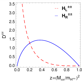
In Fig. 2, we plot the distributions of the invariant-mass of $\pi\pi$ (left panel), $\ell_{\tau}\pi$ (middle panel), and $\ell_{\tau}\ell_{\tau}$ (right panel) from $H^{--}\to\tau^{-}\tau^{-}$. The invariant-mass distributions through the decay of $\tau_{L}$ ($\tau_{R}$) are plotted in the dashed (solid) curves. Owing to the large polarization dependence of the pionic decay fragmentation function in Eqs. (4), the $\pi\pi$ invariant-mass distribution has a large power for the spin analysis. Namely, the distribution takes a large value in the region of a small $z$ for the $H_{L}^{\pm\pm}$ decay while it is large for $z\simeq 0.4$ in the $H_{R}^{\pm\pm}$ decay. The $\ell_{\tau}\pi$ and $\ell_{\tau}\ell_{\tau}$ distributions in the middle and right panels of Fig. 2, respectively, take a large value for a small $z$ for both $H_{R}^{\pm\pm}$ and $H_{L}^{\pm\pm}$, thus are not useful as the $\tau$ polarization discriminator.

To summarize, the invariant-mass distributions of $\ell\pi$ (and $\ell\ell_{\tau}$) in the $H^{--}\to\ell^{-}\tau^{-}$ decay and $\pi\pi$ in the $H^{--}\to\tau^{-}\tau^{-}$ decay are good for discriminating the $\tau$ polarization and thus the chiral structure of the Yukawa interaction with $H^{\pm\pm}$. Notice that the $\ell\pi$ ($\ell\ell$) final-state can be reached through the other decay chain(s) such like $H^{--}\to\tau^{-}\tau^{-}\to\ell_{\tau}^{-}\pi^{-}\nu\nu\bar{\nu}$ ($H^{--}\to\ell^{-}\ell^{-}$ and $H^{--}\to\tau^{-}\tau^{-}\to\ell^{-}_{\tau}\ell^{-}_{\tau}\nu\nu\bar{\nu}\bar{\nu}$). If these decay modes for $H^{\pm\pm}$ exist simultaneously, the signatures from these decay chains would mix in general. It should be possible to treat the mixed signatures or to divide them by kinematical cuts. However, since such analyses depend on the detail branching ratio of the $H^{\pm\pm}$ decay, we will not consider them in this study.

In order to perform realistic studies for collider experiments, we examine a Monte-Carlo simulation for the $H^{++}H^{--}$ pair production and their decays up to parton-showering and hadronizations. We generate signal events of $pp\to H^{++}H^{--}$ by using Pythia [25] with handling the $\tau$ decay by TAUOLA [26] incorporating the chiral properties of the Yukawa interactions of $H^{\pm\pm}$. We consider only the leptonic decay of $H^{\pm\pm}$, and pick up several patterns of the pair of decays suited for the $\tau$ polarization measurement. The $m_{H^{\pm\pm}}$ is set to be $400\,{\text{GeV}}$, and the collider energy to $\sqrt{s}=14\,{\text{TeV}}$. For the reference, the $H^{++}H^{--}$ production cross-sections is 4.6 fb for the HTM and 1.9 fb for the ZBM. For the analysis, we use lighter leptons ($e$ and $\mu$) with $p_{T}^{\ell}>15\,{\text{GeV}}$ and $|\eta_{\ell}|<2.5$, where $p_{T}$ is the transverse momentum and $\eta$ is the pseudo rapidity. To find the hadronically decaying $\tau$’s, we perform $\tau$-tagging for every jets with $p^{j}_{T}>25\,{\text{GeV}}$ and $|\eta_{j}|<2.5$ which are constructed by the anti-$k_{T}$ algorithm [27] with $R=0.4$. For the $\tau$-tagging, we use two methods. The first method is devoted to extract the $\tau\to\pi\nu$ decay. Namely, it is tagged as the pionic $\tau$-jet ($\pi_{\tau}$) if a jet has only 1 charged hadron and its transverse energy dominates more than 0.95 of the jet. The second method is a more general-purpose; we define $j_{\tau}$ as a jet which contains 1 or 3 charged tracks in a small cone ($R=0.15$) centered at the jet momentum direction with the transverse energy deposit to this small cone more than 0.95 of the jet. The second method could tag the $\tau$ decay into $2\pi$ and $3\pi$ originated from $\tau\to\rho\nu$ and $a_{1}\nu$ decays, in addition to the single $\pi$. Thus the tagging efficiency is better than the first method, but the spin analysis power is weakened.

The extensive signal-to-background studies including $\tau$’s can be found, for example, in Ref. [13, 14]. Following their results, a clear signal extraction is expected by the requirement of the same-signed dilepton and possibly a peak in their invariant-mass. Thus, we present the simulation results only for the signal events, but not for the background events. Expected background processes are diboson production, $t\bar{t}$ plus one boson production, etc.

As the first case, we deal with $pp\to H^{++}H^{--}\to\ell^{+}\ell^{+}\ell^{-}\tau^{-}$. This decay pattern can be easily identified by requiring the same-signed dilepton with a sharp peak in their invariant-mass distribution. The mass of $H^{\pm\pm}$ can be clearly obtained from the peak. Then, the invariant-mass distribution of the remaining $\ell^{-}$ and decay products of $\tau^{-}$ can be used for the polarization discriminant. We take the hadronic decays of $\tau$, because of the better spin analysis power than the leptonic ones as shown in Fig. 1.

In Fig. 3, the invariant-mass distributions of $\ell\pi_{\tau}$ (left panel) and those of $\ell j_{\tau}$ (right panel) from $H^{--}\to\ell^{-}\tau^{-}$ are shown for the events with $3\ell$ and one $\tau$-tagged jet. Results for the decay of $H_{L}^{\pm\pm}$ ($H_{R}^{\pm\pm}$) are plotted in the dashed (solid) histograms. The $y$-axis of the plots hereafter stands for the number of events in our simulation. For each of $H^{\pm\pm}_{L}$ and $H^{\pm\pm}_{R}$, we generate $3\times 10^{4}$ events of the $pp\to H^{++}H^{--}\to\ell^{+}\ell^{+}\ell^{-}\tau^{-}$ process followed only by hadronic $\tau$ decays. Corresponding integrated luminosity of our simulation depends on the branching ratio of $H^{\pm\pm}$, which however we don’t specify in this study. The signal selection efficiencies with the $\pi_{\tau}$ method and the $j_{\tau}$ method in Fig. 3 are about $13\%$ ($15\%$) and $62\%$ ($62\%$), for $H^{\pm\pm}_{L}$ ($H^{\pm\pm}_{R}$) events in our simulation, respectively.

The distributions in the left panel roughly reproduce the linear dependence on $z$ given in Eqs. (4) which are superimposed with some normalization. Thus, the pionic $\tau$-tagging method seems to be working well to catch the pionic $\tau$ decay products. The effect of the kinematical cuts can appear in the small $z$ region due to the $p_{T}$ cut. The discrimination of the two distributions may be possible with just a small number of events. When we employ the general $\tau$-tagging method, the expected number of events becomes 5 times larger than that for the case with pionic $\tau$-tagging method. Since the distributions for $H_{L}^{\pm\pm}$ and $H_{R}^{\pm\pm}$ still differ from each other, although the difference is weakened, this general $\tau$-tagging method works as well for our purpose. We note that the distributions in the right panel could be understood as the sum of the various hadronic $\tau$ decay contributions with proper polarization dependence [19]. The distributions are scaled by the mass of $H^{\pm\pm}$, thus it is expected that these distributions does not depend on the value of the mass so much. We have confirmed that quite similar distributions are obtained for the case with a heavier mass of $H^{\pm\pm}$.

The second case is $pp\to H^{++}H^{--}\to\ell^{+}\ell^{+}\tau^{-}\tau^{-}$. We note that this process can be useful when the branching ratio for the LFV decay $H^{--}\to\ell^{-}\tau^{-}$ is so small that we cannot use the first case ($H^{++}H^{--}\to\ell^{+}\ell^{+}\ell^{-}\tau^{-}$). This collider signature has also a sharp peak in the invariant-mass distribution of the same-signed dilepton, thus the signal event extraction from the background contributions would be easy. We analyze the case where both of $\tau$ leptons decay into hadrons because of the best spin analysis power as shown in Fig. 2.

In Fig. 4, the invariant-mass distributions of $\pi_{\tau}\pi_{\tau}$ (left panel) and those of $j_{\tau}j_{\tau}$ (right panel) from $H^{--}\to\tau^{-}\tau^{-}$ in the $pp\to H^{++}H^{--}\to\ell^{+}\ell^{+}\tau^{-}\tau^{-}$ process are shown. We generate $3\times 10^{4}$ events of the process followed only by the hadronic decays of $\tau$’s. Results for the decay of $H_{L}^{\pm\pm}$ ($H_{R}^{\pm\pm}$) are plotted in the dashed (solid) histograms. Distributions of Eqs. (6) are superimposed to the left panel with some normalization as references. As expected, behaviors of the distributions in the left panel are almost the same as Eqs. (6) even after the selection cuts. For the $j_{\tau}j_{\tau}$ invariant-mass distributions, the curves for $H^{\pm\pm}_{L}$ and for $H^{\pm\pm}_{R}$ are still well separated.

The third case is for a situation in which $H^{--}\to\ell^{-}\ell^{-}$ does not exist. Then the signature would be $pp\to H^{++}H^{--}\to\ell^{+}\tau^{+}\ell^{-}\tau^{-}$, which seems better than $pp\to H^{++}H^{--}\to\ell^{+}\tau^{+}\tau^{-}\tau^{-}$. The momentum reconstruction of the two $\tau$’s is still possible by using a collinear approximation for the decay of the two $\tau$’s [13]. Then the mass of $H^{\pm\pm}$ can be measured by the invariant-mass of the same-signed $\ell\tau$ pairs. If both of the $\tau$’s decay hadronically, we may suffer from the background contribution. In order to suppress the background contribution, we require that one $\tau$ decays leptonically which gives the same-signed dilepton $\ell\ell_{\tau}$. The hadronic decay for the other $\tau$ will be preferred for the discrimination of the polarization, although the $\ell^{+}\ell^{+}_{\tau}\ell^{-}\ell^{-}_{\tau}$ signature may be also exploited.

In Fig. 5, the invariant-mass distributions of $\ell\pi_{\tau}$ (left panel), those of $\ell j_{\tau}$ (middle panel) are shown for the event in which the momentum reconstruction is resolved by using the collinear approximation method.³³ 3 One may wonder how to select $\ell_{\tau}^{-}$ for the collinear approximation method under the existence of $\ell^{-}$. One can find the correct one which gives the smaller difference of the reconstructed invariant-masses of the two $\ell^{\pm}\tau^{\pm}$ pairs. We generate $3\times 10^{4}$ events of the $pp\to H^{++}H^{--}\to\ell^{+}\tau^{+}\ell^{-}\tau^{-}$ process. The decay of a tau lepton is not restricted to the hadronic ones in contrast with simulations for Figs. 3 and 4. The full momentum reconstruction is not necessary to obtain the plots in Fig. 5, but is very effective to extract the signal events of this decay pattern. Distributions of Eqs. (6) are superimposed to the left panel with some normalization as references. Behaviors of the obtained invariant-mass distributions of $\ell\pi_{\tau}$ and $\ell j_{\tau}$ are almost the same as those in the $pp\to H^{++}H^{--}\to\ell^{+}\ell^{+}\ell^{-}\tau^{-}$ process in Fig. 3. In addition, in the right panel, we plot the invariant-mass distributions of the same-signed $\ell\ell_{\tau}$ pair from the other side of the $H^{\pm\pm}$ decays. The behaviors of $\ell\ell_{\tau}$ invariant-mass distributions are in good agreement with Eqs. (5) whose distributions are superimposed with some normalization as references. Due to the good momentum resolution of leptons, the dilepton invariant-mass distributions could be also useful for the $\tau$ polarization discrimination.

Finally, we comment on the case where $H^{--}$ decays only into $\ell^{-}\ell^{-}$ or $\tau^{-}\tau^{-}$. If $H^{--}$ decays only into $\ell^{-}\ell^{-}$, it is impossible to observe any polarization phenomena from kinematical measurements. Then we should rely on predictions in each model about the $H^{\pm\pm}$ production cross-section and the decay branching ratios in order to distinguish models. If $H^{--}$ decays only into $\tau^{-}\tau^{-}$, $H^{++}H^{--}$ gives the $4\tau$ signature. Since, there are too many sources of the missing momentum, the momentum reconstruction for the $\tau$’s is not possible, we cannot use the invariant-mass peak at $m_{H^{\pm\pm}}$ for the background reduction. For the similar signatures in the context of the two Higgs doublet model, however, a sufficient background reduction is expected in the various channels for the $\tau$ decays [28]. Thus, the invariant-mass distributions, for example, in the $\ell^{\pm}_{\tau}\ell^{\pm}_{\tau}j_{\tau}j_{\tau}$ channel may be used for the polarization discriminant. Notice that the information on $m_{H^{\pm\pm}}$ could be obtained by the endpoint of the invariant-mass distributions [28].