Magnetic properties of nanoscale compass-Heisenberg planar clusters
Abstract
We study a model of spins on a square lattice, generalizing the quantum compass model via the addition of perturbing Heisenberg interactions between nearest neighbors, and investigate its phase diagram and magnetic excitations. This model has motivations both from the field of strongly correlated systems with orbital degeneracy and from that of solid-state based devices proposed for quantum computing. We find that the high degeneracy of ground states of the compass model is fragile and changes into twofold degenerate ground states for any finite amplitude of Heisenberg coupling. By computing the spin structure factors of finite clusters with Lánczos diagonalization, we evidence a rich variety of phases characterized by symmetry, that are either ferromagnetic, -type antiferromagnetic, or of Néel type, and analyze the effects of quantum fluctuations on phase boundaries. In the ordered phases the anisotropy of compass interactions leads to a finite excitation gap to spin waves. We show that for small nanoscale clusters with large anisotropy gap the lowest excitations are column-flip excitations that emerge due to Heisenberg perturbing interactions from the manifold of degenerate ground states of the compass model. We derive an effective one-dimensional XYZ model which faithfully reproduces the exact structure of these excited states and elucidates their microscopic origin. The low energy column-flip or compass-type excitations are robust against decoherence processes and are therefore well designed for storing information in quantum computing. We also point out that the dipolar interactions between nitrogen-vacancy centers forming a rectangular lattice in a diamond matrix may permit a solid-state realization of the anisotropic compass-Heisenberg model.
pacs
75.10.Jm, 03.65.Ud, 05.30.Rt, 64.70.TgI Introduction
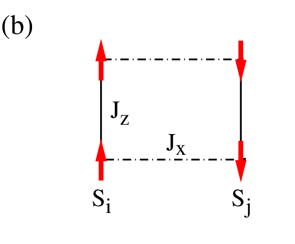
Frustrated quantum magnetism belongs to the very active research areas in condensed matter theory. Frustration is one of the simplest concepts in physics with far reaching consequences.[1, 2] It is well known that antiferromagnetic (AF) exchange for three spins on a triangle is geometrically frustrated, both in classical Ising and in quantum Heisenberg models. On a two-dimensional (2D) square lattice, frustration typically involves interactions between further neighbors competing with those between nearest neighbors, but it can also occur with only the latter ones: for instance when, compared to the Ising model, the sign of spin exchange along every second column is reversed. The resulting model, called fully frustrated Ising model, [3] is exactly solvable, with a phase transition at a lower temperature than that of the 2D Ising model [4] — the low temperature phase, with extensive entropy due to frustration, is described in terms of dimer coverings of the dual lattice.[5] A quantum analog of this classical frustrated model on a square lattice is the 2D quantum compass model (QCM),[6] where interactions couple either or components of nearest neighbor spins, depending on the spatial bond direction or respectively. When the associated exchange constants and [see Fig. 1(b)] have different values, these two spin components are nonequivalent. Yet even otherwise, and in spite of its dimensionality, this model displays a finite-temperature phase transition of the 2D Ising universality class, [7] but the symmetry broken phase at low temperature is characterized by high ground state degeneracy in the thermodynamic limit. [8]

One can interpolate between the 2D QCM and Ising models by modifying continuously the spin components coupled on the bonds along two distinct lattice directions.[9] This allows one to highlight that the QCM is closely related to orbital physics, where the exchange interactions are directional.[10] In fact, one finds a 2D superexchange model for orbitals as an intermediate model when the interactions are gradually modified from the classical Ising model toward the QCM. While the frustration of interactions is clearly weaker in the orbital model than in the QCM, the latter may be considered as a generic description of frustrated directional orbital interactions which arise for strongly correlated electrons in transition metal oxides with partly filled degenerate orbitals, and is realized for instance in manganites.[11] In these systems the orbital degrees of freedom play a crucial role in determining ground states with coexisting magnetic and orbital order, described by spin-orbital superexchange. [12, 13, 14, 15, 16, 17, 18]
The orbital interactions are intrinsically frustrated [13] as they have low symmetry in pseudospin space representing the orbital degrees of freedom. Typically the symmetry is that of the lattice due to the shape of wave functions, and not the SU(2) symmetry typical for spin exchange interactions. Although frustration is at its maximum in three-dimensional (3D) models and it was concluded from the high-temperature expansion that a phase transition to the symmetry-broken states does not occur,[19] recent Monte-Carlo simulations have evidenced symmetry-broken phases at low temperatures both in and orbital models.[20, 21] This contrasts with a formal analog of the QCM defined on the honeycomb lattice, the Kitaev model,[22] for which an exact solution evidenced a spin liquid ground state. In fact, both models can describe orbitally degenerate Mott insulators in the limit of strong spin-orbit coupling [23] which selects a low-energy doublet at each transition metal ion represented by a pseudospin- variable — which model is actually relevant depends on the geometry of the system. However, realistic orbital models are more involved,[10] inter alia due to non-conservation of the orbital quantum numbers that follows both from hybridization processes with oxygen orbitals in an oxide and from the structure of charge excitations controlled by Hund’s exchange in orbital degenerate systems. The QCM was designed to avoid all these complications and to address a paradigm of intrinsic frustration due to directional conflicting interactions.
Another motivation for introducing and investigating the 2D QCM comes from the field of quantum computing.[24, 25] Recent progress includes proposals for the optimal choice of protected qubits.[26] Several realizations of computing devices with protected qubits have been proposed in various contexts: (i) in Josephson junction arrays,[27, 28] as well as (ii) with polar molecules, or (iii) with systems of trapped ions in optical lattices.[29] In all these cases the QCM provides the generic description of interacting spins.
In general, in order to construct a device which could serve for information storage, a manifold of degenerate states is required, [30] and these degeneracies should be stable against noise and other small perturbations[27] thanks to particular symmetries of the Hamiltonian. This is actually the case in the quantum compass model, where two types of symmetry operations described by operators and commute with the Hamiltonian but not with each other, see Sec. II. As a result the eigenstates of the system are characterized by related integrals of motion, and concerning the ground state, by a hidden dimer-dimer symmetry.[31] More importantly, an exact twofold degeneracy of all quantum levels was evidenced on finite clusters of arbitrary size, being of advantage for quantum information.[27] These degeneracies are, thanks to the non-local nature of operators and , robust to local perturbations; in consequence qubits defined by a realization of the QCM are expected to be protected against noise, so that this model is of prime interest for quantum computing.
The QCM has thus an interdisciplinary character as it plays an important role in the modeling not only of correlated transition metal oxides, but also of protected qubits for quantum computations. An intriguing question important in all these contexts and asked shortly after the QCM was introduced concerns the nature of a quantum phase transition (QPT) that occurs when anisotropic interactions are varied through the isotropic point, also called the compass point. A first order transition between two distinct phases with directional ordering, along either rows or columns, was suggested by Lánczos diagonalization and Green’s function Monte-Carlo simulations for finite clusters,[8] and later confirmed using a projected entangled-pair state algorithm.[32] At this transition, a discrete symmetry in spin space is spontaneously broken since the frustrated interactions along two different directions are equivalent and the spin orientation follows one of them. In terms of broken symmetries this transition is remarkably similar to the first order QPT found at in the exact solution of the one-dimensional (1D) QCM, [33] or a compass ladder,[34] where two different types of order stem from the invariant subspaces of the 1D model. This suggests that a similar mechanism may operate also in two dimensions.
Particularly in the context of proposed realizations of quantum computing devices based on finite clusters with compass-like spin interactions, a fundamental question to ask is how the highly degenerate ground states [8] are modified when a small perturbation occurs. We argue that Heisenberg interactions between nearest neighbor spins stand for a class of perturbations to the compass terms which are typical in solid state systems — for instance a Hamiltonian with compass and Heisenberg terms would describe exchange processes in some Mott insulators with strong spin-orbit coupling and 180-degree bonds. [23] In a broader perspective we study in this work the effect of Heisenberg perturbations, by considering a generalization of the QCM called the compass-Heisenberg (CH) model.[35]
We find that the high degeneracy of ground states in the thermodynamic limit (TL) is removed by Heisenberg terms of arbitrarily small amplitude, and various magnetically ordered phases arise, with a preferred spin direction related to the ordered pattern. In macroscopic systems the lowest energy excitations are thus gapped spin waves; on nanoclusters however, for small enough Heisenberg amplitude, another type of excitations can be of lower energy than spin waves: these are the column-flip excitations, from the ordered ground states selected by small Heisenberg terms to the many other eigenstates of the low-energy manifold minimizing the energy of dominating compass interactions. The column-flip excitations are robust with respect to decay into spin waves, and preserve an original multiplet structure which can be captured by an adapted effective model; this analysis leads us to propose that these excitations could be used in a novel type of solid-state-based quantum computing scheme in a regime of moderate Heisenberg interactions.
In particular we find in the frame of the CH model that the compass point (, ) appears as a quadri-critical point where four distinct phases with symmetry meet in the plane spanned by two parameters, and , characterizing the compass- and the Heisenberg couplings. We note that the transitions between arbitrary two phases and related by a duality transformation are continuous transitions for finite system size, while they appear as first order transitions in the TL.[32] Here we find that also the transitions between phases and belonging to distinct symmetries show a similar behavior. Remarkably, these transitions are characterized by the softening of certain columnar excitations rather than of spin waves.
Recent experimental developments on arrays of nitrogen-vacancy (NV) centers, constituting point-like defects in a diamond matrix, [36, 37] may bring a further motivation to the study of a model with coexisting compass and Heisenberg interactions. Indeed these defects can be effectively described by quantum spins ,[38] coupled (under certain conditions) predominantly by the dipolar interactions [39] of the form:
| (1) |
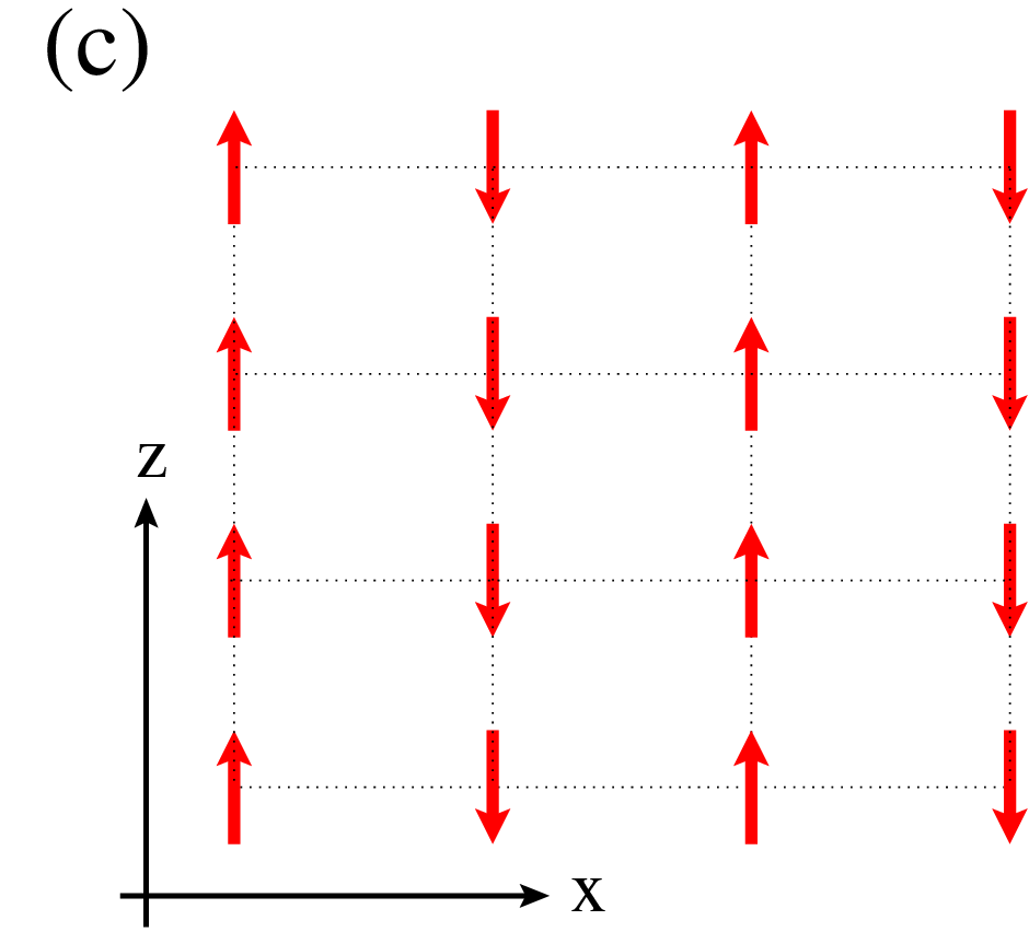
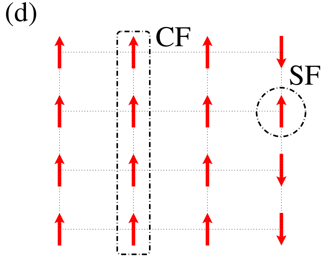
where the axis in spin space is along the spatial direction connecting spins and . These interactions are long-ranged, but rapidly decaying with distance; if defects sit on sites of a rectangular cluster, the (dominant) interactions between nearest neighbors are a sum of Heisenberg-like and compass-like terms.[35] Beyond the nature of couplings, an aspect which must be taken into consideration in this context is a possible splitting of energy levels for a single NV center. One can a priori consider a situation where these splittings are small before the typical energy scale of dipolar couplings; alternatively, other possible realizations of dipolar-coupled spin arrays are conceivable (with e.g. nuclear spins, in a layered crystal with an orthorhombic unit cell and negligible effects of hyperfine coupling to electron spins). We will show below that in such systems the lowest energy excitations can consist of reversing entire columns of spins, and these could be used for encoding protected qubits, see Fig. 1.
The paper is organized as follows. In Sec. II we introduce the CH model and state the problem of frustrated interactions and possible QPTs. There are two variants: the ferromagnetic (FM) and the antiferromagnetic (AF) CH model. We first focus on the AF CH model, and present selected data for the spin structure factors in Sec. III and show that long-range order is induced by arbitrarily small Heisenberg interactions. The full phase diagram of the CH model is presented in Sec. IV — there, we provide evidence that some phase transitions occur for the same interaction parameters as in the classical CH model, while other transition lines are affected by quantum fluctuations, see Secs. IV.2.1 and IV.2.2. Next we analyze the features of the FM CH model and discuss its phase diagram in Sec. IV.3. Spin wave excitations are derived and discussed for different phases in Sec. V. We turn then to the analysis of the lowest energy states of finite clusters and show in Sec. VI that: (i) the ground state and the low energy excitations are very well described by an effective 1D model which captures the essential parameter dependence of columnar (i.e., column-flip) excitations characteristic of the compass-Heisenberg model; and (ii) there exists a parameter range where the column-flip excitations are the lowest energy excitations and cannot decay into spin waves. The paper is summarized in Sec. VII, where open issues and possible extensions of this work are also discussed.
II Compass-Heisenberg model
We consider a model of spins on the square lattice, with axes in the plane, labeled here and after the interacting spin components in the QCM. The nearest neighbor interactions are of two types: (i) frustrated compass interactions of amplitudes and , and (ii) Heisenberg interactions with an exchange . While the Heisenberg interaction is isotropic in spin space and bond-independent, the compass interactions depend on the bond direction. On bonds along the -axis the -components of spins are coupled by terms (we label the sites in a 2D cluster by two indices ), and on bonds along the -axis the coupling concerns the -components, being of the form . For convenience we use here Pauli matrices with such that in the basis.
The CH Hamiltonian reads: [35]
| (2) | |||||
Here the sums over and run over the intervals and consistent with either periodic boundary conditions (PBC) or open boundary conditions (OBC). We consider rectangular clusters with spins and for both PBC and OBC. Another type of clusters (considered only with PBC) are clusters tilted by w.r.t. the previous ones and containing spins (for ).[40]
The structure of eigenstates of depends only on the relative amplitude of parameters , and in Eq. (2). Thus, the total space of interaction parameters may be characterized by a point on the spherical surface parametrized by angles , see Fig. 2. The compass interactions are then described by the related global interaction strength,
| (3) |
and the angle determines the exchange constants,
| (4) |
that are represented by a point in the plane, see Fig. 3. Using this parametrization the Heisenberg interaction is given by the angle :
| (5) |
In the following we shall denote by antiferromagnetic compass-Heisenberg (AF CH) model the case where , and by ferromagnetic compass-Heisenberg (FM CH) model the case .

We introduce certain non-local operators playing a central role in the QCM (and, as we will see, in the CH model), and defined either on rows or on columns of the considered clusters, by:
| (6) | |||
| (7) |
Here rotates all spins in the column from up- to down-orientation or vice versa — this operation is called column flip (CF), see Fig 1(d). Similarly, rotates a whole row of spins pointing along direction into direction in spin-space. In the QCM () these operators are known [8, 27] to commute with the compass Hamiltonian (i.e., , ) and — restricting now to the first type of (untilted) clusters — they anticommute (), accounting for an exact twofold degeneracy.

In presence of Heisenberg interactions, the commutators above become non-zero. To evaluate those, it is useful to consider separately two terms , complementary to each other in Eq. (2): the first term acts on horizontal bonds (rows), while the second term acts on vertical bonds (columns). It is now straightforward to show that commutes with the columnar interaction, i.e., , but not with the Heisenberg interactions on the rows
| (8) |
Hence the column is here coupled to the left () and the right () column by and components of Heisenberg interactions.
These operators are related to a formalism which allows one to understand the high ground state degeneracy of the QCM in the TL, and which we will briefly describe here. We consider a situation with strong anisotropy , which calls for a perturbative treatment of couplings. The unperturbed Hamiltonian contains only the compass couplings, which select, on a rectangular cluster, columnar states. These states, where in each column all spins point along the same axis — aligned either ferromagnetically or antiferromagnetically depending on the sign of —- can be labeled using pseudospin variables , with . For a given columnar state, a given column will be described by an eigenstate of the pseudospin operator , either or , depending on whether the spin at a reference site has the orientation up or down respectively; orientations of other spins in the column follow from its FM () or AF () long-range ordered nature. In both cases, the operators and flip all spins of the column with amplitudes given by the respective Pauli matrices. The operator has actually the same action on a column as the operator , with the only difference that is defined only in the subspace generated by columnar states. The action of operators on a reference columnar state defines column-flip excitations, which will be analyzed in Sec. VI and correspond qualitatively to flipping all spins in a column of a finite cluster [see Fig. 1(d)]. They are well defined when perturbing interactions favor a particular columnar pattern in the ground state, and we will see that this is typical for the CH model.
Within the QCM (for ), the perturbation theory describing the effects of small couplings acts in the subspace of columnar states.[27] We recall the expression of the effective Hamiltonian obtained at leading order: [27, 8]
| (9) |
Here the effective coupling constant describing the flip of a whole column is obtained at order in perturbation theory:
| (10) |
The coefficient depends on boundary conditions (with or without a prime for OBC or PBC, respectively) and on the column length; it can be determined by considering all processes flipping two neighboring columns and , by successive actions of perturbing terms .
Assuming PBC, the excitation energies of intermediate states during such -th order processes are integer multiples of the quantity which appears in Eq. (10). The counting of these processes, weighted by a factor depending on the excitation energies at each step of each process, is a combinatorial problem which, to our knowledge, does not have a general analytic solution; however for small the exact values of , or equivalently of , are easily computable. As examples we give here , and . In the case of OBC, the number of processes flipping two neighboring columns of sites is the same as for PBC, but the excitation energies at some intermediate steps may be lower than in the periodic case so that , e.g. for one has . One can even remark that with PBC , by noticing that there are exactly column-flipping processes for which the excited energy at each step is minimal, i.e., (these are the processes where two successive actions of perturbing terms occur on bonds distant by 1 unit along the axis).
A scaling law for the size-dependence of , or equivalently of , was given in Ref. 8, indicating that the latter vanishes exponentially with increasing — in the compass model with this yields precisely the -fold ground state degeneracy in the TL. The isotropic case has a higher ground state degeneracy in the TL, which can be deduced from similar arguments.
As mentioned before, the compass model itself is characterized by a high level of frustration between and interactions, independent of the sign of the associated amplitudes. From that perspective, the introduction of perturbing Heisenberg interactions seems to increase the degree of frustration in the model, e.g. in a case where they are of sign opposite to that of dominant compass interactions. The ordered patterns favored in this case, if ever, are expected to differ from those selected for dominant Heisenberg interactions, i.e., - in the former case, a ground state minimizing energy both of dominant compass interactions (on either vertical or horizontal bonds, depending on the sign of ) and of Heisenberg interactions (on other bonds) can be selected; while in the latter, a FM or Néel order is expected with an easy axis selected by compass couplings. Thus, besides the question of whether the exotic, semi-disordered ground states characteristic of the compass model can actually exist in presence of Heisenberg couplings with small amplitudes, one can focus in this model on the determination of the phase diagram, with multiple phase transitions between the more conventional FM or Néel phases, and more exotic -type AF phases, with FM order along one axis and AF along the other. The characterization of these phases is the subject of the next chapter.
III Spin structure factors
In this Section we address the following central question: What happens to the macroscopic -fold ground-state degeneracy of the anisotropic QCM in the presence of Heisenberg perturbations? We show that in the most general case, where compass coupling strengths and are not equal and where the Heisenberg coupling strength is finite, the ground state is characterized by long-range spin order with a certain easy axis. This is evidenced by spin structure factors , defined for each orthogonal spin component as:
| (11) |
For given interaction parameters, a peak in at a single momentum and component signals an ordering of spins with a finite component along the axis and a modulation period given by .

Let us exemplify this in a situation where all couplings are AF, and , see Fig. 4. The large peak of found at for indicates that the corresponding ground state is of the type, that is Néel-ordered with spins along the axis. We encountered similar ordering features for varying from very small to very large values, keeping the compass amplitudes fixed such that . In the limit, this can be interpreted as follows: small compass couplings break the symmetry of Heisenberg interactions and select an easy axis for the Néel order; it is obvious here that this easy axis is . In the limit , the selection of order is to be understood differently: we recall that compass couplings alone, on a cluster, select a class of columnar states, characterized by long-range Néel-type correlations along columns but short-range correlations along rows. These states are separated from higher energy levels by a large gap which is in the Ising limit .
This semi-ordered nature of the GS is reflected in Fig. 4(a) for by a structure factor spread over all momenta of the form — for , one would indeed have . The effect of small compass couplings is mostly to reduce slightly the difference of at and , respectively. In contrast, even very small Heisenberg couplings have a much stronger effect, seen in the example of Fig. 4: they result in a strong enhancement of , compared to for . The fact that this enhancement is much stronger in this case for , than in the anisotropic case for of Fig. 5(c), can be understood within the effective pseudospin model which we will describe in Sec. VI.1. To explain this, we notice that the columnar states include two Néel-like states, where spins on each -oriented bond connecting neighboring columns are antiferromagnetically arranged. These states are favored over the other columnar states by AF Heisenberg couplings, with arbitrarily small amplitude — namely by the components of these couplings on horizontal bonds (transverse components of Heisenberg couplings have no matrix element between distinct columnar states). These favor an AF arrangement of the component of spins on -oriented nearest neighbor bonds, which at the global scale result in the order. In Sec. VI.1 we provide an explanation, based on the formalism of pseudospins , for the fact that such an ordered phase can be selected in the TL, even for infinitesimal Heisenberg couplings. When these become larger, the order remains the most favorable, and is almost fluctuation-free for (evidenced in Fig. 4(a), for , by close to the maximal allowed value ).


A similar situation is also found for negative, moderate Heisenberg couplings , as shown in Fig. 4(b) for . Here, among columnar states, those favored by Heisenberg couplings have FM correlations on -oriented bonds. The selected ordered patterns define now a ordered phase (see inset in the corresponding region of the phase diagram for the AF CH model displayed in Sec. IV) which manifests itself by a peak at in the structure factor .
With the same value of anisotropy parameter , but large negative Heisenberg couplings (), the selected order follows from a different mechanism. The dominant Heisenberg interactions tend to favor a FM phase, with possibly an easy axis due to the anisotropy induced by compass couplings. Actually, one sees in Fig. 4(b) that has a distinct maximum for at , while (and , not shown) do not display such a peak. This indicates that the FM order develops already for moderate values when the Heisenberg coupling strength increases, and axis is selected as the easy axis in spin space. Here, unlike in previous cases, a FM-ordered pattern cannot correspond to any of the columnar states favored by the compass interactions alone (since these would lead to AF correlations on either or bonds), and the FM order along the axis appears as a compromise, which can be understood as follows: The AF compass couplings frustrate the dominant FM Heisenberg ones; but since they act only on two spin components, the system avoids this frustration by rotating spins away from the plane to the axis where they fully profit from Heisenberg interactions. Although this mechanism is based on a classical picture, it explains the behavior observed over a wide range of including the example shown where frustrating compass terms are of amplitudes comparable to Heisenberg ones. Several other ordered phases, displayed in the phase diagrams shown in Sec. IV, are found when at least one of the coupling constants is negative. For small they result always from the selection of a pair of compass states by small Heisenberg couplings, because they couple components along the easy axis ( or ) of spins neighboring on or bonds, respectively.
We turn now to the case where compass couplings are isotropic, i.e., . There, in absence of Heisenberg couplings the low-energy states of a system consist not only of columnar states, but also of row-type states The latter ones have spins oriented along and long-range correlated along rows, but not along columns. As shown in Ref. 8 this situation corresponds to a first order transition point between two distinct phases characterized by either column- () or row- () -type ground states in the TL. Yet, as in the previously discussed anisotropic case, in the isotropic one small AF Heisenberg couplings select among these states only a small number, here four. The selected states are here Néel states: two of them have spins along , while the two others with spins along are selected within the class of row-type states. These four states are a priori characteristic of a ordered phase, breaking spontaneously not only translation symmetry, but also the symmetry , where is the reflection w.r.t. the diagonal in real space.
The ordered phase is characterized by two peaks in structure factors and , both at . Structure factors are shown in Figs. 5(a)-5(c) for 3 different clusters of sites and several values of ranging from to . In contrast with the anisotropic case where such a peak can have a value close to the maximum allowed ( being the number of sites), here peak amplitudes are limited by sum rules to on isotropic clusters with [Note that if the cluster is anisotropic the peak amplitudes can slightly exceed the value , as in Fig. 5(b) for and .] A more striking feature is that these peaks grow very fast with small : peak amplitudes exceeding of the maximal value are attained for on the largest clusters. In a situation with a slight compass anisotropy one can show (see Ref. 35) that the order develops as soon as with vanishing exponentially with increasing ; this argument extends to the isotropic case (see also Sec.VI.1 for details). In contrast, we also show structure factors in Figs. 5(d)-5(f). A peak is also observed when Heisenberg and compass couplings are of similar values, but the peak amplitude is almost independent of system size (consider e.g. the case). For these reasons one can conclude that the Néel order, with spin directions and equally favored over the direction, is selected in the TL for arbitrarily small Heisenberg couplings, in the whole range of values in the isotropic AF case. We will see in the next Section that this order is unstable even to infinitesimal variations of — depending on the sign of this quantity, either the Néel patterns with spin along or those with spins along are favored, and one recovers the or phases.
IV Phase diagram
The CH model reveals a large variety of ordered ground states as function of the interaction parameters and . Some of these phases were described in the previous Section. The determination of the ground state phase diagram, and the characterization of QPTs (as, for instance, the transition discussed above) will be the object of the present Section. We will first give a classification of the possible phases expected in the classical limit of the model; then we will determine the phase diagram, first restricting ourselves to the AF CH model (case ), before addressing properties specific to the FM CH model (case ).
IV.1 Ordered phases of the CH-model
To analyze the phase diagram of the CH model, we consider first the classical (or large ) limit, where one regards spins as vectors living on a unit sphere. This is of prime interest, since we will see that all ordered phases of the model are found in this limit. To draw a tentative classical phase diagram one needs to compare the ground state energies associated to these different phases. In Table 1 we present a list the candidate phases . For each phase the index denotes the easy axis or spin direction favored, while the capital letter in indicates the type of spatial structure or correlation pattern, i.e., for Néel-type AF phase, for FM phase, and for columnar or -type AF order, i.e., with nearest neighbor spin correlations being AF for one bond direction and FM for the other. By convention, the presence of a prime in for -type phases, as e.g. for , indicates that nearest neighbor correlations are AF on bonds where compass interactions couple spin components along the easy axis. Furthermore for each phase we indicate the momentum such that stays finite in the TL. For instance, the phase is the FM phase with spins along the axis — this order implies that the structure factor develops a peak at of finite amplitude in the TL.
| M | |||||||||
| M | |||||||||
| + | M | ||||||||
| X | + | Y | + | ||||||
| Y | X |
Eventually we give the ground state energy (per site) of each phase in the classical limit. The classical energy per site depends linearly on compass coupling amplitudes and , and on Heisenberg amplitude , but only one or two of these amplitudes appear(s) in the expression of for a given phase. One can consider for instance the phase, which has spins along , and the ordering wave vector (at which is finite in the TL) , i.e., spin correlations are FM along bonds and AF along bonds. In the classical limit only compass couplings contribute to its energy per site , since the contributions of Heisenberg couplings on bonds and on bonds cancel each other.
It is clear that each of these phases is stabilized, at least in the classical version of the model, when the coupling amplitude(s) entering is/are much larger in absolute value than other amplitude(s) — for phases and the condition is that both (compass and Heisenberg) amplitudes involved in have equal signs and that their sum is much larger than the amplitude of any frustrated interaction. The determination of the domains of stability of these phases, first in the classical limit and then in the model, will be described hereafter, focusing first on the AF case .
IV.2 Phase diagram: antiferromagnetic case .
IV.2.1 Classical approach and symmetry relations
Here we consider the case , where most of the phases listed in Table 1 — actually all but , and can be stabilized depending on the values of interaction parameters and . By using the classical energies as given in this Table and determining, for fixed and , which of these energies is the lowest one (with the assumption, which will appear as justified in the following, that no other phase is stabilized in a finite volume of the phase space determined by these two parameters), we find the classical phase diagram represented in Fig. 6, with transitions between two phases indicated by dashed straight lines (coinciding in some cases with continuous lines). The classical phase boundaries are straight lines in the present parametrization, because the classical energies depend linearly on the various coupling amplitudes. Not surprisingly, for all interactions being AF (), Néel order is always favored, with a or phase depending on the sign of . More interesting is the extent of the phase for moderate, negative . Although in this phase, due to the orientation of spins, the compass couplings are frustrated, their sign matters for the stability of this phase: its extent in the phase diagram is smaller for (there it competes with the phase stabilized by couplings) than for . In the latter case it competes with the phase where couplings are inactive, which explains why the transition line is independent of .

Among these phase transitions, several ones occur on transition lines in the phase diagram of Fig. 6 which follow from symmetry considerations, and are thus insensitive to quantum fluctuations. The simplest example is that of the transition: intuitively, one can guess that it can occur only for (and ), but one can also notice that the transformation defined by:
| (12) |
where and is a spatial rotation of around a reference site, allows us to rewrite the CH Hamiltonian as follows:
| (13) | |||||
In other words, this transformation maps the domain of the phase diagram onto the domain and vice-versa, and if a point with is in the phase it implies that its image by this transformation is in the phase. Only at the transition line the CH Hamiltonian is invariant when this transformation is applied, which means that the transition has to occur there (unless another intermediate phase is stabilized, which is not expected). For , the same transformation is a bijection between each point of the phase, with given and , and a point in the phase, with the same value of and anisotropy parameter . This implies that the transition line between these two phases is fixed to the line as in the classical limit, under the condition that the Heisenberg amplitude is too small to stabilize the FM phase which would be favorable otherwise. One can notice — here at the classical level but this feature is actually conserved in the quantum model — that the isotropic point of the compass model, with and , is unstable to even infinitesimal variations of either or ; depending on the sign of both quantities four different phases can be selected, so that this point can be seen as a quadricritical point in the context of the CH model (we do not mean by this that correlations are algebraic there, but simply that four phases meet at this point).
Another transition characterized by an additional symmetry is the one between the and the phases, obtained by varying the Heisenberg amplitude and keeping fixed, and stabilized for and for , respectively. In this case one can make use of a transformation defined by:
| (14) |
Reexpressing all couplings in function of operators, one obtains the following Hamiltonian:
| (15) | |||||
Here is a function of only -components of spins, necessarily invariant under further rotations of spins along the axis (not combined here with any spatial symmetry but the identity). From the expression of in Eq. (15), one sees that for such rotations leave invariant: there, an extra symmetry appears, so that all states with fully polarized spins in the plane are degenerate ground states. These contain the two degenerate ground states of the phase, as well as those of the phase (which is also FM in terms of spins): necessarily, the transition between both phases has to occur there. Notice that, unlike for previously discussed and transitions, here no mapping from the to the phase is allowed away from the transition line.
In contrast, another phase transition occurring in the classical phase diagram found in Fig. 6 for and , namely the one between and phases, is not fixed by any symmetry relation. Not only one cannot find a mapping between both phases as in the case, but also if one looks for a transformation of the type given by Eq. (14), there is no extra symmetry ( or other) at the classical transition line . In consequence, the corresponding transition line can be shifted by quantum fluctuations — which of the two phases is stabilized by those fluctuations at the line is one of the questions addressed in the next paragraph.
IV.2.2 Phase transitions in the quantum CH model

We turn now to the phase diagram of the CH model and investigate those aspects which show up as a result of quantum fluctuations. In Sec. IV.1 the magnetically ordered phases were selected either for or , and subsequently their respective stability in the classical phase diagram was discussed. There we made the implicit assumption that no other phase occurs in an intermediate range of ; we will now see that this assumption is justified even in the quantum model.
The first case to be addressed is the transition between the and phases, occurring by increasing from to infinity, with and fixed . The classical approach (see Sec. IV.2.1) predicts a transition between those phases at . In the case of the quantum model we study in Fig. 7 the evolution of the spin structure factors and corresponding to the and phases as function of . The data in Fig. 7 calculated at fixed indicates that no intermediate phase is stabilized in a finite range of between the and phases, since on both sides of the classical transition point , either or takes large values. This is a clear evidence of long-range magnetic order of either or -type, respectively. The transition is clearly detectable already on clusters of moderate size, by the sharp evolution in its vicinity of structure factors as function of : the maximal slopes are found exactly at . The size scalings of both order parameters (i.e., of the related structure factors divided by ) are shown in Fig. 8 and provide evidence of this transition on a more quantitative level, with each order parameter exhibiting a clear change of behavior at : for the scalings indicate that and take, respectively, a finite value or 0 in the TL, while for it is the contrary — eventually in the particular case both order parameters scale down to a common finite value, confirming as well that this transition point can also be seen as an intermediate phase where the U(1) symmetry is spontaneously broken and the ground state is an XY-type ferromagnet in terms of spins defined in Eq. (15). The corresponding order parameter, , would be equal to 1 in the TL if terms were absent from Eq. (15); in their presence, for , Fig. 8 indicates that this order parameter attains in the TL. Yet this XY-type order is sensitive to infinitesimal variations of , which lower the symmetry of the Hamiltonian from to and select an easy axis or for the ordered phase.

Sufficiently far away from the above phase transition, quantum corrections to the values of order parameters (which would show, in the classical limit, a discontinuity at with a jump/drop from to or from to ) are relatively well estimated using second-order perturbation theory.[41] There, the unperturbed Hamiltonian consists for a given phase of components along the easy axis (e.g. in the phase) of both compass and Heisenberg couplings, while transverse components of these couplings are regarded as perturbations. One can illustrate this in the case of the phase: the effects of quantum fluctuations is to reduce (in absolute value) the correlation between components of spins, and thus the order parameter. For sites and situated at distance from each other, one obtains:
| (16) | |||||
The prefactor cancels out with the phase factor in Eq. (11) giving the order parameter , which in the TL is equal to the absolute value of the expression in Eq. (16).[42] The perturbative estimate of the structure factor is shown in Fig. 7 for , and gives good agreement with the numerics, away from the transition to the phase (here, for ). Similar estimates can also be obtained for other ordered phases, like , also shown in Fig. 7, in the phase: here the unperturbed Hamiltonian consists of couplings in . Concerning absolute values, the agreement with numerics is less accurate than in the phase but the dependence on is correctly reproduced by the perturbative result.
The spin structure factors are even more useful to study phase transitions not characterized by additional symmetries, such that the phase boundaries can be modified by quantum fluctuations. As an example we focus on the transition: the relevant order parameters are and . We show in Fig. 9 their evolution as function of , again for fixed . For each cluster size, the two curves have maximal slope at the same value of , which can thus be considered as a finite-size transition point. But in contrast to the case, here this transition point is cluster-dependent and distinct from the classical one ( for ). The dependence on of this finite-size transition point is rather weak, and this allows us to locate approximately the transition point in the TL — for parameters of Fig. 9, it occurs at .

The deviation of the latter transition point from the classical value can be well estimated by evaluating energies of both phases using second-order perturbation theory. This approach gives the following estimates for the energies per site of the two phases involved:
| (17) | |||||
| (18) |
Within this approach, the transition point is given by the value of for which : still in the case , this value is , that is very close to estimated from order parameters of both phases. More generally, for variable , the transition line between and phases as estimated from Eqs. (17) and (18) is shown on the phase diagram, see Fig. 6. One sees there that the deviation from the classical transition is always in the same manner, i.e., at the classical line quantum fluctuations favor the phase at the expense of the phase. This may appear surprising since — at least in unfrustrated Heisenberg models — a FM phase is an exact fluctuation-free ground state. In contrast, orders with some AF bonds, like the phase, are typically accompanied by quantum fluctuations, increasing with the increasing number of AF bonds.[43] The case of the transition is different: first, both phases are characterized by easy axes, distinct from each other, and second, contributions from different bonds to quantum fluctuations have to be considered separately. The contribution of -bonds to quantum fluctuations, thanks to the large amplitude in the vicinity of the classical transition, removes the degeneracy and stabilizes the phase with respect to the one.

Complementary to the detection from structure factors of the - and - phase transitions, one can also analyze the behavior as function of of the fidelity,[44] defined as:
| (19) |
where both ground states are computed for values of Heisenberg amplitudes differing by () from the nominal value . In Fig. 10 we plot the quantity as a function of for two clusters (with or sites), and for the two values of corresponding to Figs. 7 and 9, respectively. For a given cluster size and a given value of , peaks are observed on the axis at positions coinciding with the maximal slopes of order parameters in Figs. 7 and 9. These peaks are thus good indicators of phase transitions, here between the and other phases. Note that the peaks at (transition between and phases on the compass line of the phase diagram, either for or ) are much higher and thinner than those at transitions between the phase and either the or the phase, for and , respectively. Indeed, the qualitative change in the ground state occurs continuously at the transition, but in a very narrow range of (estimated in Sec. VI.1), resulting in a sharp peak centered at . In contrast, at the transitions between the and FM phases the peaks in , centered around (up to small deviations resulting from finite size), are much more smooth, characteristic of a continuous transition. The latter behavior may be, a priori, an artefact which follows from finite size, while we have indications due to sharpening of peaks with increasing system size that the transition may become first order in the TL.

Eventually, the phase transitions in the CH model can also be addressed by considering the low-energy spectrum, which we illustrate once again on the example of the transition for fixed . The dependence of the ground state energy per site on , shown in Fig. 11(b), is consistent with that of the fidelity: for a given cluster varies smoothly in the vicinity of the transition, but from the comparison between different cluster sizes it appears that a cusp develops in the TL at , which supports the picture of a first order transition (in this limit) responsible for the peak of seen in Fig. 10. The nature of the transition may also be examined by considering the lowest excitation energies, see Fig. 11(a). On each side of the transition, the lowest excited state is found in a representation indicative of the symmetry of the phase stable beyond the phase transition:
(i) In the phase, the ground state is found with ; but both states have opposite parity of (the latter quantity being conserved in the model). The energy splitting between both states increases when approaching the transition point, and for fixed decreases (exponentially, as far as one can tell) to zero with increasing linear size. This means that both states become degenerate ground states in the TL; among linear combinations of them one finds states fully-polarized either along or in spin space, and which break spontaneously the global symmetry under .
(ii) In the phase, the second lowest state, also with an excitation energy decreasing rapidly to zero with increasing size, has identical parity of as the ground state; but a distinct momentum . Here these states, degenerate in the TL, are characteristic of the -type order, with spontaneously broken symmetry of translation by one lattice unit along bonds — or, in terms of symmetries in spin space, spontaneous breaking of the global symmetry under the transformation takes place.
At equal size, the positions of the crossings seen on Fig. 11 for the transition, and Fig. 12 for the transition, match well the positions of maximal slopes in Figs. 9 and 7, respectively, and at the crossing their common excitation energy seems to decrease to zero towards the TL. Such level crossings on finite systems are thus good indicators of the corresponding phase transitions.

Considering the various features of phase transitions described above, we can distinguish several types of transitions. Those occurring at , such as between and either or phases, require a particular attention. Although no level crossing is observed in the ground state on finite systems at these transition, several features indicate that they might be of first order in the TL: (i) the ground state energy, as function of the interaction parameter driving the transition, seems to develop in the TL a cusp characteristic of a first order transition; [45] (ii) the ordered phases on each side of the transition have distinct symmetry groups (or distinct spontaneously broken symmetries); (iii) accordingly, a crossing occurs at the transition between the two lowest excitations, found in different symmetry representations, and each of these excitations becomes one of the two degenerate ground states of the respective phase in the TL; (iv) tentative scalings of order parameters suggest that they jump at the transition between zero and a finite value in the TL.
However, these indications are no evidence yet for a first order character at the transition as scalings may be biased by the small system sizes available. More importantly, the fact that the two competing phases have distinct symmetries does not prohibit a continuous transition, although beyond the Landau-Ginzburg paradigm, between these phases.[46] Here, the vanishing of the lowest excitation energy can also signal that the system becomes gapless at the transition. This is clear in the transition along the line: there, the U(1) symmetry is spontaneously broken, and the finite values of and in the TL are, in the rotated basis of spins, the two components of the order parameter for an XY-type ferromagnet. Schematically, by varying the ordered moment can be rotated continuously from to at the transition point, in contrast to typical first order transitions where hysteresis phenomena usually occur. More generally, we will see in Sec. V that each phase transition away from the line is characterized by the vanishing of the anisotropy gap to spin waves, which is finite in the ordered phases on each side of the transition. In consequence, the hypothesis that these transitions are continuous not only on finite systems but also in the TL is justified as well. We also note that, whereas some of these transitions (as the one) are particular, with an additional symmetry at the transition line, the same features occur at transitions not characterized by such additional symmetry.
Eventually we comment on the line of the phase diagram, which can be seen as a transition line between distinct ordered phases (e.g. between the and phases by increasing from negative to positive values). There, spin waves are gapped (except at isotropic points where ); these transitions are not characterized by the softening of spin waves, but rather of column-flips introduced in Sec. II and which are gapless in the TL for . This transition line, where one recovers the compass model, is characterized by the non-local invariants of Eq. (7), and the evolution between two distinct ordered phases through this line can hardly be classified as an usual first- or second-order transition.
IV.3 Phase diagram in the ferromagnetic case
In the previous paragraphs we restricted the analysis to the case and described the corresponding phase diagram and phase transitions, by varying two interaction parameters: and . Here we address the complementary case with FM couplings on bonds, i.e., . The phase diagram of the ferromagnetic CH model is shown in Fig. 13. It has many similarities with that of the AF CH model in Fig. 6. There is an obvious difference in the nature of the various phases, with e.g. for and a phase replacing the one of the case. Another qualitative difference between both cases is that — here we assume — the column-ordered states which are favored by dominant compass interactions allow for significantly less quantum fluctuations in the present case than in the one. Concretely, this comes from the fact that Heisenberg terms on vertical bonds are inactive on columns with all spins aligned; this difference matters for the structure of the low-energy spectrum. Eventually, another motivation to study the case follows from a possible qualitative description of arrays of NV centers coupled by quasi-short-ranged dipolar interactions [see Eq. (1)]: the situation most likely captured within the CH model is with FM compass couplings , accompanied by AF Heisenberg couplings.

We address here the main ground state properties of the FM CH model by considering first the classical limit. There, the phase diagram has actually the same topology as in the AF case: transition lines have the same positions and only the nature of the long-range order in each individual phase, stable in a particular range of parameters, is determined by the sign of . This is because in this limit and due to the absence of interactions between spins of the same sublattice (in terms of bipartite sublattices), a transformation reversing the signs of all couplings and simultaneously changing spins to on one sublattice leaves the energy unchanged — thus the ground states of both phases considered are related by a spin reversal on one sublattice.
Coming back to the quantum model: here the shapes of the phase diagrams of the FM and AF model differ from each other in the same regions where they differ from their respective classical counterparts, since the transition lines which are not fixed for symmetry reasons are differently affected by quantum fluctuations in the case than in the case (Fig. 6). The case to compare to the previously discussed transition is here the transition, which classically occurs on the line for . Here as well, one can estimate the energies per site of both phases in second order perturbation theory:
| (20) | |||||
| (21) |
From this one finds that on the line of the classical phase transition the energy of the phase is lower due to quantum fluctuations than that of the phase. This implies that, when taking quantum fluctuations into account, the transition line in Fig. 13 must have the opposite curvature to that of the line in Fig. 6. Here again, the perturbative estimation of transition points, which yields for example at , matches well with the numerical estimates from the data of structure factors (not shown) obtained with finite clusters.
V Spin wave excitations
In the previous Sections we have mostly focused on ground state properties of the CH model, and considered lowest excitation energies merely as a tool to characterize the symmetry of ordered phases and to locate phase transitions. Here we provide a description of the lowest excitations characteristic of the various ordered phases in the TL, these excitations are as usual spin waves; for this we will use linear spin-wave (LSW) theory and see that this describes efficiently the lowest single-magnon branches.
We begin the analysis of spin waves with the case of a FM phase, namely the phase corresponding to and . The classical ground state with all spins pointing along corresponds to the vacuum of Holstein-Primakoff bosons , defined by the following transformation:
| (22) |
Here are the usual spin- operators. Due to the lack of SU(2)-invariance of the model, after linearization the spin-wave Hamiltonian contains not only -type but also -type terms, that do not conserve the number of bosons:
| (23) |
with and . Therefore, and unlike the nearest neighbor FM Heisenberg model, the spin-wave dispersion does not depend linearly on the coupling amplitudes , but as in the AF Heisenberg case has a square-root form:
| (24) | |||||
| (25) |


The dispersion Eq. (24) is shown in Fig. 14(a) on a closed path in the first Brillouin zone for the coupling constants: and . The LSW approximation describes well the lowest excitation energies obtained by exact diagonalization (shown in the same figure for several periodic clusters). In diagonalization spin waves can be identified by the parity of that is opposite to that of the GS. One notices that for momenta such that exceeds a certain critical value, spin-wave energies obtained by exact diagonalization tend to differ from the LSW results; and this critical value seems to increase with system size. These features are actually related to the presence, in the low-energy spectrum of finite clusters, of the column-flip excitations which will be analyzed in Section VI. When the energy of such excitations coincides with that of spin waves, their interaction leads to deviations from the LSW dispersion. Note that in general the spin waves obtained in the LSW theory are gapped, except in two limits: (one recovers here the dispersion of the nearest neighbor Heisenberg ferromagnet), and for . The latter softening, occurring at , is associated to the transition to the phase.
We turn now to the description of spin waves in AF phases. Here, the vacuum of Holstein-Primakoff bosons has to be defined differently; one can apply a transformation similar to those seen in Sec. IV.2.1, that is, inverting two components of spins on one sublattice, in order to obtain (after this transformation) a Hamiltonian with FM classical ground states. A concrete example is given here with the phase found in the phase diagram of Fig. 13. Here such a transformation consists of inverting and spin components only on columns with even. After this, not only compass- but also Heisenberg couplings on bonds contribute to -type terms in the LSW Hamiltonian. The resulting dispersion is:
| (26) |
In the previous expression and hereafter,
| (27) |
Similarly, we derive the dispersion found by LSW approximation for the lowest spin waves in Néel-like phases of the model, namely the and phase:
| (29) |
Here we use parameters defined Eq. (25) and Eq. (27). To illustrate these dispersions in the and phases, we show them along the path in Fig. 14(b) (for ) and Fig. 14(c) (for ), respectively, with the same anisotropy parameter in both cases. In Fig. 14(b) the correspondence between numerical results and the dispersion Eq. (26) is remarkable. Only in the energy range one notices a tiny discrepancy between the numerical and LSW results. This can be due to the interaction of single-magnon excitations with column-flip excitations at energy , as in the phase. In Fig. 14(c) the agreement between the LSW expression for the phase and the numerical results is also satisfactory, although finite-size effects are larger than in the case of Fig. 14(b). The deviations from LSW theory for the phase are not due to column-flip excitations (these are not properly defined in the phase) but are rather induced by the proximity of the transition.
In the phases corresponding to Figs. 14(b) and 14(c) and more generally in AF spin-gapped phases of the CH model, the lowest LSW branch is actually doubled due to the twofold ground state degeneracy in the classical limit: each branch contains the lowest spin waves above a linear combination of classical ground states, which belongs to a given symmetry representation. In the example of the phase, this representation can be of momentum either or , and in the latter case the associated LSW dispersion is instead of . A similar branch doubling occurs in Néel-like phases, resulting for the phase in a second branch of dispersion along with that of dispersion . In FM phases, branches are also doubled as a consequence of the symmetry of the ground state. This doubling does not appear on dispersion plots like the ones shown in Fig. 14(a) since the two LSW branches, above ground states of identical momentum , have the same dispersion. Nevertheless, and similarly as in AF phases, each spin-wave excitation found in exact diagonalization can be attributed to one of these branches, thanks to its parity even or odd under time-reversal symmetry (or equivalently, in a phase with easy axis , under the symmetry ). We plot both LSW branches in these figures; note also that one can deduce which translational symmetry is broken in the TL from the relative position in momentum space of both branches [e.g. the shift of between both branches evidences a breaking of translation symmetry by in Fig. 14(b)].

In an ordered phase of the model, the minimum of the dispersion of the lowest spin wave branch — or branches if taking into account the branch doubling — is important for two reasons. First, the corresponding excitation energy (or spin gap) is to be compared to the energy of excitations mentioned above, which require a more detailed description given in the next Section. Second, when varying parameters of the model this spin gap vanishes at transitions with other phases, provided the transition does not occur on the compass line . A good example is the case of the transition, when is varied while and are kept fixed and finite. In the phase the gap to spin waves is, for finite clusters, the lowest excitation energy in the sector of odd , found in representations of either or . It is shown in Fig. 15 along with the corresponding LSW prediction from Eq. (29), in function of . Even though finite-size effects are not negligible away from the transition, i.e., for , attempted scalings clearly indicate finite spin gap values in the TL which is comparable to the LSW theory result. Instead, at , such a scaling confirms that there the spin gap vanishes in the TL. Within the LSW theory one finds that the spin gap vanishes at the transition as . The symmetry relation connecting each point of the phase, in the phase diagram Fig. 6, to a point of the phase and vice-versa, implies a relation between spin-wave dispersions in both phases; the LSW result for the phase is given by inverting, in Eq. (29), first and , and second and (these dispersions being even functions of and ).
One finds similar mode softening at the transition between and phases, although these phases are not related to each other by any exact mapping. Here, if one approaches the transition from the side of the phase, by increasing with fixed , the dispersion has a minimum at according to Eq. (26), see Fig. 14(b), which vanishes for . Similarly, in the phase and close enough to the transition towards the phase, the dispersion given by Eq. (29) is characterized by a minimum at (the other branch has a minimum of equal value at ) which vanishes at as well. Note that the closeness to one another of spin gap values in the three cases shown in Fig. 14 is accidental and is merely a consequence of the choice of the value for each case. The cases of and transitions, addressed in the previous Section, are characterized by similar mode softening, qualitatively reproduced within the LSW theory;[47] in each phase the spin gap corresponds (up to finite-size effects) to the lowest excitation energy seen in Figs. 11 and 12 at ( or phases), or at ( phase). Interestingly, in an ordered phase but sufficiently close in the phase diagram to a transition line (except the line at ) to another phase, the momentum corresponding to the minimum in the LSW dispersion allows one to deduce which translation symmetries are spontaneously broken in this other phase.
VI Column-flip excitations on nanoclusters
In the CH model there is another distinct set of elementary excitations, i.e., in addition to the spin-waves. These are the column-flip excitations that correspond to a reversal of all spins in a column of strongly coupled spins in the case and small Heisenberg amplitude .[49] These excitations emerge from the macroscopic ground state degeneracy of the original compass model and reflect the twofold ground state degeneracy of ordered phases selected by the Heisenberg interactions. Whereas spin-wave excitations yield essentially the same energy of order for small clusters (within exact diagonalization) and in the TL, this is distinct for the column-flip excitations whose energy scales with a linear dimension of the system. In the following paragraph we will analyze the column-flip excitations by means of an effective pseudospin model which we will derive from the original CH model using high-order perturbation theory. Then we will employ this effective model and will show how a quantum computation scheme involving the column-flip excitations can be conceived. This requires the fulfilment of certain conditions on the low-energy excitation spectrum, which we will eventually examine.
VI.1 Derivation of an effective columnar model
We consider here finite clusters of size with anisotropic CH interactions, assuming without loss of generality. The amplitude of Heisenberg interactions is chosen finite but small compared to , as this is known (see Sec. III) to be sufficient to lift the quasi-degeneracy between columnar states. This splitting implies that, among those states, the ones which do not correspond to the ground states of the selected ordered phase acquire finite excitation energies due to the finite value of . Figure 16(a) shows energies of lowest eigenstates as function of for a square cluster with edge length . For small enough () a group of 16 distinct eigenstates lies below the lowest spin-wave excitation — these 16 states have energies varying roughly linearly with , with different branches corresponding to different slopes . In the AF case () one sees in Fig. 16(b) the same type of excitation branches, with energies depending linearly on when this quantity is small enough. The main difference is the somewhat larger splitting of excitation energies within a multiplet-branch in the AF case.
We have seen in Sec. II that an effective Hamiltonian provides a valuable insight into the QCM () for the anisotropic case . This effective model uses a formalism of pseudospins describing the columnar states forming the low-energy subspace. Here, to describe the peculiar properties of the low-energy spectrum in the case where both and are finite but small w.r.t. , we will derive a more general effective Hamiltonian , expressed in the same pseudospin formalism. In the derivation we consider compass couplings on bonds and Heisenberg couplings as perturbations. In the FM case (), the resulting effective model is a 1D XYZ Hamiltonian in terms of pseudospins ,
| (30) |
where the coupling constants are given by:
| (31) | |||||
| (32) |
Here is given by Eq. (10) and depends again on cluster size and boundary conditions. The constant is the ground state energy of the unperturbed Hamiltonian. This effective columnar Hamiltonian describes the structural and (quantum) dynamic properties of the low-energy, column-ordered states in CH nanoclusters.
One can qualitatively interpret the difference between
the Hamiltonian Eq. (30)
and obtained previously for , by listing the
various roles played by Heisenberg couplings in the perturbation theory:
(i) Most important are the
couplings on horizontal bonds — they split the degeneracy of columnar
states at first order in perturbation theory and contribute to the terms
which account for the ordering in
the TL discussed in Sec. III.
(ii) The couplings on vertical bonds,
instead, do not distinguish between the columnar states, but they
contribute to their energy, either by a quantity (with PBC)
or (with OBC).
(iii) The transverse components
of Heisenberg couplings on horizontal bonds have to be added to terms
when evaluating the transverse coupling amplitudes
and . Here, not only terms but also (smaller)
terms appear at order in perturbation theory.
(iv) Eventually, the transverse Heisenberg couplings
on vertical bonds have to be
considered a priori in the perturbative approach. For
they can be left out, since columnar states have spins ferromagnetically
aligned within columns; but for these couplings
allow for effective single-column flips, which appear at order in
perturbation.
As a result the effective Hamiltonian is formally
the sum of and of an additive term:
| (33) | |||||
| (34) |
accounting for a single column flip. It appears at order in perturbation.
The strength of the coupling is, for , much smaller than that of the coupling; the former vanishes for , where one recovers the effective Hamiltonian . Both coupling strengths are, for large enough, much smaller than the one of the coupling. This allows us to split columnar states for the latter coupling, so that the low-energy spectrum has the branch-like structure seen in Fig. 16(c). For this system size there are three branches corresponding to the twofold degenerate ground state, the central one and the upper multiplet branch. These energy splittings are given by the number of domain walls, i.e., 0, 2, or 4 in the pseudospin chain.


We comment here briefly to the implications of this effective model for the interpretation of finite size data in previous Sections, in situations where . There, we stated that the reason why ordered phases are favored even with infinitesimal Heisenberg couplings appears clearly with this effective description. And indeed, from Eqs. (32) and (34) it is clear that while parameters and vanish exponentially in the TL, does not (and even diverges in this limit). More quantitatively, for finite clusters one can expect that the order favored by effective couplings occurs when and . Here the example shown in Fig. 4, for , , and , is instructive: the corresponding effective coupling amplitudes are given by , , and . Thus is somewhat larger than , explaining the broad distribution of over all momenta such that , as on the compass line; but even for such small Heisenberg amplitude , is not negligible relative to and in consequence is much larger at than at other wave vectors. Similarly, the sharp peaks at in the fidelity plots of Fig. 10 indicate that the Heisenberg coupling strength necessary for the or order (depending on the sign of ) to develop on clusters considered is even smaller than the resolution chosen in that plot. According to the criterion (with negligible in this regime) for even a value is sufficient to develop long-range order.
Until now we only considered the effective couplings found in leading order in perturbation for each pseudospin component , and explaining the overall structure of the low-energy spectra in Figs. 16(a) and 16(b). For a more accurate description of those, we include in the effective Hamiltonian, besides , subleading terms found at second order in perturbation theory. The latter account for processes where two spins are flipped on nearest neighbor bonds. For only horizontal bonds have to be considered; since the amplitude of these terms, for , depends on whether the pseudospins involved are parallel (amplitude ) or antiparallel (amplitude ), the resulting nearest neighbor coupling is of the type. The part of the effective Hamiltonian stemming from these processes is (here for ):
| (35) |
The spectra in Figs. 16(c) and 16(d) correspond to effective Hamiltonians and , respectively — in the latter case differs from by the presence of an additional constant , accounting for fluctuations on vertical bonds. The inclusion of leads to a much better agreement with the original spectra of Figs. 16(a) and 16(b), regarding absolute energies and their dependence on , than if diagonalizing alone. For instance, adding this correction term one reproduces that the dependence of the energies of central and upper branches on is not simply linear but contains a (small) quadratic contribution.
This effective model gives not only a good estimate of lowest excitation energies, but also the correct quantum numbers for the corresponding eigenstates within each branch. The two states of the lowest branch in Figs. 16(a) and 16(c), which become the twofold degenerate ground states of the phase in the TL, obviously both have momentum . Similarly, the two eigenstates forming the highest branch are linear combinations of states with a -like pattern, one at and the other at . The remaining, intermediate branch in Fig. 16(a) corresponds to the subspace generated by columnar states such that, in terms of pseudospins, : this branch contains , , and , plus for each of those the three states obtained by translations along the pseudospin chain. The effective model allows us to understand why three eigenstates of this branch are found in each representation of momentum such that . Also the dispersion within a branch is well reproduced by the effective model, however the splittings are too small for this dispersion to be visible in the spectra of Fig. 16.
In the AF CH case (for ), the presence in the effective Hamiltonian of has a significant impact on the properties of the intermediate branch, clearly visible in Figs. 16(b) and 16(d): since the amplitude is much larger than for large enough ( in the present example), the energy dispersion within this branch is dominated by in this interaction range, and much broader than in the FM case [Figs. 16(a) and 16(c)] for equal value of .
We make here two important remarks on the generalization of features
above to other clusters:
(i) In the previously discussed case of a periodic cluster with
, only one intermediate branch with a large quasi-degeneracy is
found. This is specific to this case, and for clusters with larger
one has several such branches — for instance with and PBC one
has two of them; each one is generated by 30 columnar states where
takes the value or respectively.
The maximal number of states per branch, which is given by
with (one of) the even integer(s) closest to , grows
exponentially with the number of columns.
(ii) The obtained branch structure of the low-energy spectrum is a
property of finite and small enough clusters, but does not require
periodic boundaries. We have verified that
for open clusters, as for periodic ones, the description of these systems
with perturbative techniques is possible and
efficient, but the obtained effective amplitudes for transverse couplings
are modified, being proportional to
instead of . The amplitudes
of dominant couplings are the same as for PBCs, but the
number of branches that split off is larger here () since odd
numbers of domain walls are allowed, in contrast to the periodic case.
VI.2 Quantum computing scheme based on quasi-degenerate columnar states
We have seen that the low-energy spectrum of open clusters where -spins interact via CH couplings can be well reproduced, for small enough Heisenberg amplitudes and sufficiently anisotropic compass couplings, by an effective XYZ-type model of pseudospins . A remarkable feature of this spectrum is the subdivision of the columnar states, forming a low-energy subspace selected by dominant compass interactions, in multiplet branches of quasi-degenerate states. Some branches have a semi-macroscopic degeneracy, while the lowest branch contains only the two degenerate ground states selected by Heisenberg perturbations. The ground states are characteristic for the order of the respective phase and the -symmetry of the model. The effective model allows, thanks to the high anisotropy of its coefficients (), for a good understanding of the number and the nature of columnar excitations in the different branches.
This suggests that one can control the quantum state of the system and possibly realize elementary operations of quantum computing by using a subspace of quasi-degenerate states. The starting point is to excite the system into a given branch, by flipping given columns; then one can initialize the quantum computer by placing the system in a state where some pseudospins (the qubits of the computer) are highly entangled; and, after this, perform quantum operations by acting on these qubits. For concreteness, we specify a system of interest: a rectangular, open cluster of spins (we set in our example for the rest of this paragraph). Concerning interaction parameters, we choose FM compass () and AF Heisenberg () couplings, which corresponds to the columnar phase in Fig. 13. This choice is, within the framework of the CH model, the closest one to possible realizations using arrays of (pseudo)spins coupled by dipolar interactions, see Eq. (1). One of the two lowest eigenstates of the system (these are quasi-degenerate ground states) can be expressed, as in Fig. 17(a), in terms of pseudospins by:
| (36) |
By flipping the column, i.e., the pseudospin , one obtains the state shown in Fig. 17(b):
| (37) |
This state belongs, in a limit where , to a branch of 12 quasi-degenerate states; a basis of this branch consists of eigenstates of operators, such that and for exactly two values one has . We will consider from now on operations within this subspace, which we call central branch since the number of domain walls is half of the maximum allowed .
Such a manifold of quasi-degenerate states can a priori be used for the implementation of a quantum computing scheme; but a necessary condition is that the intrinsic quantum dynamics should not interfere with the computation process. To this end, we further restrict the work subspace, i.e. the subspace spanned by all possible states available via operations on qubits, by imposing that the pseudospins , and remain in the same state as in . This leaves 2 pseudospins and which can be operated by pulses acting coherently on all spins of the corresponding column, while keeping the system in this branch of states. One can first initialize this 2-qubit computer by applying Hadamard gates on pseudospins and , resulting in the following state [shown on Fig. 17(c)]:
| (38) |
with corresponding to the operator . Further actions on either of the columns and (such that the system remains in the work subspace) will correspond to elementary operations of the corresponding qubits, leading to intermediate states as the one represented on Fig. 17(d). This scheme can be extended to systems with more qubits, namely when using an open cluster with columns; in this more general case is an eigenstate of all operators such that for all columns of index (); qubits are then encoded in the remaining columns with even.

This encoding scheme presents several advantages: first the qubits are semi-locally defined, i.e., each qubit corresponds to degrees of freedom of a specific column and can be manipulated by a field acting on this column. Second, the structure of columnar excited states makes them robust against local noise. When considering local perturbations to the CH Hamiltonian, for instance of the form with variables randomly distributed (and small), [27] these can reverse columns only at order in perturbation theory. Qubits based on columnar excitations are thus intrinsically, as in the case of topological quantum computing, much more robust to such perturbations than qubits which would be defined locally, e.g. on a single spin. Besides, the choice of using the work subspace described above has a further advantage. To see this, we consider the operator that flips the whole column where the th qubit is encoded; the commutator of this operator with is given by Eq. (8). From this we see that within the work subspace the term of the sum vanishes (since in this subspace on all rows ). Thus expectation values of are expected to be smaller within this subspace than within any other quasi-degenerate branch of columnar states. Therefore the scheme described here appears as the optimal way to encode qubits using low-energy eigenstates of CH nanoclusters.
VI.3 Protection against relaxation and decoherence
The quantum computation scheme presented above would work perfectly if: (i) within the branch involved in the scheme, eigenstates were exactly degenerate, and (ii) the quantum gates realizing the transition from one state to another could be implemented perfectly by physical operations. The latter condition means that one could apply a spatially-resolved magnetic field, focused on a given column of spins, for a fixed time ; and, noting the initial state (belonging to the work subspace) at , the state obtained after this operation would still belong to this subspace. Yet, in a physical system with CH-type interactions, such operations would necessarily involve relaxation (energy can be exchanged with the environment and via the magnetic field so that the system relaxes to its ground state) and decoherence. The relaxation rate(s) in the system depend(s) on its details, but an important factor on which one can focus within the CH model is the energy difference between the central branch and the more conventional single-spin excitations, i.e., spin waves. Indeed, when one applies an imperfect field with the aim to flip a whole column, one spin of the column can remain unflipped, or a spin of a neighboring column can be unintendedly flipped; in both cases this schematically corresponds to single-spin excitations, as the spin waves seen in Sec. V. But if the gap to spin waves is large enough, these processes should have a negligible impact on the evolution of the system at moderate time scales. In consequence, we will impose, as a criterion for the robustness of such a scheme to relaxation processes, that the lowest single-spin excitation has an energy higher (if possible, much higher) than the energy of the highest eigenstate in the central branch, containing the work subspace.


We examine the dependence of both excitation energies first on interaction parameters, and second on cluster dimensions and . Figure 18(a) shows the dependence of (and of , excitation energy to the lowest eigenstate in the same branch) on for cluster parameters and two distinct values of . In these examples, even for the largest value of (i.e., ) the dispersion within this branch is negligible with respect to its lowest excitation energy (); the linear dependence of on and the weak dependence on are consistent with the fact that these are columnar excitations, described by the pseudospin formalism of Sec. VI.1. In contrast the gap to single-spin excitations is much more sensitive to ; it is reduced when interactions become less anisotropic, as in the bulk case discussed in Sec. V - and has only weak dependance on in the regime considered. We stress that is, as in Sec. V, the lowest single-spin excitation, but here due to open boundaries it is roughly twice as small as the value expected, with identical interaction parameters, from Eq. (26). Indeed, open boundaries allow for edge modes of lower energy than the bulk spin wave modes, since flipping a spin at one (horizontal) edge frustrates only one -bond compass coupling instead of two.
The dependence of column-flip excitations on cluster dimensions is displayed in Fig. 18(b). The figure shows for fixed interaction parameters the values of , , and as function of for two values and compatible with the scheme described in Sec. VI.2. The linearity of in , expected from perturbation theory when assuming , is clearly verified. The slope is about twice as large for as for . Indeed, in the first case the central branch is built on columnar states which contain two domain walls (i.e., in which for exactly two values of ), while in the latter case the corresponding branch is built on columnar states with only one domain wall. In contrast, we see that is roughly size-independent (only for its value differs noticeably from those for longer columns), and reduced of from the value expected in the limit — an adaptation of LSW theory to finite clusters could provide a closer estimation taking into account the effect of Heisenberg and -compass couplings.
Based on these features, we define a column-flip regime where the columnar excitations corresponding to the central branch have lower energy than the lowest single-spin excitation, i.e., ; the complementary case is called spin-wave regime. In Fig. 18(a) we see that the extent of the column-flip regime, in terms of , is decreased with increasing for — this regime corresponds to for and to for . Increasing cluster dimensions reduces the extent of the column-flip regime in parameter space, due to the strong dependence, seen in Fig. 18(b), of on both and parameters.
Importantly, the column length has also a strong impact on : if e.g. , the four states of this branch are quasi-degenerate (the splitting is not visible to the eye) for , while they are split by energies of for . The same trend is observed for , but the higher number of states in that branch results in a significantly broader dispersion, for and decreasing rapidly with increasing column length but still visible in the figure for . This is in agreement with the perturbation theory approach in Sec. VI.1 according to which the splitting within a branch, governed by parameters and , decreases exponentially with increasing .
We can now make use of these results and formulate the conditions for such a system to be in the column-flip regime, and simultaneously require that the dispersion , so that related decoherence effects are as small as possible. The first condition requires rather short columns (because of the scaling ), while the second condition requires sufficiently long columns [ with the interaction parameters chosen for Fig. 18(b)]. In the case, which might allow us to engineer a one-qubit device, for values both conditions can be fulfilled; but in the case, which would correspond to a two-qubit device, these conditions are fulfilled only for . Of course, the scaling implies that not only the column length but also the amplitude of Heisenberg couplings must be rather small; and from Sec. V we know that small values of (i.e., strongly anisotropic compass couplings) are preferable, to keep these excitation energies below those of single-spin flips. Thus, in principle, one can engineer clusters with large dimensions, i.e., large number of qubits, based on realizations of the CH model where and are tunable at wish.
We now consider these conditions with a specific physical system in mind: arrays of quantum spins with dipolar interactions (for instance, representing NV centers as discussed in Sec. I). There, the choice of interaction- and size parameters is restricted further. If we neglect the role of interactions beyond nearest neighbor effective spins, [48] the Heisenberg-type couplings on vertical bonds and on horizontal bonds have distinct (negative) amplitudes, and respectively, instead of a uniform amplitude ; and the geometry of the array fixes the anisotropy ratio to , with the ratio between vertical () and horizontal () bond lengths. Note that is the only parameter governing all ratios between the various coupling amplitudes.
One can imagine an array of spins with dipolar couplings, restricted by some screening mechanism to nearest neighbors; and such that, as in Fig. 18(b), (with the Heisenberg-type amplitude on horizontal bonds) and . The corresponding aspect ratio would be , but the main difference between this situation and the case of Fig. 18(b) would reside in the amplitude of Heisenberg-type couplings on vertical bonds ( in the dipolar case compared to in the CH case). This difference should not play a significant role on values of since the corresponding states of this branch have ferromagnetically aligned columns; in fact, in the dipolar case with , we checked that the gap to lowest single-spin excitations would then be reduced compared to seen in Fig. 18(b), by a factor of only, and branches of quasi-degenerate excitations would still be present in the low-energy spectrum of e.g. the cluster. Thus, in principle, an array with this or smaller values of would allow to define a one- or two-qubit system, assuming that such highly anisotropic arrays, with dominant dipolar interactions, are conceivable on an experimental point of view.
VII Summary and discussion
In this work we have investigated the ground states and elementary excitations of the compass-Heisenberg model formed by quantum spins. The compass model is characterized by a macroscopic ground state degeneracy, therefore one of our central goals is to explore what happens with this huge degeneracy when the system is not perfect but is exposed to other perturbing interactions, which we assume here to be of Heisenberg type. Compass interactions can arise in the description of a variety of strongly correlated electronic systems, ranging from orbitally degenerate Mott insulators to cold atoms or ions in optical lattices, the latter having attracted attention in the quest for possible realizations of quantum computing devices. Besides, we pointed out that the compass-Heisenberg model can be seen as a short-ranged version of a Hamiltonian for NV centers, coupled by dipolar interactions, and also studied intensively recently with motivations from quantum information.
We first analyzed the zero-temperature phase diagram of this model, using analytical approaches and numerical exact diagonalization of the Hamiltonian. We have found that a feature characteristic of the compass model, the semi-macroscopic ground state degeneracy in the thermodynamic limit (TL) is lifted in presence of Heisenberg interactions, even when their amplitude is infinitesimally small. As a result, the phase diagram contains various ordered phases, either with ferromagnetic or antiferromagnetic order. The latter include different columnar ordered phases. Due to the anisotropy of interactions in spin space, i.e., except for special values of the parameters and , these phases have an easy spin axis, and the ground state degeneracy in the TL is twofold. Transitions between these phases occur for coupling amplitudes either equal or very close to the corresponding values in the classical (large spin) limit of the model — in the first case, this apparent insensitivity to quantum fluctuations results from extra symmetries of the Hamiltonian at particular transition lines. In the second case, we presented a rather precise perturbative evaluation of quantum corrections to the phase boundaries, consistent with the shifts obtained by exact diagonalization.
The phase transitions in the compass-Heisenberg model are continuous on the finite systems studied; tentative size scalings indicate that they may become of first order in the TL, but alternatively they may keep a continuous character, since they are characterized by the presence of gapless excitations in contrast to the ordered phases selected elsewhere. The modes becoming soft at the transitions can be of two types: for those occurring at finite these are spin waves, for which the dispersion in ordered phases can be well described in the linear approximation. The case of transitions at between two magnetically ordered phases is specific: such a transition corresponds to a level crossing between a multitude of columnar states, which allow us to define excitations characteristic of the compass-Heisenberg model.
These column-flip excitations consist of flips of all spins within a column, assuming that the dominant compass couplings are those on vertical bonds. The corresponding excited states, which belong to the subspace spanned by ground states of the compass model at , are for small but finite split off proportionally to this amplitude and to the size of columns. This also implies that they are pushed up to high energies in the TL. In small nanoscale systems, however, column flips can be the lowest excitations, i.e., they may lie inside the anisotropy gap of spin waves. Column-flip excitations also have the remarkable property of being grouped into multiplet-branches of quasi-degenerate states — the splitting within a branch decreases exponentially with increasing column length and the number of states in certain branches grows exponentially with the number of columns. These features, and more generally the properties of these excitations, are described in detail by an effective 1D model, which we derived in high-order perturbation theory. The effective 1D Hamiltonian couples nearest neighbor spins, with terms of the XYZ-type. We suggest that this situation might be realized in some transition metal oxides; for instance similar effective 1D interactions and multiplets with high degeneracy occur also in the model for manganites.[11]
The effective low-energy Hamiltonian allows, in the regime where this perturbation theory applies, to describe the quantum dynamics of a finite cluster of spins, with transitions from the ground state to excited columnar states and between the latter ones. Based on this, we propose a novel type of quantum computing device, where qubits are physically encoded in specific columns of a cluster, and where the work subspace is embedded in a quasi-degenerate excitation branch. The encoding in columns instead of single spins renders the system fault tolerant, similar to proposals for topological quantum computing — although a non-trivial topology is not required here. We suggest here a possible realization of this type of encoding by means of rectangular arrays of quantum spins (each spin representing e.g. a NV center in a diamond matrix) coupled by dipolar interactions rapidly decaying with distance. The truncation of these interactions to first neighbors represents, up to minor details, a particular case of the compass-Heisenberg model with ferromagnetic compass couplings. Thus the peculiar features of low-energy excitations in the latter model could also be encountered in this more realistic system.
The ferromagnetic nature of dominant compass couplings presents an advantage for such a realization, as it allows us for an easy manipulation of columns by an external field. A device would have to fulfil several conditions on the multiplet-branch containing the work subspace in order to reduce decoherence: (i) it should be well separated from single-spin excitations, and (ii) the energy splitting within this branch should be sufficiently small. We analyzed these conditions, finding that they impose restrictions on the dimensions of the array. To satisfy both conditions, an optimum has to be found for the length of columns, while the number of columns, determining the number of hypothetically available qubits, has to be limited to satisfy the former condition. This number can nevertheless be increased by varying the geometry (namely the aspect ratio ) of the array, although an unrealistic aspect ratio corresponding to quasi-decoupled columns may lead to other (decoherence-related) problems.
A possible further development of this study would be to simulate the time evolution of arrays of spins within the compass-Heisenberg model and to estimate decoherence and relaxation times. This involves to compute the reduced density matrix corresponding to the pseudospins defining the qubits of the system, while other degrees of freedom are traced out. The time evolution can be studied in the framework of the compass-Heisenberg Hamiltonian itself, where one can also add perturbing terms accounting for unavoidable noise effects, and it is also possible to model elementary operations by including time-dependent fields centered on specific columns. In the latter context the effective Hamiltonian represents a great advantage as it allows one to simulate the time-evolution of qubits much more effectively, i.e., compared to the original compass-Heisenberg model.
Another direction to follow, more closely connected to arrays of NV centers, would be to consider, instead of the (short-ranged) CH interactions, the (power-law-decaying) dipolar interactions and reexamine the conditions for a similar encoding. Eventually, taking a more theoretical point of view, the apparently contradicting features seen at the quantum phase transitions occurring at (mode softening in the spin-wave spectrum, versus size scalings indicating a conventional first order scenario in the TL) call for further work using complementary approaches, especially for transitions not characterized by additional symmetry on the transition line.
Acknowledgements.
We thank N. Hasselmann for insightful discussions. A.M.O acknowledges support by the Polish National Science Center (NCN) under Project No. N202 069639.References
- [1] B. Normand, Cont. Phys. 50, 533 (2009).
- [2] A. Honecker, D. C. Cabra, H.-U. Everts, P. Pujol, and F. Stauffer, Phys. Rev. B84, 224410 (2011).
- [3] J. Villain, J. Phys. C 10, 1717 (1977).
- [4] L. Longa and A. M. Oleś, J. Phys. A: Math. Theor. 13, 1031 (1980).
- [5] R. Moessner and S. L. Sondhi, Phys. Rev. B63, 224401 (2001).
- [6] D. I. Khomskii and M. V. Mostovoy, J. Phys. A: Math. Theor. 36, 9197 (2003).
- [7] S. Wenzel and W. Janke, Phys. Rev. B78, 064402 (2008); S. Wenzel, W. Janke, and A. M. Läuchli, Phys. Rev. E81, 066702 (2010).
- [8] J. Dorier, F. Becca, and F. Mila, Phys. Rev. B72, 024448 (2005).
- [9] L. Cincio, J. Dziarmaga, and A. M. Oleś, Phys. Rev. B82, 104416 (2010).
- [10] Z. Nussinov, M. Biskup, L. Chayes, and J. van den Brink, Europhys. Lett. 67, 990 (2004).
- [11] S. Liang, M. Daghofer, S. Dong, C. Şen, and E. Dagotto, Phys. Rev. B84, 024408 (2011).
- [12] K. I. Kugel and D. I. Khomskii, Sov. Phys. JETP 37, 725 (1973); Sov. Phys. Usp. 25, 231 (1982).
- [13] L. F. Feiner, A. M. Oleś, and J. Zaanen, Phys. Rev. Lett. 78, 2799 (1997); J. Phys.: Cond. Matter 10, L555 (1998).
- [14] Y. Tokura and N. Nagaosa, Science 288, 462 (2000).
- [15] A. M. Oleś, G. Khaliullin, P. Horsch, and L. F. Feiner, Phys. Rev. B72, 214431 (2005).
- [16] G. Khaliullin, Prog. Theor. Phys. Suppl. 160, 155 (2005); A. M. Oleś, Acta Phys. Polon. A 115, 36 (2009), http://przyrbwn.icm.edu.pl/APP/ABSTR/115/a115-1-6.html.
- [17] J. van den Brink, Z. Nussinov, and A. M. Oleś, in: Introduction to Frustrated Magnetism: Materials, Experiments, Theory, edited by C. Lacroix, P. Mendels, and F. Mila, Springer Series in Solid-State Sciences, Vol. 164 (Springer, New York, 2011).
- [18] A. M. Oleś, J. Phys.: Condens. Matter 24, 313201 (2012).
- [19] J. Oitmaa and C. J. Hamer, Phys. Rev. B83, 094437 (2011).
- [20] A. van Rynbach, S. Todo, and S. Trebst, Phys. Rev. Lett. 105, 146402 (2010).
- [21] S. Wenzel and A. M. Läuchli, Phys. Rev. Lett. 106, 197201 (2011).
- [22] A. Kitaev, Ann. Phys. (N.Y.), 321, 2 (2006).
- [23] G. Jackeli and G. Khaliullin, Phys. Rev. Lett. 102, 017205 (2009).
- [24] Michael A. Nielsen and Isaac L. Chuang, Quantum Computation and Quantum Information (Cambridge University Press, Cambridge, 2010).
- [25] I. Bengtsson and K. Życzkowski, Geometry of Quantum States — An Introduction to Quantum Entanglement (Cambridge University Press, Cambridge, 2006).
- [26] N. Cody Jones, R. Van Meter, A. G. Fowler, P. L. McMahon, J. Kim, T. D. Ladd, and Y. Yamamoto, Phys. Rev. X 2, 031007 (2012); M. F. Santos, M. Terra Cunha, R. Chaves, and A. R. R. Carvalho, Phys. Rev. Lett. 108, 170501 (2012).
- [27] B. Douçot, M. V. Feigel’man, L. B. Ioffe, and A. S. Ioselevich, Phys. Rev. B71, 024505 (2005).
- [28] S. Gladchenko, D. Olaya, E. Dupont-Ferrier, B. Douçot, L. B. Ioffe, and M. E. Gershenson, Nature Physics 5, 48 (2009).
- [29] P. Milman, W. Maineult, S. Guibal, L. Guidoni, B. Douçot, L. Ioffe, and T. Coudreau, Phys. Rev. Lett. 99, 020503 (2007).
- [30] S.-P. Kou, Phys. Rev. A80, 052317 (2009).
- [31] W. Brzezicki and A. M. Oleś, Phys. Rev. B82, 060401 (2010); J. Phys.: Conf. Series 200, 012017 (2010).
- [32] R. Orús, A. C. Doherty, and G. Vidal, Phys. Rev. Lett. 102, 077203 (2009).
- [33] W. Brzezicki, J. Dziarmaga, and A. M. Oleś, Phys. Rev. B75, 134415 (2007); E. Eriksson and H. Johannesson, ibid. 79, 224424 (2009).
- [34] W. Brzezicki and A. M. Oleś, Phys. Rev. B80, 014405 (2009); Acta Phys. Polon. A 121, 1045 (2012), http://przyrbwn.icm.edu.pl/APP/ABSTR/121/a121-5-16.html.
- [35] F. Trousselet, A. M. Oleś, and P. Horsch, Europhys. Lett. 91, 40005 (2010).
- [36] T. Gaebel, M. Domhan, I. Popa, C. Wittmann, P. Neumann, F. Jelezko, James R. Rabeau, N. Stavrias, A. D. Greentree, S. Prawer, J. Meijer, J. Twamley, P. R. Hemmer, and J. Wrachtrup, Nature Physics 2, 408 (2006).
- [37] P. Neumann, R. Kolesov, B. Naydenov, J. Beck, F. Rempp, M. Steiner, V. Jacques, G. Balasubramanian, M. L. Markham, D. J. Twitchen, S. Pezzagna, J. Meijer, J. Twamley, F. Jelezko, and J. Wrachtrup, Nature Physics 6, 249 (2010).
- [38] Depending on the type of impurities, different modelizations use either or spins.
- [39] J. H. Van Vleck, Phys. Rev. 52, 1178 (1937).
- [40] P. C. W. Leung and R. J. Gooding, Phys. Rev. B 52, R15711 (1995).
- [41] B. Schmidt, M. Bortz, S. Eggert, M. Fleischhauer, and D. Petrosyan, Phys. Rev. A 79, 063634 (2009).
- [42] Within this approach corrections of finite size systems result from the contributions of nearest neighbor and on-site spin correlations — only at short distances the correlations differ from the long-distance limit, i.e., entanglement between further neighbor spins is neglected at this order in perturbation theory.
- [43] M. Raczkowski and A. M. Oleś, Phys. Rev. B 66, 094431 (2002).
- [44] Wen-Long You, Ying-Wai Li, and Shi-Jian Gu, Phys. Rev. E 76, 022101 (2007); Wen-Long You and Yu-Li Dong, Phys. Rev. B 84, 174426 (2011).
- [45] C. J. Hamer and C. H. J. Johnson, J. Phys. A: Math. Gen. 19, 423 (1986).
- [46] Z.-C. Gu and X.-G. Wen, Phys. Rev. B 80, 155131 (2009).
- [47] Concerning the transition, the mode softenings within the LSW theory occur at the classical transition line , while those of the quantum model occur at the transition point .
- [48] These interactions should of course be included in a more realistic description of these systems; we checked that the inclusion of second- and third-neighbor couplings from does not spoil the branch structure of the low-energy spectrum in situations typically considered, for instance these shown in Fig. 17.
- [49] We keep the notion column-flip excitation also in the opposite case where actually the rows are flipped.