The potential between static charges in gauge theories is defined through the expectation value of a rectangular Wilson loop. In the AdS/CFT context, Wilson loops are directly related to string worldsheets and at strong coupling their expectation values obey the area law [1, 2, 3]. The static potential in $\mathcal{N}=4$ super-Yang-Mills theory (SYM) can thus be computed at strong coupling by evaluating the area of a minimal surface in $AdS_{5}\times S^{5}$ with appropriate boundary conditions [1, 2]. This calculation has led to one of the first quantitative predictions of the AdS/CFT duality [1]. Recently much progress has been achieved towards a non-perturbative description of the static potential at any coupling. The main tools are diagram resummations [4] and quantum integrability of the AdS/CFT system [5, 6]. The former approach is less general and is applicable only in a corner of the parameter space, but is technically simpler and can be derived from first principles. Apart from giving another insight into the inner working of the AdS/CFT duality, this approach can be helpful in finding direct gauge-theory interpretation of various quantities appearing in TBA (Y-functions, driving terms in the TBA equations etc.).

The approach of [4] is based on the resummation of ladder diagrams. The Bethe-Salpeter equation that resums ladders for rectangular Wilson loop was derived in [7] and predicts the $\sqrt{\lambda}$ scaling of the static potential, consistent with the string calculation at strong coupling. The limit that emphasizes ladder diagrams involves analytic continuation in the scalar coupling of the Wilson loop [4], and once the same limit is taken on the two sides of the duality, the results completely agree [4], in spite of a potential order-of-limits problem. Identification of the ladder approximation with the leading order of an expansion in a small parameter [4] makes it possible to systematically compute corrections¹¹ 1 See [8] for an early discussion of how to improve the ladder approximation.. Our aim will be to set up a general scheme of doing ladder resummation order by order. We will explicitly compute the leading correction to the simple ladder approximation. In particular we will check if the order-of-limits problem start to affect the comparison to string theory at strong coupling, once the NLO corrections are taken into account.

The Wilson loop operator in $\mathcal{N}=4$ SYM theory is defined as

$$W(C)=\mathop{\mathrm{tr}}{\rm P}\exp\left[\oint_{C}ds\left(A_{\mu}\dot{x}^{\mu}+i\Phi_{I}n^{I}|\dot{x}|\right)\right]$$

(2.1)

It describes an infinitely heavy W-boson associated with the symmetry breaking by a Higgs vev in the direction of the six-dimensional unit vector $\mathbf{n}$: $\left\langle\Phi_{I}\right\rangle=vn_{I}$. Rectangular $T\times L$ loop with the scalar couplings $\mathbf{n}_{1}$ and $\mathbf{n}_{2}$ on the two sides of the rectangle defines the Coulomb potential between $W$ and $\bar{W}$ with the symmetry-breaking vevs $\mathbf{n}_{1,2}$:

$$\ln\left\langle W(C_{T\times L,\mathbf{n}_{1},\mathbf{n}_{2}})\right\rangle=\frac{\alpha(\theta,\lambda)T}{L}\,.$$

(2.2)

The Coulomb charge $\alpha(\theta,\lambda)$ is a function of the ’t Hooft coupling $\lambda=g^{2}_{\rm YM}N$ and the angle between the symmetry-breaking vevs: $\cos\theta=\mathbf{n}_{1}\cdot\mathbf{n}_{2}$.

To the leading order in perturbation theory,

$$\alpha(\theta,\lambda)=\frac{\lambda}{8\pi}\left(1+\cos\theta\right)+O\left(\lambda^{2}\right),$$

(2.3)

where the first term in the brackets comes from the gluon exchange and the second term from exchanging scalars. The limit, which emphasizes the ladder diagrams, requires an analytic continuation in $\theta$:

$$\theta=i\vartheta.$$

(2.4)

When $\vartheta$ is real and large, the scalar exchange becomes dominant. In the scaling limit [4],

$$\vartheta\rightarrow\infty,\qquad\lambda\,{\rm e}\,^{\vartheta}-{\rm fixed},$$

(2.5)

the scalar contribution is of order one, while the gluon contribution remains small because we should simultaneously take $\lambda\rightarrow 0$. It is easy to see that any scalar line connecting the two sides of the Wilson loop is enhanced by a factor of $\mathbf{n}_{1}\cdot\mathbf{n}_{2}=\cos\theta\sim\,{\rm e}\,^{\vartheta}$, while adding a gluon line or an internal vertex produces an uncompensated coupling $\lambda$. The scalar ladders (diagrams without internal vertices²² 2 There are also diagrams without internal vertices, where propagators connect points on one and the same line. However such diagrams cancel, since a separate straight Wilson line is supersymmetric.) are thus the only diagrams that survive in the limit $\vartheta\rightarrow\infty$ [4]. Resummation of the ladder diagrams can be reduced to solving a simple Schrödinger equation [7].

It is convenient to introduce a rescaled coupling

$$\hat{\lambda}=\frac{\lambda}{2}\left(\cos\theta+1\right),$$

(2.6)

which is of order one in the limit (2.5), (2.4), and to consider the Coulomb charge as a function of $\hat{\lambda}$ and $\lambda$. The ladder expansion can be regarded as series in $\,{\rm e}\,^{-\vartheta}$, or equivalently in $\lambda$:

$$\alpha(\lambda,\hat{\lambda})=\sum_{n=0}^{\infty}\alpha_{n}(\hat{\lambda})\lambda^{n}.$$

(2.7)

Our goal is to compute $\alpha_{1}$. To make the presentation self-contained, we will also review the leading order of the ladder approximation that computes $\alpha_{0}$.

To compute the NLO contribution to the Coulomb charge, we first need to calculate the $O(\lambda)$ correction to the kernel – the sum of 2PI diagrams proportional to $\lambda$, $\lambda^{2}\cos\theta$ and $\lambda^{3}\cos^{2}\theta$ (there are no 2PI diagrams of higher order in $\hat{\lambda}$). The relevant diagrams are shown in fig. 3. The resulting corrections to the Schrödinger equation (3.12) are non-local, which definitely complicates the problem. On the other hand, we do not need to solve the equation exactly, but can apply ordinary quantum-mechanical perturbation theory. As we shall see, the problem really simplifies when $\hat{\lambda}$ is very large (at strong coupling) and when $\hat{\lambda}$ is very small (at weak coupling).

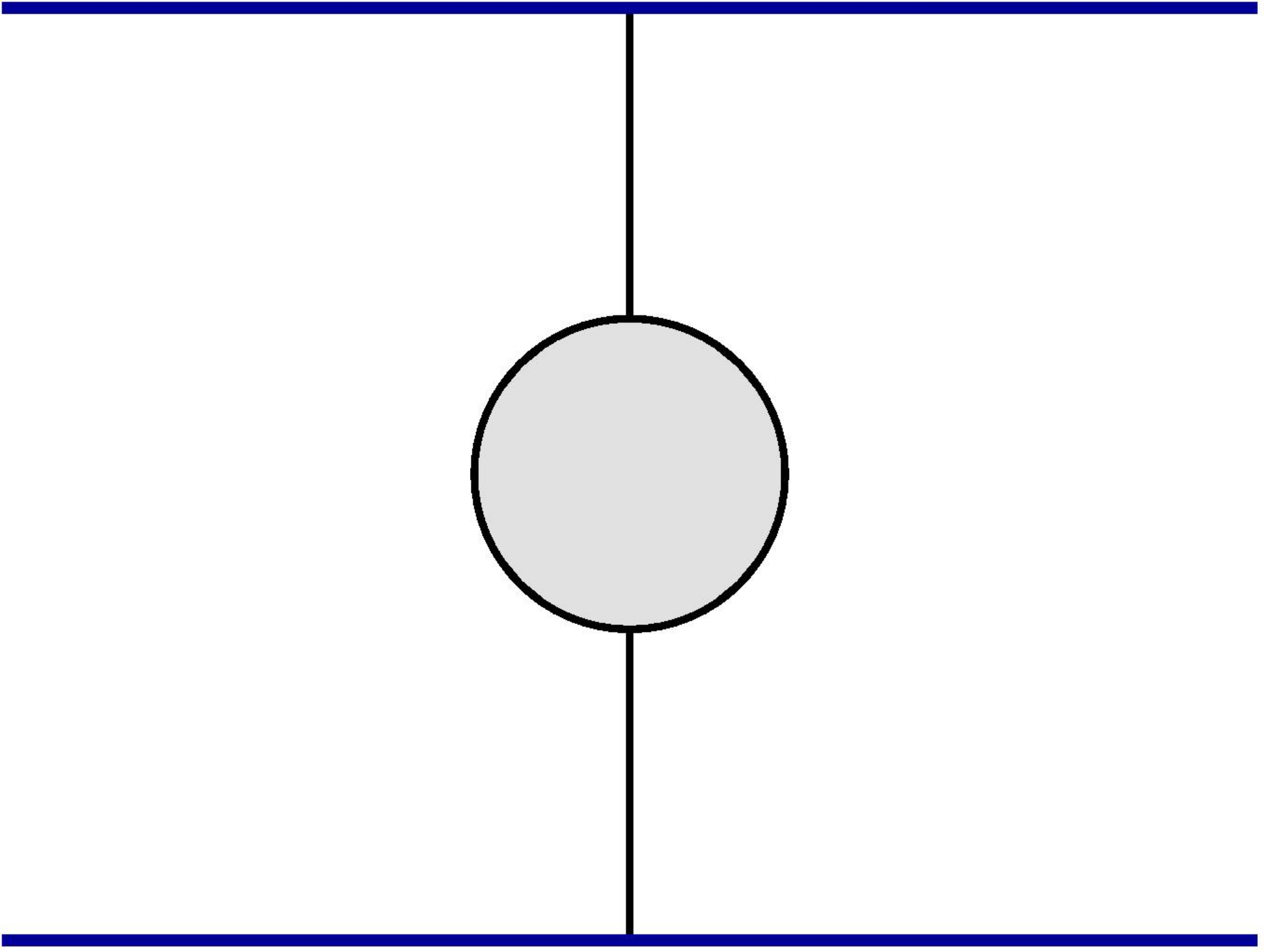
Although the rectangular Wilson loop is not a supersymmetric observable, the diagrams in fig. 3, when combined together, feature spectacular cancellations. In the Feynman gauge the gluon and the scalar propagators are equal. The diagram (a) then renormalizes the effective coupling, and it has been already taken into account by including the $1$ in the definition of $\hat{\lambda}$, eq. (2.6). The sum of the remaining three diagrams can be considerably simplified.

We start with the H-graph, fig. 3(e). The numerator in the corresponding momentum integral (the momentum assignment is shown in fig. 4a), can be written as

$$-(k+q)(2p-k-q)=-2p^{2}+k^{2}+q^{2}+(p-k)^{2}+(p-q)^{2}-(k-q)^{2}.$$

(4.1)

This is the standard Passarino-Veltman reduction. All the terms but one contain a vanishing propagator. Those terms combine into

$$\raisebox{-19.37494pt}{\includegraphics[height=43.05542pt]{Hd.pdf}}=2\left(\partial_{1}+\partial_{2}\right)^{2}\raisebox{-19.37494pt}{\includegraphics[height=43.05542pt]{Hsc.pdf}}+\raisebox{-19.37494pt}{\includegraphics[height=43.05542pt]{Hnw.pdf}}+\raisebox{-19.37494pt}{\includegraphics[height=43.05542pt]{Hsw.pdf}}+\raisebox{-19.37494pt}{\includegraphics[height=43.05542pt]{Hne.pdf}}+\raisebox{-19.37494pt}{\includegraphics[height=43.05542pt]{Hse.pdf}}-\raisebox{-19.37494pt}{\includegraphics[height=43.05542pt]{Xsc.pdf}}$$

(4.2)

The last term exactly cancels with the X-diagram in fig. 3d.

The Y-graph in fig. 3(c) can be reduced to the scalar diagram with the derivatives along the contour, acting on the external lines:

$$\raisebox{-19.37494pt}{\includegraphics[height=43.05542pt]{Ygraph.pdf}}+\raisebox{-19.37494pt}{\includegraphics[height=43.05542pt]{antiYgraph.pdf}}=\raisebox{-19.37494pt}{\includegraphics[height=43.05542pt]{Yw.pdf}}-\raisebox{-19.37494pt}{\includegraphics[height=43.05542pt]{Ye.pdf}}$$

(4.3)

after which the external leg of the diagram can be integrated by parts. The fact that the Y-diagrams gives a total derivative has been observed many times in similar calculations [9, 14]. Upon integration by parts only the boundary terms survive:

$$\raisebox{-19.37494pt}{\includegraphics[height=43.05542pt]{Y1.pdf}}+\raisebox{-19.37494pt}{\includegraphics[height=43.05542pt]{Y2.pdf}}=2\raisebox{-19.37494pt}{\includegraphics[height=43.05542pt]{bubble.pdf}}-\raisebox{-19.37494pt}{\includegraphics[height=43.05542pt]{Y-.pdf}}-\raisebox{-19.37494pt}{\includegraphics[height=43.05542pt]{Y+.pdf}}$$

(4.4)

The last two diagrams cancel off the four middle terms in (4.2). As shown in the appendix A, the bubble diagram cancels with the self-energy corrections in fig 3b. We are thus left with a single contribution, given by the second derivative of the scalar H-graph (fig. 4b):

$$K_{1}(u,v;x)={\hat{\lambda}^{2}}\,\Delta H(x_{1},\ldots,x_{4}),$$

(4.5)

where the Laplacian is defined as

$$\Delta=\left(\partial_{1}+\partial_{2}\right)^{2}.$$

(4.6)

and

$$H(x_{1},x_{2},x_{3},x_{4})={1\over(4\pi^{2})^{5}}\int\;\frac{d^{4}z\;d^{4}y}{(z-x_{1})^{2}\,(z-x_{4})^{2}\,(z-y)^{2}\,(y-x_{2})^{2}\,(y-x_{3})^{2}}$$

(4.7)

The diagram is taken in the following kinematics:

$$x_{1}=(u,0,0,1),~x_{2}=(0,0,0,1),~x_{3}=(x,0,0,0),~x_{4}=(x+v,0,0,0).$$

(4.8)

We do not know if one can express the H-diagrams in terms of known functions. This is a difficult double-triangle two-loop integral, for which we were unable to find any closed analytic expression. The best we could do is a double-integral representation, presented in appendix B. However, for analyzing the strong and weak coupling limits it will suffice to know the asymptotic expressions of the H-diagram, which are relatively easy to get from the Feynman integral directly.

The problem of finding the Coulomb charge at the NLO boils down to solving the linear problem (3.9) with the kernel given by the sum of (3.11) and (4.5). Doing this exactly is rather difficult, as the Schrödinger operator becomes integro-differential, and the eigenvalue $\alpha$ enters the equation non-linearly. However, $\lambda$ is small and we can apply the usual formulas of quantum-mechanical perturbation theory. But as we do not know the leading-order wavefunctions explicitly, we will restrict ourselves to the two limiting cases of small $\hat{\lambda}$ and large $\hat{\lambda}$.

At large $\hat{\lambda}$ the problem significantly simplifies, because then $\alpha$ is large, and the integral transform in (3.9) is highly peaked at small $u$ and $v$, because of the exponential suppression factor. In particular, the scale of variation of the wavefunction is proportional to $\hat{\lambda}^{-1/4}$, cf. (3.15), and is thus much larger than the scale at which the integrand gets exponentially suppressed, which is $\alpha^{-1}\sim\hat{\lambda}^{-1/2}$. We can thus neglect the shift in the argument of $\psi$ by $v-u$ and reduce the problem to the Schrödinger equation with a local effective potential

$$V_{\rm eff}(x)=-\int_{0}^{\infty}du\int_{0}^{\infty}dv\,\,{\rm e}\,^{-\frac{\alpha}{2}\left(u+v\right)}K(u,v;x),$$

(5.1)

Moreover, the kernel itself changes on the distances of order one, and we thus need to know its expansion at small $u$ and $v$. This corresponds to the regime when the end-points of the H-diagram collide pairwise (fig. 1). The relevant limit is computed in eq. (B.8), with logarithmic accuracy:

$$K_{1}(u,v;x)\simeq\frac{\hat{\lambda}^{2}\left(u^{2}\ln u^{2}+v^{2}\ln v^{2}\right)}{256\pi^{6}\left(x^{2}+1\right)^{3}}\,.$$

(5.2)

Substituting this result into (5.1), we get for the effective potential:

$$V_{\rm eff}(x)=-\frac{\hat{\lambda}}{4\pi^{2}\left(x^{2}+1\right)}+\frac{\lambda\hat{\lambda}^{2}\ln\alpha}{2\pi^{6}\alpha^{4}\left(x^{2}+1\right)^{3}}.$$

(5.3)

At strong coupling, when the eigenvalue is given just by the depth of the potential well, we get:

$$\alpha=\frac{\sqrt{\hat{\lambda}}}{\pi}\left(1-\frac{\lambda\ln\hat{\lambda}}{2\hat{\lambda}}\right).$$

(5.4)

The second term in the brackets is the correction to the ladder approximation. Since we have not determined normalization of the logs in (5.2), the answer is calculated with the logarithmic accuracy. It should be possible to more accurately determine all the constants and calculate the non-logarithmic term of order $\lambda/\hat{\lambda}$, but we will not attempt to do it here.

It is a non-trivial fact that the corrected Coulomb charge, as a function of $\lambda$ and $\vartheta$, is still proportional to $\lambda^{1/2}$ and thus can be directly compared to the string calculation at strong coupling. Provided that $\ln\hat{\lambda}$ can be traded for $\vartheta$, in the strong-coupling limit, we get:

$$\alpha=\frac{\sqrt{\lambda}}{2\pi}\,\,{\rm e}\,^{\frac{\vartheta}{2}}\left(1-2\vartheta\,{\rm e}\,^{-\vartheta}\right).$$

(5.5)

The first order of perturbation theory in $\lambda$ for the eigenvalue equation (3.9) produces the following answer for the correction to the Coulomb charge:

$$\delta\alpha={2\lambda\over\alpha_{0}}\,\int\limits_{-\infty}^{\infty}dx\,\int\limits_{0}^{\infty}du\,\int_{0}^{\infty}dv\,\,{\rm e}\,^{-{\alpha_{0}\over 2}(u+v)}\psi_{0}(x)\,\psi_{0}(x-u+v)\,K_{1}(u,v,x),$$

(6.1)

where $K_{1}$ is first correction to the kernel from (4.5)-(4.8). At small $\hat{\lambda}$ the unperturbed wavefunction is given by

$$\psi_{0}(x)\simeq\left(\frac{\alpha_{0}}{2}\right)^{\frac{1}{2}}\,{\rm e}\,^{-\frac{\alpha_{0}}{2}|x|}\,\qquad(\hat{\lambda}\rightarrow 0).$$

(6.2)

Since $\alpha_{0}$, given by eq. (3.13), is parametrically small in $\hat{\lambda}$, all exponential factors in (6.1) decay very slowly and to the first approximation can be set to one, which leads to

$$\delta\alpha=\lambda\hat{\lambda}^{2}\int\limits_{-\infty}^{\infty}dx\,\int\limits_{0}^{\infty}du\,\int_{0}^{\infty}dv\,\Delta H(x_{1},\ldots,x_{4}),$$

(6.3)

where $x_{i}$ are expressed through $u$, $v$ and $x$ according to (4.8), or according to fig. 1. We got the expected result, that to the leading order in $\hat{\lambda}$ it is enough to integrate the H-diagram along the Wilson loop. There are no ladders to sum, as extra rungs of the ladder are accompanied by extra powers of $\hat{\lambda}$. However, as we shall demonstrate in a moment, the integrals in (6.3) actually diverge. To understand how the divergence is cut off, we need to go one step back to the all-loop expression (3.9). The exponential suppression factors in the exact formula becomes important on the scale

$$t_{\rm IR}\sim\alpha_{0}^{-1}\sim\hat{\lambda}^{-1}\,.$$

(6.4)

This scale imposes an effective IR cutoff on the integrals in (6.3).

The integral (6.3) is convergent by power counting, which indicates that nothing special happens when all points go to infinity simultaneously. The divergence comes from the configuration in which $x_{2}$ and $x_{3}$ are a finite distance from one another, while $x_{1}$, $x_{4}$ go to infinity (fig. 5), and from a symmetric configuration in which $x_{1}$, $x_{4}$ stay close, while $x_{2}$, $x_{3}$ go to infinity. In this regime we can use the long-distance approximation (B.9) for the H-diagram. Moreover, we can apply the Laplacian only to the logarithmic prefactor, since the derivatives acting on the other terms in (B.9) raise powers in the denominator, and produce IR convergent integrals. Then, using $\Delta\ln x_{23}^{2}=4/x_{23}^{2}=4/(x^{2}+1)$, we can easily integrate over $x$:

$$\int_{-\infty}^{+\infty}\frac{dx}{x^{2}+1}=\pi.$$

(6.5)

We are thus left with the $u$, $v$ and $z$ integration:

$$\delta\alpha=-2\,\frac{\lambda\hat{\lambda}^{2}}{4^{4}\pi^{7}}\int\limits_{0}^{\infty}du\,\int_{0}^{\infty}dv\,\int\frac{d^{4}z}{z^{2}\left[\mathbf{z}^{2}+\left(u-z^{0}\right)^{2}\right]\left[\mathbf{z}^{2}+\left(v-z^{0}\right)^{2}\right]}\,.$$

(6.6)

The factor of two takes into account the identical contribution from $x_{14}\sim 1$. Doing the $u$ and $v$ integration first, we arrive at

$$\delta\alpha=-\frac{\lambda\hat{\lambda}^{2}}{(2\pi)^{7}}\int\frac{d^{4}z}{z^{2}\mathbf{z}^{2}}\,\left(\frac{\pi}{2}+\arctan\frac{z^{0}}{|\mathbf{z}|}\right)^{2}.$$

(6.7)

The integral is most easily computed by changing variables to $\rho=\sqrt{z^{2}}$ and $\varphi=\arctan(z^{0}/|\mathbf{z}|)$:

$$\delta\alpha=-\frac{\lambda\hat{\lambda}^{2}}{32\pi^{6}}\int^{t_{IR}}\frac{d\rho}{\rho}\,\int_{-\frac{\pi}{2}}^{+\frac{\pi}{2}}\left(\frac{\pi}{2}+\varphi\right)^{2}.$$

(6.8)

The logarithmic divergence at small $\rho$ is fake. It arises because we have initially assumed that $\rho\gg 1$, and neglected, for example, the separation between the two sides of the Wilson loop. The neglected contributions regularize the divergence at some $\rho\sim 1$. On the contrary the IR divergence at large $\rho$ is real, and is regularized only by the resummation of an infinite number of ladder diagrams. The resulting cutoff, up to a numerical factor, is given by (6.4). Taking this relationship into account, we get the final answer for the correction to the Coulomb charge (3.13):

$$\delta\alpha=\frac{1}{96\pi^{3}}\,\lambda\,\hat{\lambda}^{2}\,\log{\hat{\lambda}}$$

(6.9)

Taken at face value, the result (6.9) is a three-loop single-logarithmic correction, which combines with the single-log terms in (3.13). There is also a finite $O(\lambda\hat{\lambda}^{2})$ term, that we have not calculated. Clearly, the higher orders in the ladder expansion will produce single-log contributions of the form $\lambda^{2}\hat{\lambda}\ln\hat{\lambda}$ and $\lambda^{3}\ln\hat{\lambda}$, which originate, for instance, from the purely gluonic H-diagram. It would be interesting to compute these log-enhanced contributions, which complete the perturbative three-loop calculation of the Coulomb charge in the NLLO.

The leading-order ladder resummation can be done also for the Wilson loops on $S^{3}\times R^{1}$ [4]. In $R^{4}$ this configuration maps to a cusp with the opening angle $\varphi$, where $\varphi$ is the angular separation of the Wilson lines on the sphere [15]. Our calculation corresponds to the limiting case $\varphi\rightarrow\pi$. It would be interesting to evaluate the NLO correction for general $\varphi$, especially since the Schrödinger problem is exactly solvable at $\varphi=0$. This latter case corresponds to the straight Wilson line, with the scalar coupling jumping from $0$ to $\cos\theta$ at some point on the contour.

It would be also interesting to reproduce the ladder limit (2.5) from the TBA equations, that in principle describe the Coulomb charge at any value of $\theta$ and $\lambda$ [5, 6]. The TBA equations are highly non-linear, and in general are difficult to solve, but when $\vartheta\rightarrow\infty$ they should reduce to a simple Schrödinger equation (3.12). Such a dramatic simplification is not unconceivable, as $\vartheta$ plays the rôle of a chemical potential in TBA. Large real chemical potential (real $\theta$ actually corresponds to an imaginary chemical potential) should strongly emphasize the degrees of freedom with positive charge, which perhaps can be taken into account by rearranging the ground state of the auxiliary spin system. Whatever the underlying reason for the drastic reduction in complexity in comparison to the general case, in this corner of the parameter space the TBA equations should be solvable.

References

- [1] J. M. Maldacena, “Wilson loops in large N field theories”, Phys. Rev. Lett. 80, 4859 (1998), hep-th/9803002.
- [2] S.-J. Rey and J.-T. Yee, “Macroscopic strings as heavy quarks in large N gauge theory and anti-de Sitter supergravity”, Eur. Phys. J. C22, 379 (2001), hep-th/9803001.
- [3] N. Drukker, D. J. Gross and H. Ooguri, “Wilson loops and minimal surfaces”, Phys. Rev. D60, 125006 (1999), hep-th/9904191.
- [4] D. Correa, J. Henn, J. Maldacena and A. Sever, “The cusp anomalous dimension at three loops and beyond”, JHEP 1205, 098 (2012), 1203.1019.
- [5] N. Drukker, “Integrable Wilson loops”, 1203.1617.
- [6] D. Correa, J. Maldacena and A. Sever, “The quark anti-quark potential and the cusp anomalous dimension from a TBA equation”, 1203.1913.
- [7] J. Erickson, G. Semenoff, R. Szabo and K. Zarembo, “Static potential in N=4 supersymmetric Yang-Mills theory”, Phys.Rev. D61, 105006 (2000), hep-th/9911088.
- [8] E. Shuryak and I. Zahed, “Understanding the Strong Coupling Limit of the Supersymmetric Yang-Mills at Finite Temperature”, hep-th/0308073v2.
- [9] J. K. Erickson, G. W. Semenoff and K. Zarembo, “Wilson loops in N = 4 supersymmetric Yang-Mills theory”, Nucl. Phys. B582, 155 (2000), hep-th/0003055.
- [10] I. R. Klebanov, J. M. Maldacena and C. B. Thorn, “Dynamics of flux tubes in large N gauge theories”, JHEP 0604, 024 (2006), hep-th/0602255.
- [11] T. Appelquist, M. Dine and I. Muzinich, “The Static Limit of Quantum Chromodynamics”, Phys.Rev. D17, 2074 (1978).
- [12] A. Pineda, “The Static potential in N = 4 supersymmetric Yang-Mills at weak coupling”, Phys.Rev. D77, 021701 (2008), 0709.2876.
- [13] N. Drukker and V. Forini, “Generalized quark-antiquark potential at weak and strong coupling”, JHEP 1106, 131 (2011), 1105.5144.
- [14] Y. Makeenko, P. Olesen and G. W. Semenoff, “Cusped SYM Wilson loop at two loops and beyond”, Nucl.Phys. B748, 170 (2006), hep-th/0602100.
- [15] D. Correa, J. Henn, J. Maldacena and A. Sever, “An exact formula for the radiation of a moving quark in N=4 super Yang Mills”, JHEP 1206, 048 (2012), 1202.4455.