On the Nature of $X(4260)$

Assuming that the $X(4260)$ is a $J^{PC}=1^{--}$ chiral singlet particle. The transition operator between photon and $X(4260)$ is as the following:

where we use the anti-symmetric representation $X_{\mu\nu}$ to describe the $1^{--}$ state $X(4260)$, and $F_{\mu\nu}$ denotes the photon field strength. Notice that in the present notation, one has

where we have neglected the electron-positron masses. For $X(4260)$ decay, the following effective lagrangian is used, which is accurate in the leading order in the expansion in terms of $\pi$ momentum in the center of mass frame of $\pi\pi$ system:

where anti-symmetric representation $\psi^{\mu\nu}$ describes $J/\psi$. Up to $O(p^{2}_{\pi})$ level, in Eq. (3) there exist only three independent interaction terms with coefficients $h_{1}$, $h_{2}$ and $h_{3}$. Further, $u_{\mu}=i(u^{+}\partial_{\mu}u-u\partial_{\mu}u^{+})$ and

is the parametrization of the pseudo-goldstone octet:

The chiral symmetry breaking term with coefficient $h_{2}$ in Eq. (3) reads,

Parameters $F_{\pi}$ and $B_{0}$ can be fixed phenomenologically: $F_{\pi}\approx 92.4$MeV and $<0\mid\psi\overline{\psi}\mid 0>=-F^{2}B_{0}[1+O(m_{q})]$. The Eq. (3) can also be rewritten in an explicit form,

We denote the momenta of $e^{-}$, $e^{+}$, $X(4260)$, $J/\psi$, $\pi^{+}$ and $\pi^{-}$ as $q_{1}$, $q_{2}$, $q$, $q_{0}$, $q^{+}$ and $q^{-}$ respectively, see in Fig. 3. The polarization of $J/\psi$ is represented as $\epsilon_{\psi}$, and $k_{\pm}=q^{+}\pm q^{-}$. Then one has the following relations:

where $\rho(s)=\sqrt{1-\frac{4m_{\pi}^{2}}{s}}$.

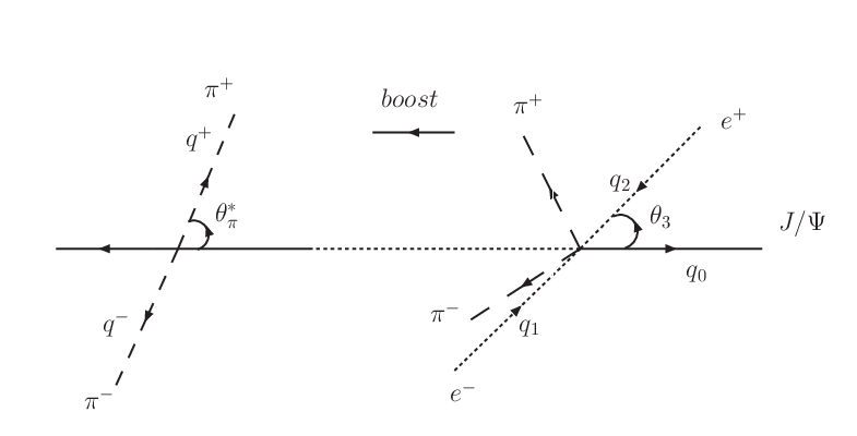
The amplitude of $X\to J/\psi\pi^{+}\pi^{-}$ process at tree level is

where $\alpha,\beta,\lambda$ are Lorentz indices and $D_{X}(q^{2})$ is the denominator of the $X(4260)$ propagator which will be discussed latter.

Following the helicity amplitude decomposition method [36] and choosing the basis of tensors

it is easy to separate the $S$-wave and $D$-wave components of $\pi\pi$ system. The overall $S$-wave amplitude reads,

whereas the $D$-wave part is then

The standard Breit-Wigner type of X(4260) propagator is parametrized as $D_{X}(q^{2})=M^{2}_{X}-q^{2}-iM_{X}\Gamma_{X}(q^{2})$, where $\Gamma_{X}(q^{2})$ is the total decay width including partial width of all possible channels that will be discussed latter.

Since the $D$-wave contribution is proportional to the 4th power of the kinematic factor $\rho(s)$, it is highly suppressed comparing with the $S$-wave contribution. Through numerical studies it is shown that the $D$-wave contribution is roughly less than $1\%$ of the total decay rate, therefore we will not include it in the fitting process in this work.

The tree level amplitude as described in section 2.2 is not sufficient to describe the $X\to J/\psi\pi\pi$ decay process, since the $\pi\pi$ system undergoes strong final state interactions (FSI), especially in $IJ=00$ channel. To include FSI, the following decay amplitude is proposed [37]:

where subscripts 1,2 denote $\pi\pi$ and $K\bar{K}$ final states, respectively. For $A_{2}^{tree}$(the $K\bar{K}$ amplitude), one only needs to change the $m_{\pi}$ into $m_{K}$ in $A_{1}^{tree}$(the $\pi\pi$ amplitude). Especially $T_{11}$, $T_{12}$ and $T_{22}$ represent $\pi\pi\rightarrow\pi\pi$, $\pi\pi\rightarrow K\bar{K}$, $K\bar{K}\rightarrow K\bar{K}$ scattering amplitudes, respectively. Functions $\alpha_{i}$ are mild polynomials which place the role to offset the ‘left hand’ cuts on the complex $s$ plane in amplitude $T$ that would not appear in function $\mathcal{A}$. Expressions in Eq. (13) are remarkable in the sense that the unitarity relations are automatically satisfied. The decay amplitudes $\mathcal{A}_{i}$, as an analytic function of $s$, obey:

In $\alpha_{1}(s)$ an additional pole term is added:

where $s_{A}$ represents the Adler zero of $T_{11}$. The role of the pole term is to cancel the Adler zero hidden in $T_{11}$ but not welcome in $A$ [37]. An advantage of the pole term in Eq. (15) is that, by appropriately choosing coefficient $c^{(1)}_{0}$ as $\lim_{s\to s_{A}}\frac{c^{(1)}_{0}}{s-s_{A}}\,T_{11}(s)=1$, it guarantees

Up to the leading order in $\chi$PT, one finds $c^{(1)}_{0}=16\pi F_{\pi}^{2}$ and $s_{A}=m_{\pi}^{2}/2$ in Isospin 0 S-wave. However in [1,1] Matrix Padé amplitude, $s_{A}=(0.490-0.008i)m_{\pi}^{2}$ and we fix $c_{0}^{(1)}=(0.330-0.001i)\text{GeV}^{2}=(0.779-0.002i)16\pi F_{\pi}^{2}$. ³³ 3 The Adler zero moves to the complex plane because the existence of the left hand cut $(-\infty,4m_{K}^{2}-4m_{\pi}^{2}]$ of $T_{22}$, which has been taken into $T_{11}$ due to Matrix Padé approximation. And so on for that of $c_{0}^{1}$.

In V1, three different representations of $T$ matrices were used for the fit (coupled channel Padé approximation [38], K-matrix unitarization [39] and the PKU representation [40] ), however not much difference was obtained. Therefore we only keep the Padé amplitude in this work to perform the fit to the $\pi\pi$ invariant mass spectrum. In Table 1 we list the low energy constants⁴⁴ 4 We noticed that for these LECs there is a difference between ours [38] ($L_{i}^{O}$) and that in the earlier work [41]($L_{i}^{P}$): $L_{i}^{P}=L_{i}^{O}+\frac{\Gamma_{i}}{32\pi^{2}}$. It is because we calculated in $\overline{MS}$ and theirs in $\overline{MS}-1$. To compare with their work we need to transform our LECs into $L_{i}^{P}$, which has been incorrectly transferred in [38] and we correct it here.). For more details about these T matrices, we refer to the original literature.

Once the $X(4260)\rightarrow J/\psi\pi\pi$ amplitude is calculated from Eq. (13) in above section, one obtains the decay width $\Gamma_{J/\psi\pi\pi}$, the cross section $e^{+}e^{-}\rightarrow X(4260)\rightarrow J/\psi\pi\pi$ and the $\pi\pi$ invariant mass spectrum. In this subsection we focus on how to write down the correct form of denominator of the $X(4260)$ propagator.

Beside the $J/\psi\pi\pi$ channel indicated by the experiment, the X(4260) may also decay into $h_{c}\pi\pi$,and there are other nearby thresholds close to X(4260), such as $\chi_{c0}\,\omega$ (4197MeV), $D_{s}^{*+}\bar{D}_{s}^{*-}$ (4224MeV), $D^{-}D_{1}^{+}(2420)$ (4291MeV), $\chi_{c1}\,\omega$ (4293MeV), etc.. It is possible that X(4260) couples to all these channels. Therefore a careful way is to write down the denominator of the $X(4260)$ propagator as:

where $\Gamma_{X}(q^{2})$ consists of all partial widths,

Here $\Gamma_{J/\psi\pi\pi}(q^{2})$ is calculated from the above amplitude of $X(4260)\rightarrow J/\psi\pi\pi$, and $k_{\omega\chi_{c0}}$, $k_{D_{s}^{*}D_{s}^{*}}$, $k_{DD_{1}}$, $k_{\omega\chi_{c1}}$ are the 3-momentum of $\omega\chi_{c0},D_{s}^{*}D_{s}^{*},DD_{1},\omega\chi_{c1}$ in the $X(4260)$ rest frame, respectively. The $D_{s}^{*}D_{s}^{*}$ channel begins with a P-wave coupling therefore it depends on 3rd-order momentum, and the other three channels are of S-wave couplings and hence only depend on their 1st-order momentum. The possible rest partial widths are parameterized as a constant $\Gamma_{0}$. For $h_{c}\pi\pi$, since the channel momentum $k_{h_{c}\pi\pi}$ behaves like a constant near $q^{2}=M_{X}^{2}$, we parameterize $\Gamma_{h_{c}\pi\pi}$ as a constant, too. Notice that $\Gamma_{h_{c}\pi\pi}/\Gamma_{J/\psi\pi\pi}(M_{X}^{2})$ is constrained by experiment. We discuss this point in more detail in the next section.

One may notice that $Z_{c}\pi$ is also a possible decay channel of the X(4260) but it is not considered in this work, since the contribution of $X(4260)\to Z_{c}\pi\to J/\psi\pi\pi$ can be absorbed into the $XJ/\psi\pi\pi$ contact interaction in the Lagrangian Eq. (3). To confirm this viewpoint, we tested the contribution of $Z_{c}\pi$ with Breit-Wigner parametrization of $Z_{c}$, and found that there was not much difference in $J/\psi\pi\pi$ and $\pi\pi$ spectrums from that without its contribution. Therefore we exclude $Z_{c}\pi$ contribution in this paper and leave it for future work.

In the present work we fit the X(4260) line shape in the region of 4.15GeV$<\sqrt{q^{2}}<4.47$ GeV, where the data is from Ref. [3] (16 data points) and Ref. [5] (16 data points), see in Figure 5a. The total cross section of $e^{+}e^{-}\rightarrow J/\psi\pi\pi$ is given by

where $t=(q-q^{-})^{2}$, $\mathcal{A}_{1}$ is defined in Eq. 13 and the lower and upper limits are given as

With Eq. (20), one finds out that for a larger $q^{2}$, the upper limit of $s$ becomes too large to insure the validity of the parametrization introduced in section 2.3⁵⁵ 5 For $\sqrt{q^{2}}=4.47$GeV, it corresponds to a value $\sqrt{s}\simeq 1.17$GeV which is within the range that $T$ can provide a reasonable description.. For $\pi\pi$ invariant mass spectrum we use the data given in figure 4b of Ref. [3], corresponding to $\sqrt{q^{2}}\in[4.2,4.4]$GeV (17 data points), the data $\sqrt{q^{2}}\in[4.15,4.45]$GeV (41 data points) in Ref. [5], and the data $\sqrt{q^{2}}$ fixed at 4.26GeV(44 points) from the recent experiment [27]. For the first set of data, a MC study of efficiency correction at $\sqrt{q^{2}}=4.26$GeV is given in Ref. [3], and through a numerical test we find that the efficiency curve is well reproduced by the $\pi\pi$ two body phase space up to a normalization constant, hence in our fit we simply use the two body phase space instead of the efficiency corrected one. We assume the other two sets of data maintain similar behavior. Summing up, there are totally 145 data points in $\pi^{+}\pi^{-}$ invariant mass spectrum to be used.

Recently the cross section of $\omega\chi_{c0}$ channel is measured in $[4.21,4.45]$GeV [33, 34], where a rough structure of the $X(4260)$ could be observed at 4.26GeV. If we assume the events in Ref. [33, 34] all come from $X(4260)$ decay, then 9 data points can be used. Nevertheless it may be possible that these events come from continuum rather than from $X(4260)$, hence in our fit we carefully consider this possibility. That is, in the following section 3.2, the fit named Fit I, does not include the $\omega\chi_{c0}$ cross section data, while in section 3.3 the $\omega\chi_{c0}$ cross section data are fitted, named Fit II. It is found that Fit I does not differ much from the result of V1 (notice that here we include the $h_{c}\pi\pi$ channel), but Fit II, with the $\omega\chi_{c0}$ data being included, violates the approximate ‘scaling law’ found in V1 and lead to a small value of $\Gamma_{e^{+}e^{-}}$.

Parameters needed in our fit are the following: Firstly, Eq. (1) and (3) describing the $\gamma$ – $X$ transition and the tree level $X(4260)$ $J/\psi$ $\pi\pi(K\bar{K})$ interactions provide 4 parameters. Secondly, it is found that taking $\alpha_{1,2}(s)$ to be linear polynomials (except the Adler zero term) is already good enough for data fitting, hence the two $\alpha_{i}(s)$ (i=1,2 and each $\alpha_{i}(s)$ contains two parameters) contribute another 4 parameters. Thirdly the mass $M_{X}$ of the $X(4260)$ in the propagator and the coupling constant $g_{\omega\chi_{c0}}$ bring another two parameters. Finally, there are three normalization factors $N_{1}$, $N_{2}$ and $N_{3}$ for the $\pi^{+}\pi^{-}$ invariant mass spectrum of Belle, Babar and BESIII, respectively. After summing up there are totally 13 parameters.

We also studied the parameters $g_{D_{s}^{*}D_{s}^{*}},g_{DD_{1}}$, $g_{\omega\chi_{c1}}$ and $\Gamma_{0}$ through rather extensive numerical tests in different environments, and we found that the $g_{D_{s}^{*}D_{s}^{*}},g_{DD_{1}}$ and $g_{\omega\chi_{c1}}$ are always vanishingly small which suggests that the coupling of X(4260) to $D_{s}^{*}D_{s}^{*}$, $DD_{1}(2420)$ and $\omega\chi_{c1}$ are negligible, compared to $J/\pi\pi$, $\omega\chi_{c0}$ and $h_{c}\pi\pi$. Moreover, the parameter $\Gamma_{0}$ tends to vanish in all different fits and hence it can be ignored too.⁶⁶ 6 It is exactly for this reason we will band the $h_{c}\pi\pi$ width with the $J/\Psi\pi\pi$ width with a ratio $R$ (see Eq. (23)), otherwise the fit program will tend to destroy it. Therefore we will not include the couplings to $D_{s}^{*}D_{s}^{*}$, $DD_{1}(2420)$, $\omega\chi_{c1}$ and $\Gamma_{0}$ in our discussion from now on.

In this fit, named as Fit I, only the $J/\psi\pi\pi$ cross section and $\pi\pi$ invariant mass spectrum are included, but not the $\omega\chi_{c0}$ cross section data which will be analyzed in the next section. About $h_{c}\pi\pi$ channel, however, on one hand, lacking of precision the rough shape is not appropriate to fit [42]. On the other hand, it is not clear yet whether they are from the $X(4260)$ resonance or from the continuous background. Therefore we assume $h_{c}\pi\pi$ has an unknown width in the $X(4260)$ propagator, and it is assumed to be a constant because its threshold is far away from the $X(4260)$ resonance,⁷⁷ 7 In fact, the momentum-dependent width of $h_{c}\pi\pi$ channel with form factor is also tested in the fitting as following, $\displaystyle\Gamma_{h_{c}\pi\pi}(q^{2})\sim\int\frac{\sqrt{(q^{2}-(\sqrt{s}+m_{h_{c}})^{2})(q^{2}-(\sqrt{s}-m_{h_{c}})^{2})}\sqrt{s-4m_{\pi}^{2}}}{4qs}dsd\Omega,$ (21) and $\displaystyle\Gamma_{X}(q^{2})=(\Gamma_{J/\psi\pi\pi}(q^{2})+\Gamma_{h_{c}\pi\pi}(q^{2}))\exp(\frac{q^{2}-M^{2}_{X}}{\Lambda^{2}})+g_{\omega\chi_{c0}}k_{\omega\chi_{c0}}+\cdots.$ This fitting result is always similar with the constant width of $h_{c}\pi\pi$, therefore only the constant $\Gamma_{h_{c}\pi\pi}$ is shown in the text. and it is constrained by the width of $\Gamma_{J/\psi\pi\pi}(q^{2})$ as the following relation

where the coefficient $R=0.66$ is a rough estimation from the ratio of $\sigma_{h_{c}\pi\pi}/\sigma_{J/\psi\pi\pi}$ at $q=4.26$GeV[35]. Of course, we will also test the fits with different $R$ value ranging from 0 to 0.66.

When fit to the $J/\psi\pi\pi$ cross section and the $\pi\pi$ invariant mass, we found that the value of $g_{0}$ has large uncertainty. Since it characterizes the transition between $X(4260)$ and the photon field, or $\Gamma_{X\to e^{+}e^{-}}$ according to Eq. (2), it should not be too large to avoid the upper bound established by an analysis on the BES experiment: Ref. [43] gives $\Gamma_{X\to e^{+}e^{-}}<420$ eV, or most conservatively $<580$ eV, at $90\%$ confidence level. The dependence of $\chi^{2}$ on $g_{0}$ is clearly depicted in Fig. 4 (black square) which exhibits an approximate scaling law on parameter $g_{0}$. When $g_{0}$ increases, parameters $h_{i}$ have to become small to compensate for the experimental value of $\Gamma_{X\to J/\Psi\pi\pi}$ as given in Eq. (3). See Eqs. (1) and (11), it is easy to find out that $\Gamma_{X\to J/\Psi\pi\pi}$ is proportional to the product of $g_{0}$ and $h_{i}$. This mechanism keeps $\Gamma(q^{2})$ of the denominator of $X(4260)$ propagator (see Eq. (17)) almost unchanged when $g_{0}$ varies. As a consequence, $\chi^{2}$ becomes almost inert with respect to the variation of $g_{0}$ when it is large enough since the effect can be counterbalanced by a variation of $h_{i}$. This observation is already made in V1, here we reconfirm the ‘scaling law’ even when $\Gamma_{h_{c}\pi\pi}$ is included.

The ‘scaling law’ means that we can not reliably determine parameter $g_{0}$ at all when $g_{0}$ is large enough. It is important to notice that in Fig. 4 there exists a large enough space for $g_{0}$ to maintain a (almost) minimal $\chi^{2}$, and at lower value it is below the BES $\Gamma_{X\to e^{+}e^{-}}$ bound given in Ref. [43]. As an example, we list the lowest value of $g_{0}$ at 4.24MeV which corresponds to $\Gamma_{X\to e^{+}e^{-}}\simeq 41.1$ eV, and its fitting result is shown in Fig. 5 and Table 2. For this chosen value, Table. 2 indicates the widths of $J/\psi\pi\pi$, $h_{c}\pi\pi$ and $\omega\chi_{c0}$ at $\sqrt{q^{2}}=4.26$ GeV are 32.4 MeV, 21.3 MeV and 49.8 MeV, respectively.

We also search for poles of the $X(4260)$ propagator, and the complex plane is divided into four Riemann sheets by $\Gamma_{J/\psi\pi\pi}$ ($\Gamma_{h_{c}\pi\pi}$) and $\Gamma_{\omega\chi_{c0}}$ defined in Table 3, and the pole positions are presented in Table 4. It is noticeable that there are two pair of poles locating above the $\omega\chi_{c0}$ threshold on the third and fourth sheet, and both of them show around 85 MeV pole width for the X(4260) resonance. According to the pole counting rule in Ref. [44, 45], the two pair of near threshold poles indicate that $X(4260)$ is not like a molecule resonance but more like an ‘elementary’ particle or, in other words, a confining state.

For the purpose in extracting solid physical conclusions, we also varies the coefficient R as $0.56,\,0.46,\,0.36,\,0.26,\,0.16,\,0$ in the fit, and when $R=0$, the fit procedure is very similar with V1[46], where we found a large coupling constant $g_{\omega\chi_{c0}}$ and also the $\chi^{2}$ scaling law on $g_{0}$. It is found that qualitative physical results are not sensitive to the $R$ value, and all the fits with different $R$ maintain the same scaling law on the coupling constant $g_{0}$. In all cases the large coupling of the $\omega\chi_{c0}$ to the X(4260) always exists which coincides with the prediction in V1.

Before going to the next section, a brief conclusion is in order: the fit result shows that the $\chi^{2}$ has an approximate scaling law on $g_{0}$, which could not be determined very well. Two nearby poles are found on the third and fourth Riemann sheet. The fit results are not sensitive to the R value, which indicates that $h_{c}\pi\pi$ only contributes to the X(4260) decay as a smooth background. We predict that the $\omega\chi_{c0}$ channel has a large branching ratio in the X(4260) decay in all cases.

In the above subsection, we confirmed that there should be a sizable contribution from $\omega\chi_{c0}$ channel even when the recent $\omega\chi_{c0}$ cross section data from BESIII collaboration[33, 34] are not taken into consideration. In this subsection, we further include the $\omega\chi_{c0}$ cross section data in our analysis to get a more precise result of $g_{\omega\chi_{c0}}$. This will certainly benefit our understanding on $X(4260)$, provided that those $\omega\chi_{c0}$ data indeed come from $X(4260)$ decay. The cross section of $e^{+}e^{-}\to X(4260)\to\omega\chi_{c0}$ is parameterized as Ref. [4],